Can the Current State Support Mechanisms Help the Growth of Renewable Energies in Wind Markets?

Abstract

The aim of this paper is to provide evidence on the effectiveness of the current state support mechanism incentive adopted by the Italian government in the wind market. In particular, this paper intends to investigate the effectiveness of the auction mechanism as an incentive tool for renewable sources as required by the transposition of Directive 2009/28/EC. In order to demonstrate the economic and financial feasibility of a typical wind-sector investment, we performed a scenario analysis (Monte Carlo simulation) determining a 52,500 Net Present Value (NPV) by varying the key underlying variables of the investment. The results show that with the mechanism currently in place the percentage of positive leveraged NPV is approximately equal to 70%. Despite the state contribution provided through the “Feed-in tariff” mechanism, the profitability of wind projects is not always successful, and this problem could be amplified by the slowness of the authorization procedures. The article offers prime reflections for scholars and policy makers who have long been committed to promoting sustainable development and important considerations on the introduction of further incentive models.

1. Introduction

In recent years, the deterioration of environmental conditions has supported the development of renewable sources [1,2], and several authorities have promoted the adoption of sustainable finance and green policies to stimulate a durable and equal economic growth [3,4,5,6]. For instance, the Energy Union Framework Strategy set out the ambition to move away from an economy dependent on fossil fuels [6] and to reach a 20% share of renewable energy sources out of the gross final energy consumption in 2020, while in 2018 the “Intergovernmental Panel on Climate Change” (IPCC), the main international body for the assessment of climate change, updated a “special report” with the aim of limiting the increase in temperature within 1.5 °C compared to pre-industrial levels [7]. In this context, the responsibility of governments is not only to encourage the ecological transition and to adopt long-term strategies but also to identify the most effective mechanisms to promote them through an efficient allocation of public resources. For this reason, the aim of this article is to investigate whether the current state support mechanism helps the development of renewable energies in wind markets in the most effective way. We decided to investigate the wind sector for two different reasons: on the one hand, because, according to the Italian National Recovery and Resilience Plan (NRRP), the sector in which the greatest investments are expected from both public and private funding are solar and wind, meaning that much of the resources should be directed toward wind projects; on the other hand, because the fifth “Gestore Servizi Energetici” (GSE) call by the Italian Energy Services Operator assigned only 12% of the offer, highlighting that there could be inefficiencies in the current mechanism adopted by the state or problems related to other variables. For this reason, we aim to demonstrate—through a scenario analysis based on the Monte Carlo method—the economic and financial feasibility of a typical wind-sector investment at the prices formed in the auctions, and which remain unchanged for the entire duration of the project. In addition, the choice of the wind-sector is supported by the fact, demonstrated by many studies, that the development of wind energy could provide several benefits and play a crucial role in supporting sustainable development and in limiting the damages to the environment [8,9].

In recent years several academic studies have been dedicated to investment feasibility and the state support mechanism in the renewable energy sector, but no studies on the effectiveness of the current state support mechanism in the wind sector in Italy using a scenario analysis have been found. From a global perspective, different studies have analyzed the role of state incentives in the United States (U.S.) [10,11,12]. Black et al. [10] studied the different types of policies adopted in the western region and demonstrated that financial incentives and renewable portfolio standards can support wind development and the growth of wind energy. Menz and Vachon [11] found a positive relationship between Renewable Portfolio Standard (RPS) policies and wind power development. Horner et al. [12] demonstrate that RPS policies could have significant positive effects on wind innovation, whereas tax-based incentives have not been particularly significant. They also find that public Research and Development (R&D) funding could play a crucial role for wind novation. Sadorsky [13], analyzing 17 countries, among which the U.S., confirms that strong multi-level government supports are necessary to increase the consumption of wind power. As regard India, Sangroya and Nayak [14]—through an econometric analysis—assess and measure the effectiveness of state incentives for the development of wind energy in 26 states. The model shows that the feed-in tariff and captive consumption are significant for wind energy development. Considering the states belonging to the European Union (EU), a relevant and detailed study has been conducted by Gonzalez and Lacal-Arantegui [15]. They not only provide only an overview of the regulatory frameworks across the Member States, but also analyze three main aspects (support schemes, electrical grid issues, potential barriers), considering the goals established for 2020. A detailed research has also been conducted by Kitzing et al. [16]: they investigate and describe the different types of support policies that have been applied in the EU. Monjas-Barroso and Balibrea-Iniesta [17] conducted a comparative study in three countries (Denmark, Finland, and Portugal), evaluating, with real-option methods, an investment project on renewable energy based on wind power. They demonstrate that public support is stronger in Finland, followed by Denmark and Portugal. Kaplan [18] evaluated the current wind energy policies in Turkey, demonstrating that this resource is not efficiently used because of a lack of state incentives which could support the investment. In Italy, Campisi et al. [19] demonstrate that the grid parity in the wind sector is possible only with incentives support. Finally, a significant paper aims to study the role of environmental taxes and regulations on renewable energy generation for developed economies, with data from 1994 to 2018. They show that bureaucratic qualities such as decision-making and trade openness tend to reduce renewable energy generation [20]. In addition to this stream of work, several studies analyze how the development of renewables energies could support tourism and economic growth. In this case, one study investigates the relationship between tourism development, economic growth, renewable energy consumption, and carbon dioxide emissions considering the Organization for Economic Co-operation and Development (OECD) countries [21], and a second one focuses on the relationships between tourism development, renewable energy consumption, and economic growth considering the U.S., France, Spain, China, Italy, Turkey, and Germany [22].

In the first case, the results showed that tourism development has negative and significant effects on CO₂ emissions in Canada, Czechia, and Turkey, while tourism development has positive and significant effects on CO₂ emissions in Italy, Luxembourg, and the Slovak Republic, while the second study provides different specific results for different countries. Along the same line, Isik and Radulesco [23] demonstrate that renewable energy, tourism, capital, and labor force increase economic growth, while Isik et al. [24] show that economic growth, financial development, international trade, and tourism expenditures caused increases in Greece’s CO₂ emissions.

Two other studies [25,26] analyze the case of Pakistan—in the first case, using time series data from 1985 to 2017, they demonstrate that renewable energy has a constructive linkage to Gross Domestic Product (GDP) growth, while the second study determines the asymmetric effect of CO₂ emissions on expenditures, trade, (Foreign Direct Investment) FDI, and renewable energy consumption through an asymmetrical technique (non-linear autoregressive distributed lag).

Another stream of works investigate the validity of the EKC (Environmental Kuznets Curve) hypothesis: Isik et al. [27] test the hypothesis for 10 states, finding that the EKC hypothesis is valid only for Florida, Illinois, Michigan, New York, and Ohio; Isik et al. [28] investigate 50 US states and a Federal District (Washington, DC, U.S.), demonstrating that only 14 states corroborate the hypothesis; Isik et al. [29] investigate OECD countries, demonstrating that the EKC hypothesis is valid for four out of eight countries; Isik et al. [30] analyze the legitimacy of the EKC hypothesis for a group of seven (G7) countries over the period 1995–2015, finding that (i) the tourism-induced EKC hypothesis is valid only for France, (ii) that a rise in renewable energy consumption has a negative (reduction) impact on CO₂ emissions in France, Italy, the UK, and the US, and (iii) that an increase in the receipt of international tourism has a positive impact on Italy’s CO₂ emissions.

A further study which can be included in this group was conducted by Ongan et al. [31], who test the EKC hypothesis decomposing the model and finding that the empirical results of the decomposed and undecomposed models are perfectly opposed to each other.

Additional studies focusing on sustainable development investigate the role on the ecological footprints; for instance, Isik et al. [32] investigate the convergence of the per capita ecological footprint in the U.S., while Alvarado et al. [33] analyze the environmental degradation associated with the ecological footprint in Latin America. Other relevant studies explore (i) the asymmetrical influences of cereal crop production, forestry production, and economic progress on CO₂ emissions in China between 1970 and 2017, through a non-linear Autoregressive Distributed Lag (ARDL) [34], (ii) the links among urban concentration, non-renewable energy use intensity, economic development, and environmental emissions index in China [35], and (iii) the relationship between natural gas consumption and economic growth in Turkey [36].

2. A Comparison between the Different State Support Mechanisms for Wind Plants: Italian vs. European Case

2.1. Italian State Support Mechanism for Wind Plants

The state support mechanism in Italy has undergone several changes over the years. The initial setting, with the Green Certificates, saw a very high level of support aimed at consistently promoting the diffusion of green energy production both through wind farms and through other technologies. The number of plants to produce energy from renewable sources in operation compliant to the Ministerial Decree is equal to 10,028 units (Italian Energy Services Manager (GSE) data (https://www.gse.it/contatore-fer-elettriche, accessed 28 October 2021)), for a total power of about 16 gigawatt (GW), with 4791 wind plants (48%) for a total power of 8.43 GW (51%). These plants benefit from incentives introduced by various laws that have been passed over time:

• N. 456 plants on ex Green Certificate (equal to 6052 megawatt (MW)).
• N. 375 plants on All-Inclusive Tariff (equal to 22 MW).
• N. 1649 plants on Ministerial Decree (M.D.) July 2012 (equal to 1332 MW).
• N. 2268 plants on M.D. June 2016 (equal to 962 MW).
• N. 43 plants on M.D. July 2019 (equal to 52 MW).

On 31 March 2021, the annual wind energy incentivized was equal to almost 16.5 terawatt-hour (TWh), against a cost for the community of €1347 million. Continuing the study, analyzing wind farms with a power greater than 1 MW—which represents 95% of the sample—we found a substantial gap between the measure of the incentive recognized by the legislation that introduced the Green Certificates and a progressive reduction of the community cost for each MW produced, by virtue of the subsequent provisions of the three Ministerial Decrees (M.D.s) that followed one another from 2012 to 2019. Specifically, the annual community cost for each MW produced was significantly reduced, rising from 98.7 €/MW to 10.4 €/MW, with an average value that still remains very high, 81 €/MW, even if destined to a progressive cost saving as the incentives for the older plants end. The contents above are summarized in the table below (

Table 1. Wind plant incentives in Italy.

Wind Plant Incentives	Power Classes [kilowatt (kW)]	Number of Plants [N.]	Power [MW]	Annual Incentive Energy [MW/Year]	Annual Community Cost [€/million (MLN)]	Annual Community Cost [€/MW]
Green Certificates	From 1000 to 5000	47	123	215,811	21
	Above 5000	259	5812	10,620,183	1049
	Subtotal	306	5935	10,835,994	1070	99
M.D. July 2012	From 1000 to 5000	0	0	0	0
	Above 5000	48	1187	2,553,600	140
	Subtotal	48	1187	2,553,600	140	55
M.D. June 2016	From 1000 to 5000	6	23	42,908	3
	Above 5000	38	796	1,763,714	25
	Subtotal	44	819	1,806,622	27	15
M.D. July 2019	From 1000 to 5000	0	0	0	0
	Above 5000	4	46	95,763	1
	Subtotal	4	46	95,763	1	10
	Total	402	7987	15,291,979	1238	81

Source: Own elaboration based on Italian Energy Services Manager (GSE) data.

).

In the last decade, especially because of the excessive community cost of the contributions paid to energy producers, the laws have evolved, with the virtuous purpose of promoting the production of green energy compatible with the reduction of contributions to the minimum necessary amount, by introducing the feed-in tariff and the auction mechanism. In Italy, the company responsible for the subsidies for renewable energy production and energy efficiency (GSE) has the purpose to help achieve a grid parity in the renewable energy sector, by providing a feed-in tariff system [37,38,39]. This system, according to the D.M. of 23 June 2016 and the M.D. of 4 July 2019, offers an incentive mechanism known as “Tariffa Onnicomprensiva”: it is a fixed tariff (€/megawatt-hour (MWh)) applicable to the electricity sold by producers operating in qualified plants powered by renewable sources. According to this approach, the meaning of the “comprehensive” rate is that its value includes an incentive component and a component related to the market price of the electricity fed into the grid. The mechanism that determines the extent of the incentives was designed with the aim of minimizing the amount charged to the community. Indeed, with the auction method, it is assumed that the participants try to win the MW incentivized by offering the highest possible discount percentage, as long as it is compatible with the minimum profitability of their plant. In each auction, a defined number of incentivized megawatts is put up for a tender, which will be assigned until it ends, starting from the participants who have proposed the highest discount compared to the base price established by the legislation and shown in the table below. Therefore, the auctions should make it possible to achieve a double purpose: to contain the community cost and to plan the maximum amount of energy to be incentivized at the national level for each tender (

Table 2. All-inclusive rate for electricity generated by wind farms in Italy, according to the expected regulatory Italian framework of 2019 (annex 1 of draft Decree FER 1—Renewable Energy Sources 1).

Type of Wind Farm	Power (P) (kW)	Tariff (€/MWh)	Useful Life (Years)
Onshore	1 < P ≤ 100	150	20
Onshore	100 < P ≤ 1000	90	20
Onshore	P > 1000	70	20

Source: Italian Energy Services Manager (GSE) data. Note: the table’s values are reduced by 5%, starting from 1 January 2021, for the onshore wind plants.

).

There were three auctions reserved for wind and photovoltaic plants with a power greater than 1 MW, carried out in 2020, in which a total of 1900 MW was put up for tender—500 in the first auction and 700 in each of the following two. The plants awarded in the aforementioned auctions will obviously come into operation in the years following one of the awards (“For the other technologies (hydroelectric, gas, etc.), about 10% of the total MW was made available, cf. art.11 M.D. of 4 July 2019 (IT)”). The purpose of containing the community cost is directly proportional to the extent of the discount offered by the participants. The effectiveness of this mechanism is, however, conditioned by the occurrence of a concrete context of competition between the various operators participating in the auctions. If the plants that have obtained the authorization from the authorities accumulate a power in MW lower than that foreseen for the auction, the competitive context will obviously disappear. In these cases, the participating companies are aware that they will all be beneficiaries of incentivized energy without running the risk of not obtaining the incentive. This circumstance certainly occurred both in Italy and in Germany. In Italy, in none of the auctions carried out in 2020 were all the MW made available awarded. This circumstance led to a lack of competition, as evidenced by the circumstance that we went from a weighted average reduction of the All-Inclusive Tariff for the power of the wind farms of 19.1% in 2019 (year in which all the power available was assigned) to 2.1% in the call of 30.09.2020. In the two subsequent calls, on 31 January 2020 and 29 May 2020, the weighted average discounts were, respectively, 7.6% and 2.7%. The scenario created, in which the authorized projects were made of a total power lower than that available in the auctions, led to the assignment of higher incentives than in the past (with lower reduction percentages), generating a higher community cost, and therefore an extra yield for the energy producer. The lack of planning and control of the development of renewable energy production plants is causing a high social cost for taxpayers and a waste of resources that could be allocated to the development of further projects. As a further confirmation of what has been said, some wind energy producers who were awarded a low incentive rate due to the high discount offered in the 2019 auction, certain that the MW of the next auction (of 2020) would be higher than the demand of the participants, considered it more profitable to renounce the incentive of the 2019 auction, despite having to pay a high penalty for not subscribing to the awarded rate, and participate in the last auction of 2020, winning an incentive rate that was decidedly higher, offering a very low auction discount.

2.2. European State Support Mechanism for Wind Plants

The incentive policy in Italy can be assimilated to that of the main European countries, as they also provide a substantially homogeneous mechanism with a feed-in-premium (floating) assigned through an auction mechanism. The latter guarantees the investor a fixed price for a given time horizon, consisting of an incentive component (floating) and a component related to the market price of the electricity actually fed into the grid. In 2020, seven European countries awarded the successful bidders of wind power plant auctions with incentives of around 8 GW through the auction mechanism. Specifically, they awarded incentives of 7.4 GW for onshore wind power and only 759 MW for offshore wind power. Also in Germany, six of the seven onshore wind auctions held in 2020 were not fully subscribed to because there were not enough authorized projects. In fact, only 2.7 GW of the 3.9 GW offered were awarded (Wind Energy in Europe, 2020 statistics and the outlook for 2021–2025 (https://windeurope.org, accessed 28 October 2021)).The average incentive rate of onshore wind farms assigned in the 2020 auctions of the main European countries is also equal to 59–64 €/MW, as shown in the table below, in line with the Italian weighted average of the first two auctions of the Ministerial Decree of 4 July 2019 (https://www.gse.it/servizi-per-te/fonti-rinnovabili/fer-elettriche/graduatorie, accessed 28 October 2021). The values of the latest auctions in 2020 are not considered, as the discounts are distorted by the anomalous absence of competition between the participants, as shown below (

Table 3. Successful onshore wind auctions and tenders in 2020.

Country	Mw Awarded	Type of Auction	Support Mechanism	Price in €/MWh
France	749.00	Technology-specific	Feed-in premium (floating)	62.9
France	258.00	Technology-specific	Feed-in premium (floating)	59.7
France	520.00	Technology-specific	Feed-in premium (floating)	59.5
Germany	523.00	Technology-specific	Feed-in premium (floating)	57.6–62
Germany	151.00	Technology-specific	Feed-in premium (floating)	57.4–62
Germany	464.00	Technology-specific	Feed-in premium (floating)	59–62
Germany	192.00	Technology-specific	Feed-in premium (floating)	60–62
Germany	285.00	Technology-specific	Feed-in premium (floating)	61.7–62
Germany	659.00	Technology-specific	Feed-in premium (floating)	56–62
Germany	400.00	Technology-specific	Feed-in premium (floating)	55.9–60.7
Greece	153.00	Technology-specific	Feed-in premium (floating)	59.1–69.2
Greece	472.00	Technology-specific	Feed-in premium (floating)	60
Italy	406.00	Technology-specific	Feed-in premium (floating)	56–68.4
Italy	281.00	Technology-specific	Feed-in premium (floating)	66.9–68.5
Italy	259.00	Technology-specific	Feed-in premium (floating)	68.4–68.6
Ireland	479.00	Technology-specific	Feed-in premium (floating)	74

Source: Wind Energy in Europe, 2020 statistics and the outlook for 2021–2025 (https://windeurope.org, accessed 28 October 2021).

).

It must be considered that the profitability of investments, both in Italy and in Europe, does not depend only on the level of incentives, and therefore on the unitary revenue deriving from the sale of energy, but also on other factors. For example, the producibility of the plants is very important. All things being equal, an investment in a wind power plant (as well as in a photovoltaic one) will be the more profitable the more the site where the plant is installed has better characteristics from the point of view of the availability of the natural resource, i.e., if it allows for a greater production of electricity for the same initial investment. To carry out a large-scale comparison, it is therefore necessary to use an average value of the equivalent hours of producibility in European countries. Other factors also contribute to the profitability of investments in wind farms, such as the cost of the significant financial resources necessary to carry them out, as we will analyze later.

3. Methodology

3.1. Variables and Analysis Introduction

The research has been conducted via the use of a Monte Carlo analysis related to a typical investment in the European wind energy production market. This chosen analytical approach is far from accidental. In fact, simulating a sheer number of combinations of the prefixed parameters (see the next paragraph, that introduces the simulation approach), connected to the wind energy investment, helps to glean the pros and cons of this energy initiative, providing not only evidence for the energy producers but also suggestions for more efficient public incentive policies. Indeed, simulating numerous scenarios could be the right way to cover a broad spectrum of possible outcomes corresponding to possible empirical cases. Therefore, by introducing the stochastic variability, it is possible to consider also the variability not directly correlated to the random variable chosen in the simulation setting. This choice is also justified by the presence of several academic studies which use the same methodology in the context of renewable energy [40,41,42].

Methodologically speaking, the scenarios simulated refer to the results of a typical business plan in this specific sector. In other words, the output of the random combination of the variables, drawn randomly (with specific laws, that will be discussed later), is the levered Net Present Value (NPV) of a projection of a structured investment in the wind energy farm, calculated as follows:

$$LeveredNPV=-Equityinitialinvestement+{\displaystyle \sum }_{i=1}^N\frac{FCF{E}_i}{{\left(1+K_e\right)}^i}$$

(1)

where the FCFE (Free Cash Flow to Equity), stands for the residual financial resources available to the shareholders. Meanwhile, the K_e rate is the (expected) percentage cost of Equity capital. The choice of the levered quantity rather than the unlevered one is due to the aim of the research to evaluate the contribution of governments to the development of this production sector and, at the same time, to suggest a more efficient public incentive initiative.

Before proceeding with the analysis, the assumptions regarding the input factors of the business plan considered are presented.

Note that two macro sections of input data have been created for the simulation. The first, named Fixed Data, relates to average data, while the second, named Variable Data, relates to exogen variables.

The classification into two sections (

Table 4. Sections created for the simulation.

1st Section	2nd Section
Fixed Data	Variable Data
Cost of the structure Initial investment Investment structure	Interest rate level Annual energy production hours of the implant Level of the “Feed-in Tariff” (FiT) Cost of equity (Ke)

Source: Own processing.

) was made necessary by the fact that the second group includes the exogenous quantities, that have a greater percentage variability than the others, significantly influencing the economic result and therefore the profitability of the project.

3.1.1. Fixed Data

The next tables indicate the cost structure, the initial investment, with the different cost voices that form this expense, and some other determinants of the specific energy initiative.

The data for the implementation of the simulation, for a typical wind power plant, are provided by Siemens Gamesa Renewable Energy S.A. (a world leader in the renewable energy industry, with more than 35 years of experience in the wind power business, working to provide the world’s offshore and onshore wind turbines and services) through the document provided by Dr. Simone Togni, the president of ANEV (the Italian environmental protection association (recognized pursuant to Law no. 349 of 8 July 1986) founded in July 2002, which brings together about 90 companies operating in the wind sector and over 5000 subjects operating in compliance with its regulations. ANEV is present on the Board of Directors of the corresponding European and World associations, such as WWEA-GWEC-EWEA, a member of UNI-CEI-AIEE. Among the aims of the Association is to contribute to the promotion and use of wind-based energy, as well as to promote research and technological development aimed at the use of wind and the rational use of energy, as well as the dissemination of correct information based on real data) and refer to average market data.

These values (

Table 5. Specific investment.

Cost structure	Value
Initial investment (€)	25,366,600
Useful life (year)	20
Generators (number)	6
Power of each generator (MW)	3.73
Operation and Maintenance (O&M) (€/MW)	15,000
Insurance cost (€/MW)	2300

) are fixed and determine the returns and costs of the project over the years:

As regards the first amount, the initial investment, it is the result of the sum of the cost voices specified in the next table (

Table 6. Initial investment data.

Initial Investment	Value
Connection works (€)	1,911,600
Wind plant (€)	16,020,000
Civil works (€)	3,600,000
Electrical works (€)	3,300,000
Other costs (technical, legal, etc.) (€)	535,000
Total initial cost	25,366,600

Source: Siemens Gamesa Renewable Energy S.A. data.

).

The indicated values are annual costs, except for the initial investment. The generators dimension (3.73 MW) is sufficient to make the wind farm efficient. This parameter, as well as the information on the other costs sketched in the tables, has been obtained by interviewing Europe’s leading producers in this field and validated with some wind farm developers. In what concerns the authority cost, the Italian amount has been assumed (

Table 7. Other financial parameters.

Investment Structure	Value
Inflation growth per year (%)	1.3
Debt/equity (%)	65/35
Tax rate (%)	24
Unlevered Beta	0.68
Levered Beta	1.64
E[rm] (%)	7.11

Source: Own processing based on the European Central Bank database.

), although aligned with the European ones.

The inflation level has been selected to develop a prudential projection of the investment. More specifically, an inflation growth of 1.3% per year has been assumed (the selected value has been deduced based on the inflation growth projection of June 2021, elaborated by the European Central Bank (ECB), https://www.ecb.europa.eu/pub/projections/html/ecb.projections202106_eurosystemstaff~7000543a66.en.html, accessed 28 October 2021). The inflation affects only the cost structure because the energy sale price is fixed in the auction for the investment’s lifetime. In this way, the analysis already considers a more burdensome parameter in order to set a macro prudential analysis. In what concerns the debt–equity ratio, the value shown has been deduced based on several studies concerning the financing structure of this kind of green investments. Angelopoulos et al. [43] have investigated the risk and the cost of capital of this kind of investment in European countries, and they have shown how the ratio largely used by Europe’s leading producers is best approximated by the 65/35 ratio.

The tax rate used in the simulation model takes into consideration the mean corporate tax in the Eurozone. Similar considerations have been applied to the Unlevered Beta (the measure of business risk) of the investment; more precisely, we assumed the value proposed by Stern’s observatory, guided by Aswath Damodaran, for the European green and renewable industry (http://people.stern.nyu.edu/adamodar/New_Home_Page/datacurrent.html, accessed 28 October 2021). The equivalent levered beta has been calculated applying the well-known formula:

$${\beta }_L={\beta }_U\ast \left(1+\frac{D}{E}\ast \left(1-taxrate\right)\right)$$

(2)

The last value in Table 7, E[r_m] (“E” expresses the mathematical expectation of the market return, and this latter element is estimated), the expected market return has been derived from the current value of the European equity market premium (ERP), published by the university data repository just cited. Indeed, it reports a current value for the ERP of 5.56%; using as a proxy of the current risk-free rate the percentage gross return rate of the Italian bond with maturity at 20 years (it has been decided to take the Italian return rate in the Eurozone as reference because, even though Italy is not the state with the lowest country risk, its bonds have a remuneration which is approximately equal to the European mean proxy of the risk-free interest rate), it is possible to infer the expected European market return by the well-known relation, considering the current value of the individuated risk-free rate:

$$ERP+r_f=E\left[r_m\right]$$

(3)

The current value of the gross BTP 20A return rate is 1.55% (a value referred to the last bond auction, on 10 June 2021). Adding this value to the ERP (5.56%), we obtained the value specified in Table 7. Therefore, it can be utilized as a proxy of the expected return in the European market. This value will be very useful in the simulation scheme, for deriving different values of the cost of equity. Indeed, thanks to the derivation of the expected future return of the European market, $K_e$ would be derived by simply moving the future risk-free rate in a modified form of the Capital Asset Pricing Model (CAPM), throwing an overt relation between the chosen risk-free rate and the one which is the component of the cost of debt capital. The logical path will be clear below, where we discuss the aim and the purposes of this deduction. This elaboration is perfectly suitable for the conducted analysis, which is a forward-looking study based on a pure simulation of a future possible value of the levered NPV of a future project.

3.1.2. Variable Data

We decided to simulate a massive amount of scenarios in order to reduce the possible variability derived from the selection of the investment parameters (sketched in the following), which could be reasonably different from the ones chosen in our study. For example, this could be due to different geographical locations of the planned wind energy plant (mostly the geographical volatility of wind intensity), other investment fundamentals, such as the debt-equity ratio, the interest rate level, and the cost of equity, that are quite influent in conditioning the results of the investment.

The Monte Carlo simulation setting, as will be better specified below, is conducted by specifying different probability laws for the economic variables that contribute to determining the outcomes.

The variables identified for the scope, just stated, are:

• The interest rate level.
• The annual energy production hours of the implant.
• The level of the FiT intended as the final energy sale price paid to the energy producers.
• K_e.

These are the cardinal parameters that mainly impact on the result of the investment (levered NPV). The interest rate level principally affects the heaviness of the financing cost structure, like the cost of equity. These would be the real “fly-wheel” in this analysis, because they could be reduced introducing a statal incentive mechanism, and could thus facilitate the access in this specific sector, demolishing entrance barriers that could be quite difficult to overcome for the small and medium-sized firms. The variation of energy production hours has the mentioned aim, since not all the territories have the same fixed exposure to the wind. Therefore, not having indicated any implant site, it has introduced this kind of variation to cover all the possible onshore wind energy projects in Europe. Finally, there is the level of the FiT, which impacts on the definitive price paid to the energy producers and which has been defined after a bearish auction with a given starting point fixed by the energy authority. This variable has been really delicate to manage because of the lack of significant historical data (considering the recent development of this market and the legal and incentive innovation in recent years) (the hypotheses for this variable are discussed below).

The analysis is based on a pure scenario simulation of the possible outcomes of the wind energy investment in the current state of the market, with the aim of revealing an opportunity to enhance the wind energy production market toward a project of statal intervention.

Having described the analysis approach and what it consists of, a wide focus on the above-listed variables is necessary. In what concerns the interest rate level, we assume a variable composed by an index interest rate (EURIRS 20A) plus a supposed interested spread required by the project financing institute, which is normally around 2% (a value obtained by means of interviews to main financial operators and energy sector companies) over the index interest rate.

As was partially anticipated, the algorithm for introducing the variability also in the cost of equity is based on the future variability of the risk-free rate. A modified version of the CAPM classical model has been structured via the aforementioned cited (and now proved) relation between the individuated risk-free rate and the EURIRS 20A. Indeed, thanks to the derivation of the expected future return of the European market, K_e would be derived by simply moving the risk-free rate. More specifically, it has been decided to introduce the financial investment risk (constituted by the cost of the debt capital) in the CAPM model via the risk-free rate, having inferred the historical relation between a given risk-free rate and the market component rate of the interest rate. Therefore, the adjusted CAPM could be represented in this way:

$$E[K_e\left]=E\right[r_f{}^{\ast }]+{\beta }_L\ast \left(\max \left(E\left[r_m-r_f{}^{\ast }\right],E\left[r_d\right]\right)\right)$$

(4)

where $E\left[r_f{}^{\ast }\right]$ is the expected value of the future risk-free rate. Indeed, the forward-looking vision of the analysis requires future projections of the variables in the field, including the future risk-free rate, derived by a fixed effect regression method:

Placing $r_f{}^{\ast }=y$ and $r_d=x$:

$$y_t={\gamma }_0+{\gamma }_1\ast x_t{}^2+\tau +{\epsilon }_t$$

(5)

where τ is the fixed effect variable of the panel data regression. It is assumed that the relation between the two ratios involves other variables, such as the inflation rate in the Eurozone and the remuneration spread among European states bonds. However, these variables are supposed to be fixed in the analysis period considered.

Resorting to the fixed effects transformation:

$$y_t-\ddot{y_t}={\gamma }_1\ast \left(x_t{}^2-\ddot{x_t}\right)+\left({\epsilon }_t-\ddot{{\epsilon }_t}\right)$$

(6)

where:

$$\ddot{y_t}=\frac{{{\displaystyle \sum }}_{t=i}^T{y}_t}{T }; \ddot{x_t}=\frac{{{\displaystyle \sum }}_{t=i}^T{x}_t{}^2}{T }$$

(7)

and so the time-demeaned data:

$$\widehat{y_t}={\gamma }_1\ast \widehat{x_t}+\widehat{{\epsilon }_t}$$

(8)

where the coefficient ${\gamma }_1$ is calculated by means of Pooled OLS.

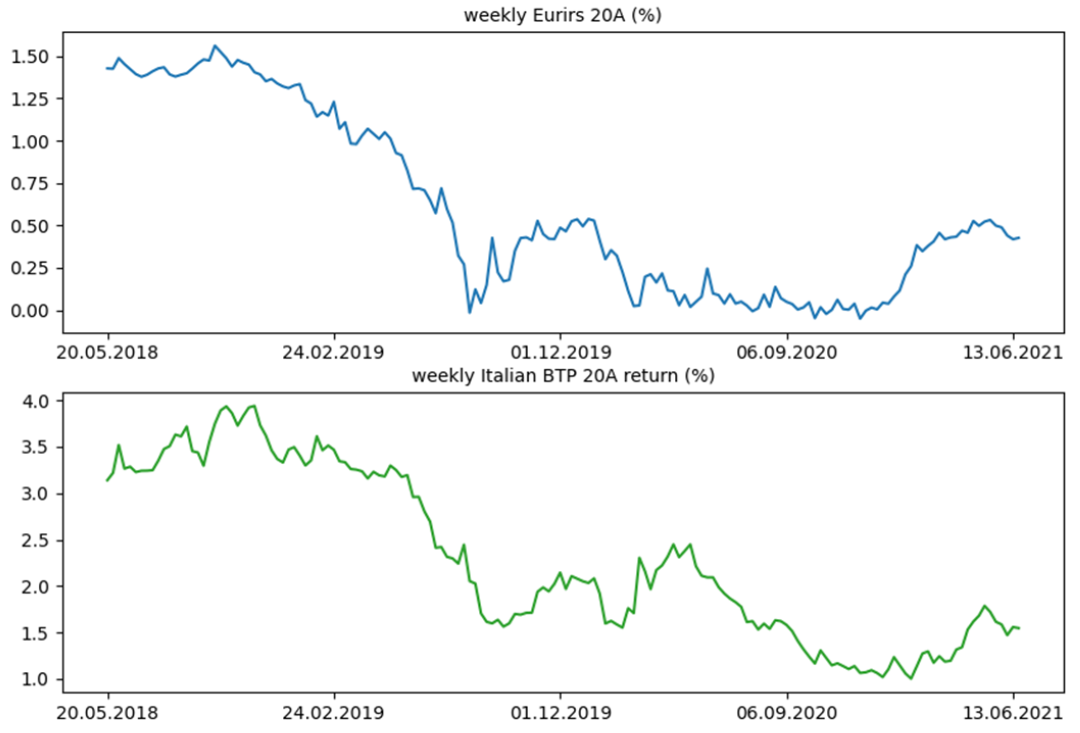
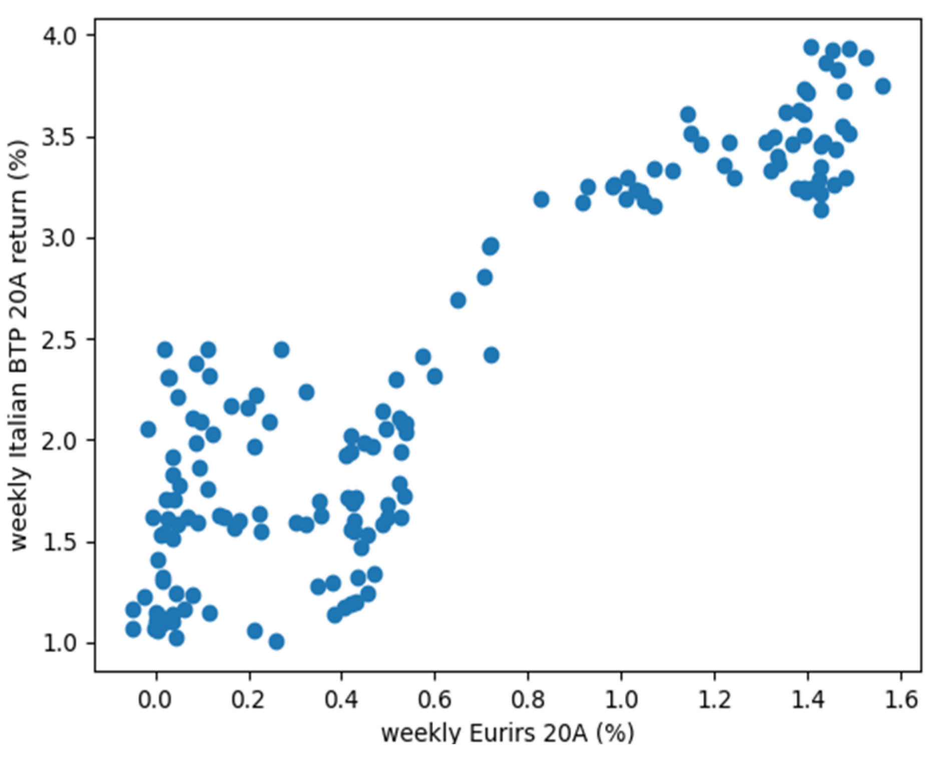
The methodological derivation of $r_f{}^{\ast }$ involves the mentioned historical relation between the two rates specified above. Indeed, in the subsequent section, the linear relation between the referring two rates has been demonstrated. From the scatter plot (Figure 1) of the values or the historical comparison of the two rates (Figure 2), it is evident that the two rates are not linearly related, which is corroborated by the pooled regression analysis summary under the graphs (

Table 8. OLS regression summary statistics.

	Coeff.	Stderr.	t	$\mathit{P}>\left|\mathit{t}\right|$
Const.	3.053 × 10−17	0.0339	9.017 × 10−16	1.000
EURIRSA 20A	0.3759	0.0362	10.381	0.000
R-squared	JB test	Durbin-Watson test
0.8430	2.26	0.193

Source: Own processing based on the European Central Bank database.

).

The Pooled OLS regression has been conducted regressing the weakly EURIRS 20A return collection of data (the dependent variable) on the weekly market component of the $r_d$ (BTP 20A) data. The historical series cover a three-year period, from 17 May 2018 to 6 June 2021.

So, analyzing the summary statistics, it is evident that there is a positive serial correlation of the residuals, albeit these are substantially normally distributed, which is a symptom of the good specification of the model. However, the scope of this introductory analysis is to identify a relation between the two rates specified in order to create a random fluctuation of the cost of equity, linked to the variation of the BTP return rate, toward the CAPM specified above. Therefore, the study of the low positive serial correlation is beyond the scope of this investigation. In the future, it could be investigated in a separate work.

3.2. Into the Simulation Algorithm

As explained in the previous paragraphs, the methodological verification is based on a future investment in the wind energy sector, so it is necessary to consider the time interval needed for completing all the procedures prodrome for the realization of the investment. This sophistication of the analysis is appropriate for both the simulation scheme and the empirical feedback. For this reason, it has been assumed that three months are required for completing all the investment procedures. Most of the efforts have been focused on modeling the distribution of the index interest rate chosen; indeed, a different extraction probability has been considered compared to the uniform one chosen for the other variables, which allowed us to generate values of the variables that are most probably nearer to the current value.

After fixing all the hypothesis, it has been decided to model the interest rate with the model proposed by Cox, Ingersoll, and Ross [44], which is a mean reverting differential equation with a distributed analytical solution (more precisely, the conditional distribution of the interest rate at one year to the current value of the same) as a non-central chi squared variable. Subsequently, the Cox–Ingersoll–Ross model (CIR) on the historical series of the referring interest rate has been fitted in order to estimate the drift and diffusion component of the model. This latter procedure has been conducted via the maximum likelihood method with a starting parameter set obtained with a simple OLS regression, based on the Euler scheme of the stochastic differential equation of the CIR model. Placing $r_d\left(t\right)$ as simply $r\left(t\right)$, and subdividing the three-month period in an arbitrary nuple of time $0=t_1<t_2<\dots \dots <t_n=t$:

$$r\left(t_{i+1}\right)-r\left(t_i\right)=\theta \left(\mu -r\left(t_i\right)\right)\Delta t+\sigma \sqrt{\left|r\left(t_i\right)\right|}\Delta W_i$$

(9)

where μ and σ are the unconditional mean and standard deviation, respectively, of the process. Meanwhile $\Delta W_i$ is the delta of the Wiener process.

Rewriting the aforementioned Euler scheme:

$$\frac{r\left(t_{i+1}\right)-r\left(t_i\right)}{\sqrt{\left|r\left(t_i\right)\right|}}=\frac{\theta \mu }{\sqrt{\left|r\left(t_i\right)\right|}}\Delta t-\theta \sqrt{\left|r\left(t_i\right)\right|}\Delta t+\sigma \Delta W_i$$

(10)

It is evident that this is the structure of a simple linear regression model.

After the estimation of the initial starting parameters, the log likelihood function has been maximized for extracting the most probable parameters of the stochastic model having this specific dataset:

$$lnL\left(\vartheta \right)=\ln p\left(r\left(t_1\right)\right)+{\displaystyle \sum }_{i=1}^{n-1}\ln p(r\left(t_{i+1}\right)|p(\left(r\left(t_i\right)\right),\vartheta )$$

(11)

where $\vartheta =\left(\theta ,\mu ,\sigma \right)$.

This value is easily calculated for the CIR model:

$$lnL\left(\vartheta \right)=\ln p\left(r\left(t_1\right)\right)+\left(n-1\right)\ln c+{\displaystyle \sum }_{i=1}^{n-1}\left\{cr\left(t_i\right)e^{-\theta \Delta t}-cr\left(t_{i+1}\right)+\frac{qcr\left(t_{i+1}\right)}{2cr\left(t_i\right)e^{-\theta \Delta t}}+ln{I}_q\left(2\sqrt{c^{2}r\left(t_i\right)r\left(t_{i+1}\right)e^{-\theta \Delta t}}\right)\right\}$$

(12)

where:

• $c=\frac{2\theta }{{\sigma }^2\left(1-e^{-\theta \Delta t}\right)}$
• $I_q\left(x\right)={\displaystyle \sum }_{i=1}^{+\infty }{\left(\frac{x}{2}\right)}^{2i+q}\frac{1}{i!\Gamma \left(i+q+1\right)}$ is the modified Bessel function of the first kind.

The last step, the numerical maximization of the log likelihood, has been conducted via the gradient descent method. After the estimation of the coefficients of the stochastic equation, the values of the interest rates, conditioned to the value of the current interest rate level, have been extracted according to the non-central chi squared distribution with the parameter estimated:

$$r\left(t_n\right)|r\left(t_1\right)~\frac{1}{2c}{\chi }_d{}^2 with d=\frac{4a\mu }{{\sigma }^2}$$

(13)

and then used as the cost of financing in the simulated cases, both the cost of debt and the cost of equity.

As regards the other variables, the FiT and the production hours are simulated considering a uniform extraction in their prefixed ranges (this probabilistic choice has been guided by the lack of historical data for the FiT variable and by the difficulty in individuating the distribution of the wind energy production hours, due to the aforementioned analytical choice of not considering any specific geographical site in Europe):

• For production hours: [1900, 2300] with a step of 5.33.
• For the FiT case: step of 0.08 [59, 64].

The other aspect that deserves an ad hoc specification is the relation among the variables. Indeed, the independence among variables was assumed. This feature is perfectly logical, since the variables belong to different phenomena, which are not correlated or very poorly correlated (as the case of the interest rate variable and the price of the energy, which could be poorly related to each other (it has been chosen not to consider this relation in the analysis, because it was retained that the effect of the change in the price of energy on the cost of financing would be negligible, which is due to the slowness of the energy sale price’s adaptation to the rapidly and continuous change of rates)).

Regarding the number of scenarios simulated, even if it would seem insufficient to cover all the possible random combinations, the simulation of a sufficiently large volume of scenarios produces approximately the same proportion between a positive NPV and the total number of cases simulated, exploiting considerations based on the law of large numbers. Indeed, considering the number of the negative NPV specified as a random variable linked to the number of simulations “n” represented as a sum of indicator functions linked to the condition of NPV < 0:

$${\displaystyle \sum }_{i=1}^n{1}_{\left(NPV<0\right)}$$

(14)

with:

$$1_{\left(NPV<0\right)}=\{\begin{array}{c}1 ifNPV<0\\ 0 ifNPV>0\end{array}$$

(15)

If we consider the sample mean of this variable, taking the limit of “n” to infinity, the sample mean will converge in probability to the real value of the mean, which is the theoretical population proportion of the negative NPV. In light of this, by stressing the number of simulations (“n”), it is possible to reach a good approximation of the real proportion. These deductions are due to the well-known convergence in probability of the sample mean to the population mean, which is a consequence of the (weak) law of large numbers [45]:

$$P\left(\underset{n\to \infty }{\lim }\frac{1}{n}{\displaystyle \sum }_{i=1}^n{1}_{\left(NPV<0\right)}=Populationproportion\right)=1$$

(16)

4. Results and Discussion

The results obtained, simulating 52,500 scenarios, are unpredictable. In the present condition of the market, the approximated (sampling) percentage of the negative NPV is 30.047%. In Figure 3, below, the dispersion of the random combinations is shown in a 3D plot.

The analysis of the variables that influence the profitability of wind projects in the current Italian economic and regulatory context (comparable to other European countries), has allowed us, firstly, to produce considerations on the impacts of production costs and, secondly, on the additional costs related to the variability of market conditions. In particular, the results show that by simulating a considerable number of scenarios, with the mechanism currently in place, the percentage of positive leveraged NPV is approximately equal to 70%. In addition, to evaluate the positive NPVs, these data also provide a good proxy for assessing business risk in the wind sector in Europe.

However, the aim of this research was precisely to verify whether the current state support mechanisms can incentivize, or continue to incentivize, the growth of renewable energy in the wind market, considering their strategic importance in the context of the new Next Generation EU plan adopted by the European Commission.

The answer is doubtful and could be due to double evidence. Firstly, our study leads to a positive NPV of 70%, meaning that there is still a certain high margin to be filled to guarantee a safe economic return. Furthermore, this work did not consider or model other variables that influence entrepreneurial risk, such as:

• The authorization process for plants powered by renewable energy, which at present appears to be very slow.
• The risk associated with the challenge activities of environmentalist committees for the protection of the landscape and habitat.

Both variables, although profoundly different, could slow down or block the entrepreneurial process in Italy, where the last two auctions of the GSE (4^th and 5^th call of 2021) have been almost deserted, assigning, respectively, 25% and 12% of the offer.

5. Conclusions and Implications

This research investigates the variables that express the economic feasibility of building wind farms using the state incentive rate. The results are not encouraging because, despite the state contribution provided through the FiT mechanism, the profitability of wind projects is not always successful and includes margins of uncertainty amplified by the slowness of the authorization procedures and by the risk associated with the activities of the environmental committees for the protection of the landscape and habitat. In light of these results, a standardization of the administrative process is necessary in the countries belonging to the European Union, and further mechanisms such as the state guarantee should be implemented to mitigate the cost for the company given by the differential between the market price and the price guaranteed by the state (i.e., the price of auction).

This research opens new lines of research aimed at investigating whether, with the presence of a public guarantee, the proxy of the business risk could rise up to 100% of the cases. Indeed, with the presence of a public guarantee, the investment could benefit from the combined effect of both the reduction in the cost of capital and the reduction of indebtedness, which allows the investment to be profitable for two different reasons: the lower perceived risk and a lower and guaranteed energy price throughout the investment period (usually 20 years). It is worth remembering that Member States must collectively guarantee a share of energy from renewable sources of at least 32% in 2030. Therefore, the adoption of more efficient systems in the sector could bring a significant increase in the promotion and development of renewable energy with the same number of resources.

References

1. Sahu, B.K. A study on global solar PV energy developments and policies with special focus on the top ten solar PV power producing countries. Renew. Sustain. Energy Rev. 2015, 43, 621–634. [Google Scholar] [CrossRef]
2. Zhou, N.; Liu, N.; Zhang, J.; Lei, J. Multi-Objective Optimal Sizing for Battery Storage of PV-Based Microgrid with Demand Response. Energies 2016, 9, 591. [Google Scholar] [CrossRef]
3. European Commission. Climate Action Paris Agreement. 2015. Available online: https://ec.europa.eu/clima/policies/international/negotiations/paris_en (accessed on 28 October 2021).
4. European Commission. Action Plan: Financing Sustainable Growth. 2018. Available online: https://ec.europa.eu/info/publications/sustainable-finance-renewed-strategy_en (accessed on 28 October 2021).
5. United Nations. Transforming our world: The 2030 Agenda for Sustainable Development. 2015. Available online: https://sdgs.un.org/2030agenda (accessed on 28 October 2021).
6. European Commission. Fourth Report on the State of the Energy Union. 2019. Available online: https://ec.europa.eu/info/publications/4th-state-energy-union_en (accessed on 28 October 2021).
7. IPCC. Global Warming of 1.5 °C. 2018. Available online: https://www.ipcc.ch/sr15/ (accessed on 28 October 2021).
8. Xu, Z.; Qian, K. Study on the Importance of Wind Energy Development. Appl. Mech. Mater. 2012, 268–270, 958–961. [Google Scholar] [CrossRef]
9. Nix, G. Wind Energy as a Significant Source of Electricity. In Proceedings of the Conference 18th World Energy Engineering Conference, Atlanta, GA, USA, 8–10 November 1995. [Google Scholar]
10. Black, G.; Holley, D.; Solan, D.; Bergloff, M. Fiscal and economic impacts of state incentives for wind energy development in the Western United States. Renew. Sustain. Energy Rev. 2014, 34, 136–144. [Google Scholar] [CrossRef]
11. Menz, F.; Vachon, S. The effectiveness of different policy regimes for promoting wind power: Experiences from the states. Energy Policy 2006, 34, 1786–1796. [Google Scholar] [CrossRef]
12. Horner, N.; Azevedo, I.; Hounshell, D. Effects of government incentives on wind innovation in the United States. Environ. Res. Lett. 2013, 8, 044032. [Google Scholar] [CrossRef] [Green Version]
13. Sadorsky, P. Wind energy for sustainable development: Driving factors and future outlook. J. Clean. Prod. 2021, 289, 125779. [Google Scholar] [CrossRef]
14. Sangroya, D.; Nayak, J. Effectiveness of state incentives for promoting wind energy: A panel data examination. Front. Energy 2015, 9, 247–258. [Google Scholar] [CrossRef]
15. Serrano Gonzalez, J.; Lacal-Arantegui, R. A review of regulatory framework for wind energy in European Union countries: Current state and expected developments. Renew. Sustain. Energy Rev. 2016, 56, 588–602. [Google Scholar] [CrossRef]
16. Kitzing, L.; Mitchell, C.; Morthorst, P.E. Renewable energy policies in Europe: Converging or diverging? Energy Policy 2012, 51, 192–201. [Google Scholar] [CrossRef] [Green Version]
17. Monjas-Barroso, M.; Balibrea-Iniesta, J. Valuation of Projects for Power Generation with Renewable Energy: A Comparative Study Based on Real Regulatory Options. Energy Policy 2013, 55, 335–352. [Google Scholar] [CrossRef]
18. Kaplan, Y.A. Overview of wind energy in the world and assessment of current wind energy policies in Turkey. Renew. Sustain. Energy Rev. 2015, 43, 562–568. [Google Scholar] [CrossRef]
19. Campisi, D.; Gitto, S.; Morea, D. Effectiveness of incentives for wind energy: Models and empirical evidences from an Italian case study. J. Sustain. Sci. Manag. 2016, 11, 39–48. [Google Scholar]
20. Shahzad, U.; Radulescu, M.; Rahim, S.; Isik, C.; Yousaf, Z.; Ionescu, S.A. Do Environment-Related Policy Instruments and Technologies Facilitate Renewable Energy Generation? Exploring the Contextual Evidence from Developed Economies. Energies 2021, 14, 690. [Google Scholar] [CrossRef]
21. Dogru, T.; Bulut, U.; Kocak, E.; Isik, C.; Suess, C.; Sirakaya-Turk, E. The nexus between tourism, economic growth, renewable energy consumption, and carbon dioxide emissions: Contemporary evidence from OECD countries. Environ. Sci. Pollut Res. 2020, 27, 40930–40948. [Google Scholar] [CrossRef] [PubMed]
22. Isik, C.; Dogru, T.; Turk, E.S. A nexus of linear and non-linear relationships between tourism demand, renewable energy consumption, and economic growth: Theory and evidence. Int. J. Tour. Res. 2017, 20, 38–49. [Google Scholar] [CrossRef]
23. Isik, C.; Radulescu, M. Investigation of the relationship between renewable energy, tourism receipts and economic growth in Europe. Stat.-Stat. Econ. J. 2017, 97, 85–94. [Google Scholar]
24. Işik, C.; Kasımatı, E.; Ongan, S. Analyzing the causalities between economic growth, financial development, international trade, tourism expenditure and/on the CO2 emissions in Greece. Energy Sources Part B Econ. Plan. Policy 2017, 12, 665–673. [Google Scholar] [CrossRef]
25. Rehman, A.; Ma, H.; Ahmad, M.; Ozturk, I.; Işık, C. Estimating the connection of information technology, foreign direct investment, trade, renewable energy and economic progress in Pakistan: Evidence from ARDL approach and cointegrating regression analysis. Environ. Sci. Pollut. Res. 2021, 28, 50623–50635. [Google Scholar] [CrossRef] [PubMed]
26. Rehman, A.; Ma, H.; Ahmad, M.; Ozturk, I.; Işık, C. An asymmetrical analysis to explore the dynamic impacts of CO2 emission to renewable energy, expenditures, foreign direct investment, and trade in Pakistan. Environ. Sci. Pollut. Res. 2021, 28, 53520–53532. [Google Scholar] [CrossRef]
27. Işık, C.; Ongan, S.; Özdemir, D. Testing the EKC hypothesis for ten US states: An application of heterogeneous panel estimation method. Environ. Sci. Pollut. Res. 2019, 26, 10846–10853. [Google Scholar] [CrossRef]
28. Isik, C.; Ongan, S.; Özdemir, D. The economic growth/development and environmental degradation: Evidence from the US state-level EKC hypothesis. Environ. Sci. Pollut. Res. 2019, 26, 30772–30781. [Google Scholar] [CrossRef]
29. Isik, C.; Ongan, S.; Ozdemir, D.; Ahmad, M.; Irfan, M.; Alvarado, R.; Ongan, A. The increases and decreases of the environment Kuznets curve (EKC) for 8 OECD countries. Environ. Sci. Pollut. Res. 2021, 28, 28535–28543. [Google Scholar] [CrossRef] [PubMed]
30. Ișik, C.; Ahmad, M.; Pata, U.K.; Ongan, S.; Radulescu, M.; Adedoyin, F.F.; Bayraktaroğlu, E.; Aydın, S.; Ongan, A. An Evaluation of the Tourism-Induced Environmental Kuznets Curve (T-EKC) Hypothesis: Evidence from G7 Countries. Sustainability 2020, 12, 9150. [Google Scholar] [CrossRef]
31. Ongan, S.; Isik, C.; Ozdemir, D. Economic growth and environmental degradation: Evidence from the US case environmental Kuznets curve hypothesis with application of decomposition. J. Environ. Econ. Policy 2021, 10, 14–21. [Google Scholar] [CrossRef]
32. Işık, C.; Ahmad, M.; Ongan, S.; Ozdemir, D.; Irfan, M.; Alvarado, R. Convergence analysis of the ecological footprint: Theory and empirical evidence from the USMCA countries. Environ. Sci. Pollut. Res. 2021, 28, 32648–32659. [Google Scholar] [CrossRef]
33. Alvarado, R.; Tillaguango, B.; Dagar, V.; Ahmad, M.; Işık, C.; Méndez, P.; Toledo, E. Ecological footprint, economic complexity and natural resources rents in Latin America: Empirical evidence using quantile regressions. J. Clean. Prod. 2021, 318, 128585. [Google Scholar] [CrossRef]
34. Rehman, A.; Ulucak, R.; Murshed, M.; Ma, H.; Işık, C. Carbonization and atmospheric pollution in China: The asymmetric impacts of forests, livestock production, and economic progress on CO2 emissions. J. Environ. Manag. 2021, 294, 113059. [Google Scholar] [CrossRef] [PubMed]
35. Ahmad, M.; Işık, C.; Jabeen, G.; Ali, T.; Ozturk, I.; Atchike, D.W. Heterogeneous links among urban concentration, non-renewable energy use intensity, economic development, and environmental emissions across regional development levels. Sci. Total Environ. 2021, 765, 144527. [Google Scholar] [CrossRef]
36. Işik, C. Natural gas consumption and economic growth in Turkey: A bound test approach. Energy Syst. 2010, 1, 441–456. [Google Scholar] [CrossRef]
37. GSE. Accesso Agli Incentivi. Available online: https://www.gse.it/servizi-per-te/fonti-rinnovabili/fer-elettriche/incentivi-dm-06-07-2012 (accessed on 28 October 2021).
38. GSE. Conto Energia. Available online: https://www.gse.it/servizi-per-te/fotovoltaico/conto-energia (accessed on 28 October 2021).
39. GSE. Studi e Scenari. Available online: https://www.gse.it/dati-e-scenari/studi-e-scenari (accessed on 28 October 2021).
40. Chen, T.; Yu, O.; Hsu, G.; Hsu, F.; Sung, W. Renewable energy technology portfolio planning with scenario analysis: A case study for Taiwan. Energy Policy 2009, 37, 2900–2906. [Google Scholar] [CrossRef]
41. Di Leo, S.; Pietrapertosa, F.; Salvia, M.; Cosmi, C. Contribution of the Basilicata region to decarbonisation of the energy system: Results of a scenario analysis. Renew. Sustain. Energy Rev. 2021, 138, 110544. [Google Scholar] [CrossRef]
42. Spiecker, S.; Weber, C. The future of the European electricity system and the impact of fluctuating renewable energy—A scenario analysis. Energy Policy 2014, 65, 185–197. [Google Scholar] [CrossRef]
43. Angelopoulos, D.; Brückmann, R.; Jirouš, F.; Konstantinavičiūtė, I.; Noothout, P.; Psarras, J.; Tesnière, L.; Breitschopf, B. Risks and cost of capital for onshore wind energy investments in EU countries. Energy Environ. 2016, 27, 82–104. [Google Scholar] [CrossRef] [Green Version]
44. Cox, J.C.; Ingersoll, J.E.; Ross, S.A. A Theory of the Term Structure of Interest Rates. Econometrica 1985, 53, 385–407. [Google Scholar] [CrossRef]
45. Jacod, J.; Protter, J.J.P. Probability Essentials; Springer: Berlin, Germany, 2004. [Google Scholar] [CrossRef]
Figure 1. Historical comparison. Source: Own processing based on the European Central Bank database.
Sustainability 13 12094 g001
Figure 2. Scatter plot. Source: Own processing based on the European Central Bank database.
Sustainability 13 12094 g002
Figure 3. Simulation. Source: Own processing.
Sustainability 13 12094 g003