Abstract
In this study, based on the multi-source nature and humanities data of 270 Chinese cities from 2007 to2018, the spatio-temporal evolution characteristics of SO2 emissions are revealed by using Moran’s I, a hot spot analysis, kernel density, and standard deviation ellipse models. The spatial scale heterogeneity of influencing factors is explored by using the multiscale geographically weighted regression model to make the regression results more accurate and reliable. The results show that (1) SO2 emissions showed spatial clustering characteristics during the study period, decreased by 85.12% through pollution governance, and exhibited spatial heterogeneity of differentiation. (2) The spatial distribution direction of SO2 emissions’ standard deviation ellipse in cities was “northeast–southwest”. The gravity center of the SO2 emissions shifted to the northeast, from Zhumadian City to Zhoukou City in Henan Province. The results of hot spots showed a polarization trend of “clustering hot spots in the north and dispersing cold spots in the south”. (3) The MGWR model is more accurate than the OLS and classical GWR regressions. The different spatial bandwidths have a different effect on the identification of influencing factors. There were several main influencing factors on urban SO2 emissions: the regional innovation and entrepreneurship level, government intervention, and urban precipitation; important factors: population intensity, financial development, and foreign direct investment; secondary factors: industrial structure upgrading and road construction. Based on the above conclusions, this paper explores the spatial heterogeneity of urban SO2 emissions and their influencing factors, and provides empirical evidence and reference for the precise management of SO2 emission reduction in “one city, one policy”.
1. Introduction
As people’s living quality has improved, their pursuit of extravagant material enjoyment has escalated, leading to environmental destruction and pollution. The main type of environmental pollution in China is industrial pollution, and these pollutants are divided into three states: stationary, liquid, and gaseous. Among them, the impact of gaseous pollution on the public is particularly obvious [1,2,3]. In the winter of 2013, severe haze events impacted many parts of China on a large scale. Since then, air pollution has gradually aroused widespread concern in society. Since the reform and opening up, the rough industrialization development pattern has played an effective role in promoting the development of China’s economy. However, as a consequence of excessive resource consumption, China is gradually becoming one of the most polluted countries in the world. In particular, SO2 has become one of the major pollutants of PM2.5 and acid rain [4]. As the “invisible killer” of the “smog incident” in London, England, in 1952, SO2 has been classified as a Class III carcinogen by the World Health Organization. SO2 can seriously damage the health of the public, even killing people due to chest congestion, suffocation, cancer, and traffic accidents [5]. According to the 2018 Global Environmental Performance Index report jointly released by Yale University and Columbia University, China ranked 177th in the world, just ahead of India, Bangladesh and Nepal. In China, as one of the world’s largest developing countries, air pollution cannot be ignored.
Fortunately, the rapidly growing SO2 emissions have attracted extensive attention from all sectors of society. Since China joined the East Asia Acid Deposition Monitoring Network in 1998, increasing attention has been paid to the monitoring of SO2 emissions and concentrations in the atmosphere. In 2002, the monitoring stations at all levels of China’s Environmental Protection Administration (now known as the Ministry of Natural Resources) carried out a general survey of acid rain. In 2007, China’s 11th Five-Year Plan linked the environmental protection assessment to the promotion of government officials for the first time. At the same time, a series of important documents, such as the assessment measures for the total emission reduction in major pollutants (GF(2007) No. 36), were issued. In 2012, the Ministry of Environmental Protection (now the Ministry of Natural Resources) formulated and issued a scheme for setting up the national ambient air monitoring network (cities above prefecture level) in the 12th Five-Year Plan (HF(2012) No. 42). Among the national ambient air quality monitoring networks at the national, provincial, municipal, and county levels, SO2 ranked first in the detection projects of urban air, background air, regional air, and acid rain, which shows that SO2 is one of the representative pollutants used for evaluating the regional ambient air quality, and that it affects the regional transmission mechanisms of pollutants.
The report of the 19th National Congress of 2017 forwarded the battle of pollution prevention and control, and Premier Li Keqiang also emphasized that the emission of sulfur dioxide, nitrogen oxides, and PM2.5 should be controlled to ensure the “victory of the blue sky defense war” in the same year’s “Government Work Report”. Therefore, determining the main influencing factors of urban SO2 emissions has become an urgent task, and this is also a prerequisite for subsequent industrial policy decision making and management optimization.
At present, the research on air pollution mainly focuses on AQI, PM2.5, PM10, CO, NO2, SO2, and other major pollutants [6,7]. There are a considerable amount of studies on the causes [8], hazards [9], spatio-temporal evolution [10], influencing factors [11], and governance models of air pollution [12]. The influencing factors of air pollution are a comprehensive result of natural and human factors [13]. Natural factors include rainfall, temperature, climate, wind, and terrain, while anthropic factors include the economy, industry, population, technology, policy, culture, and trade. The research data were mainly obtained from statistical yearbooks, satellite remote sensing data inversion, monitoring stations, news media reports, etc. [14]. The evolution of air pollution can be explored based on big data from different time dimensions, such as hourly, weekly, quarterly, and annual perspectives [15].
Some researchers have discussed the impact mechanisms of the COVID-19 pandemic [16], urbanization [17], foreign direct investment [18], climate change [19], carbon emissions trading [20], meteorological conditions [21], and tourism development [22] on air pollution. The results of this research have shown a negative inhibition, positive promotion, or nonlinear effects. In addition, the direct and indirect external influences of urban air pollution on socio-economic development, anthropic activities, and natural ecosystems have also been discussed. For instance, some researchers have also discussed the external effects of urban air pollution on families’ economic costs [23], residents’ health levels [24], urban crime rates [25], and electricity consumption [26]. Therefore, there may be endogenous causal relationships between air pollution and relevant variables. The same influencing factors may have uncertain effects on SO2 emissions with multiscale spatial synergy or trade-offs, which results in significant spatial heterogeneity effects. It is necessary to select a suitable research model to effectively identify the robust influencing factors.
In terms of research methods, there are many models used to study the causes of air pollution, such as the Bayesian [27] and spatial econometric models [28], the generalized divisia index approach [29], geographic probes [8], and GWR [30]. Liu et al. used the MGTWR model to infer PM 2.5 at non-sampled points, and applied the posterior uncertainty assessment value to improve the model’s accuracy [31]. The reason for this is that the spatial econometric model can avoid spatial autocorrelation and spillover effects compared with the general model, and its regression results are more robust. At the same time, spatial econometric models generally require a large number of microscopic data samples, especially the scale selection of regional research samples. As spatial data, information about regional SO2 emissions includes a series of location attributes and may cause spatial effects, such as spatial dependence and spatial heterogeneity, which violate the basic assumptions of OLS and cause estimate bias.
The size of the study region’s scale determines the reference value of its findings. Large-scale studies provide the framework for regional strategies, medium-scale studies lay the basis for regional planning and cooperation, and small-scale studies determine specific regional responses. The study areas for air pollution research include provinces, cities [32], urban agglomerations, and typical areas of watersheds [28], mainly including Beijing, Shanghai, Guangzhou, Beijing–Tianjin–Hebei, Yellow River Basin, and Yangtze River Basin. It can be seen that the smaller the scale of a regional study, the more precise and specific the regional policy regime will be. Therefore, we use a study sample of 270 cities in China for the regression analysis.
The main innovations of this paper can be described as follows: First, the ArcGIS technologies of Moran’s I, spatial kernel density, hot spot analysis, and standard deviation ellipse are used to systematically show the evolution characteristics and rules of SO2 emissions in China’s cities. Second, previous studies have mainly focused on provincial-level and single local areas; there are few studies that focus on the city unit in China. Using general regression or classical GWR models may lead to non-robust results. Multiscale geographically weighted regression can reflect the spatially heterogeneous effects of different variables on the dependent variable, and its regression results are more robust and reliable. Therefore, the MGWR model is used to investigate, simultaneously, the spatial heterogeneity effects of natural and anthropic factors on SO2 emissions, in order to further clarify the causal mechanisms of urban air pollution. Third, the paper further analyzes different dimensions of the heterogeneity, and refines the explanation of the causes of SO2 emissions, providing new research evidence for the pollution reduction in “one city, one policy” in different countries and regions of the world.
The rest of this article is organized as follows. In Section 2, we mainly describe data sources and research methodology. In Section 3, we analyze spatio-temporal distribution characteristics of SO2 emissions in Chinese cities. Section 4 is the comparative analysis of the results. Section 5 is conclusions and recommendations.
2. Material and Research Methodology
2.1. Study Area Overview
Limited by the lack of existing data for individual cities, we designed the study area to cover 270 cities in China. Taking 2007 as the starting year for China’s environmental protection turning point, we selected the data from 2007 to 2018, and viewed cities as the basic research modules for the formulation and implementation of regional SO2 pollution prevention policies. The study area is shown in Figure 1.
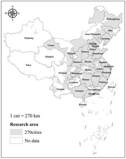
Figure 1.
Geographical location of 270 urban study areas in China. Note: Based on the standard base map of the standard map service system of the Ministry of Natural Resources (review number: GS (2016)1569), the base map was not modified (the same below).
2.2. Data Sources and Variable Selection
The explained variable was urban SO2 emissions, and the data on industrial SO2 emissions from prefecture-level cities in China were extracted from the 2019 China City Statistical Yearbook. Total industrial sulfur dioxide emissions in China were 4.47 million tons in 2018, declining 79.11% compared to 2007.
Air pollution is not determined by a single factor; it is the result of the joint action of socio-economic and natural conditions. Urban precipitation, ventilation coefficient, topography of urban terrain may influence SO2 emissions through the complex energy flows and material cycles in the ecosystem [33]. Obviously, human activities can generate SO2 through resource development, utilization, and consumption on the one hand, and can control SO2 pollution through environmental policies, technological innovation, and afforestation on the other [34].
Based on the pollution refuge hypothesis, Porter effect, environmental externality, Environmental Kuznets Curve, industrial structures, and the ecosystem, the natural and socioeconomic influencing factors could be fully considered [32]. The explanatory variables selected for this paper were urban precipitation (UP), ventilation coefficient (VC), topography of urban terrain (UT), per capita urban GDP (PGDP), population intensity (PI), the regional innovation and entrepreneurship level (RIE), foreign direct investment (FDI), financial development (FD), upgrading of industrial structures (UIS), research development investment (R&D), road construction (RC), and government intervention (GI). By selecting socio-economic and natural indicators, we aimed to explore the main factors affecting SO2 emission.
The indicators data of socio-economic data mainly obtained from the 2008 and 2019 China City Statistical Yearbook by calculation, were compiled by the National Bureau of Statistics of China and Statistical Bureau of each prefecture-level city. The calculation process is shown in Table 1. The data for the regional innovation and entrepreneurship level (RIE) were obtained from the Report of China Regional Innovation and Entrepreneurship Development Index by the National Development Research Institute of Peking University. Urban precipitation data (UP) were extracted from precipitation monitoring stations from the China Meteorological Data Network. Ventilation coefficient (VC) data were obtained from the product of wind speed and the atmospheric boundary layer height. Based on the ERA-interim database provided by the European center for medium-range weather forecasts (ECMWF), the raster data of prefecture-level cities in China were constructed. The indicator of topography of urban terrain(UT) was measured using GIS technology to extract a 1KM × 1KM raster at 1:1 million scale of China’s geographic digital elevation simulation data. See Table 1 for descriptive statistics involving the variables.

Table 1.
Variable description and index design.
2.3. Data Description
For some of the missing data, we calculated the missing values using linear interpolation. The relevant variable definitions are shown in Table 2.
Table 2.
Variable description.
2.4. Research Methodology
In this section, Moran’s I was used to represent the global agglomeration degree of SO2 emissions. Spatial kernel density was used to characterize the point aggregation degree of SO2 emissions. Hot spot analysis was used to characterize the local concentration of SO2 emissions. The standard deviation ellipse was used to represent the azimuth deviation of the spatial distribution of SO2 emissions. Through the above methods, we were able to reveal the spatial distribution and temporal and spatial evolution characteristics of SO2 emissions.
2.4.1. Spatial Autocorrelation
Waldo Tobler’s first law of geography is the spatial dependence of “proximity and similarity”: the closer the spatial distance, the stronger the correlation between elements. Spatial autocorrelation is often expressed by Moran’s I, Geary’s C, and Getis-Ord Gi*. Global Moran’s I was derived from the Pearson correlation. Positive values indicate positive spatial autocorrelation, while negative values indicate negative spatial autocorrelation, and the value range is between [–1, 1]. The calculation was designed as follows:
is the sample size, is the spatial weight matrix using inverse distance weights; and are the observations of spatial units and , is the average of the observations.
2.4.2. Spatial Kernel Density
Kernel density visualizes spatial aggregation by measuring the density of spatial elements within its periphery. The equation can be expressed as follows:
is the kernel density value at the point; is the kernel function; is the bandwidth; is the distance from the estimated point to sample .
2.4.3. Hot Spot Analysis
We used the high and low value area statistics of hot spot analysis (Getis-Ord Gi*) to measure the local agglomeration of cold–hot spots in the spatial distribution of urban SO2 emissions. The hot spot analysis could be estimated by the following equation:
In the equation, is the statistic of each spatial unit based on spatial distance weights , is the standardized statistic of the test; if the value is significantly positive, it indicates a hot spot agglomeration area, and the opposite is a cold spot agglomeration area. is the attribute values of spatial cells ; and are the mathematical expectation and coefficient of variation , respectively.
2.4.4. Standard Deviational Ellipse (SDE)
The evolutionary characteristics of geographic elements in two-dimensional spatial patterns were quantitatively revealed through the changing patterns of standard deviation ellipses. The process could be expressed by the following equation:
is the latitude and longitude of the geographic center of the city; is the attribute value of each city’s economic factors; is the weighted mean center; and are the standard deviations of the and axes, respectively.
2.4.5. Multiscale Geographically Weighted Regression Model (MGWR)
Multiscale geographically weighted regression (MGWR) was developed by Professor Stewart Fotheringham’s team [35,36]. The second law of geography assumes that spatial segregation causes the spatial localization and stratified heterogeneity of the study object. In this paper, we applied the multiscale geographically weighted regression model to explore the spatial heterogeneity of factors influencing SO2 emissions. The multiscale geographically weighted regression model could be estimated by the following equation:
represents the elasticity bandwidth of the regression coefficient of the variable ; is the central coordinate of the city location; and denote the intercept term and error term of the model, respectively. The impact factor coefficients β of the MGWR model were obtained based on the bandwidth of data differentiation, which was an improvement over the fixed bandwidth of classical GWR. In addition, the MGWR model uses the classical GWR quadratic kernel function and the AICc criterion to judge the degree of fit of the regression results.
Classical GWR is based on the weighted least squares estimation method, which is defined by the generalized additive linear model (GAM) [37]. In this paper, the initialization was based on the classical GWR estimation, which was fitted by the initialized residuals between the initially estimated predicted value and the true value.
(1) Classical GWR regression was conducted by residuals plus the first additive term and the first independent variable , which matched the best-fit bandwidth to obtain new residual and parameters to replace the original estimate. (2) The residual and of the second variable were replaced by regression of the new residuals plus the second additive term and the second independent variable . (3) Repeated as above up for the last variable (assuming k variables). (4) The above steps were a complete cycle, repeating the estimation until they reached the convergence criterion.
In this paper, the classical residual sum-of-squares variation ratio (RRS) was used as the convergence criterion. The equation could be expressed as follows:
indicates the sum of squared residuals from the previous step; indicates the sum of squared current residuals.
The metering software was MGWR2.2, downloaded from the School of Geosciences and Urban Planning at Arizona State University (https://sgsup.asu.edu/sparc/mgwr, accessed on 29 October 2021).
3. Results
3.1. Spatio-Temporal Evolution Distribution of SO2 Emissions
Figure 2 shows global Moran’s I of SO2 emissions in 270 Chinese cities in 2007 and 2018. By using the rook neighboring spatial matrix weights of GeoDa-1.18 software, the results showed that Moran’s I of SO2 emissions in 2007 and 2018 were 0.062 and 0.306, and the p-values for both were significantly positive at the level of 1%. Therefore, there were significant aggregation effect characteristics and a significant global autocorrelation of the SO2 emissions.
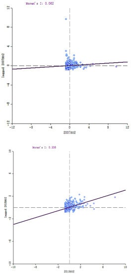
Figure 2.
Moran’s I of industrial SO2 emissions of 270 cities in 2007 and2018.
As shown in Figure 3, under the same reference concentration index, the total amount of SO2 pollution emissions from the 270 Chinese cities showed a declining trend from 2007 to 2018, and the spatial diffusion breadth and scale of the overall pollution emissions shrank. The average SO2 emissions reduced by 85.12% from 68,595,730 kg in 2007 to 10,209,440 kg in 2018. During the study period, SO2 emissions in the studied Chinese cities showed a spatial evolution feature from “ fragmentation of high emission” to “sporadic prominence of low emission “. Compared with 2018, most cities in China had higher SO2 emissions in 2007, such as Zhuhai (Guangdong province), Weifang (Shandong province), and Henan–Hengyang, and all of them exceeded 300,000,000 kg. There were 85 cities that discharged more than 80,000,000 kg, accounting for 31.48% of the total cities. In 2018, cities with SO2 emissions below 20,000,000 kg accounted for 67.41% of this total. As a result of the layouts of industries such as the steel and chemical industries, the SO2 emissions of Tangshan (Hebei province), Chongqing, Suzhou (Jiangsu province), and Weinan (Shaanxi province) cities all exceeded 80,000,000 kg. Due to the spatial patterns of emission changes, many cities of Shaanxi, Shandong, Zhejiang, Hunan, Yunnan, and Henan showed obvious emission reduction effects, but the SO2 emissions of some cities, such as Tangshan (Hebei province), Anshan (Liaoning province), Yuncheng (Shanxi province), Binzhou (Shandong province), Erdos, Baotou (Inner Mongolia), Wuxi (Jiangsu province), and Jiangmen (Guangdong province) had increased by more than 30,000,000 kg, showing a trend of increasing sporadic emissions that requires focused supervision and treatment.
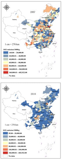
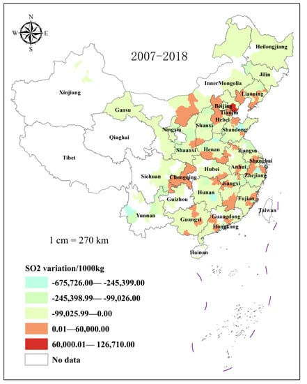
Figure 3.
Spatio-temporal evolution of SO2 emissions in 270 cities in 2007 to 2018.
3.2. Spatio-Temporal Clustering Characteristics of SO2 Emissions
We selected 2007 and 2018 as the study time points and used ArcGIS10.3 technology and the kernel density analysis method in the Spatial Analyst tool to extract urban surface elements as point elements.
During the study period, the spatial density of SO2 emissions decreased significantly, but the spatial layout changed little and remained consistent with the spatial distribution of SO2 emissions. Through a spatial kernel density analysis, the key control areas of SO2 emissions became obvious. The high-density areas of SO2 emissions in 2007 were mainly located in cities in Liaoning, Shandong, Shanxi, Henan, Shaanxi, Jiangsu, Anhui, Zhejiang, Jiangxi, Hubei, Hunan, Sichuan, Yunnan, and Guangdong provinces. The spatial density interval of SO2 emissions ranged from 0 to 40.32. In 2018, the high-density areas were distributed in cities in Liaoning, Hebei, Shandong, Shanxi, Henan, Jiangsu, Anhui, Zhejiang, Jiangxi, Chongqing, Guizhou, and Guangdong. The spatial density interval of SO2 emission ranged from 0 to 9.17. From the perspective of north–south geographical distribution, cities in the north were relatively contiguous and cities in the south were relatively scattered (see Figure 4).
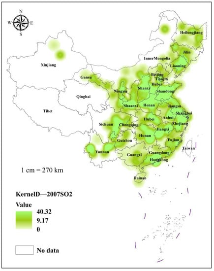
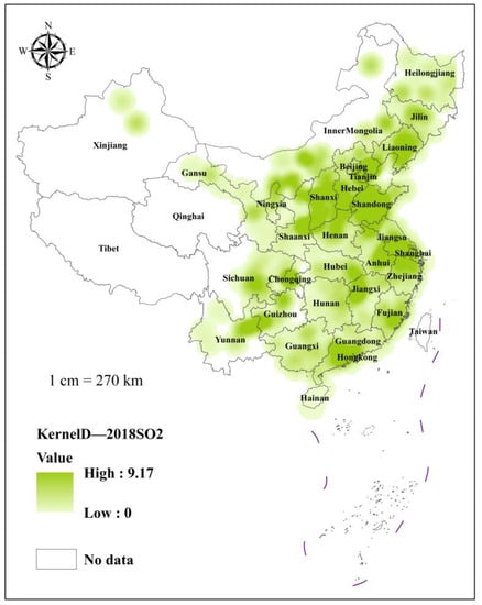
Figure 4.
Spatio-temporal evolution of SO2 emissions in 270 cities in 2007 and 2018.
The ArcGIS 10.3 software was used to perform the geographic distribution metrics and cluster distribution mapping of SO2 emissions through the standard deviation ellipse and hot spot analysis, respectively. The results of the standard deviation ellipse showed that the spatial distribution of SO2 emissions presented the “northeast–southwest” direction. From 2007 to 2018, the geographic distribution center of urban SO2 emissions moved in the northeast direction, from Zhumadian to Zhoukou in Henan Province. Further, the agglomeration effect of SO2 emissions became larger.
The results of the hot spot analysis showed that the hot spots and cold spots of SO2 emissions in the Chinese cities increased, and the hot spots gradually shifted from some sporadic cities in Shanxi, Hebei, and Yunnan to contiguous cities in Beijing, Tianjin, Hebei, Shanxi, Shandong, Inner Mongolia, and Jiangsu; the cold spots shifted from some cites in “Guangxi, Anhui” to contiguous cities in “Hubei, Gansu”, showing a polarization trend of “northern hot spots gathering, southern cold spots scattered”, which indicatedthat SO2 emissions of northern cities in China were in the development period of the differentiative effect(see Figure 5).
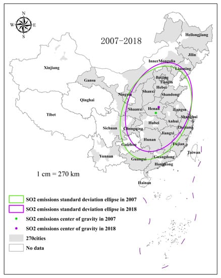
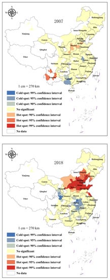
Figure 5.
Spatio-temporal evolution and hot spots of SO2 emissions in 270 cities in 2007 and 2018.
3.3. Analysis of Model Indicators
The previous paper introduced the variation pattern of SO2 emissions from spatial and temporal distribution and evolution. In this paper, we analyzed the influencing factors affecting SO2 emissions by comparing the advantages and disadvantages of the OLS, GWR, and MGWR models and selecting the appropriate model.
The results in Table 3 show that the regression results of MGWR were better than those of OLS and classical GWR. The sum of residual squares and the AICc value of the MGWR model test were smaller, while the goodness of R2 value was larger. The Akaike Information Criterion(AIC) or Akaike Information Criterion Corrected(AICc) and R2 value are a common standard used to judge the goodness of fit of regression models. The smaller the AIC and AICc value, the higher the R2 value and, thus, the higher the fitting degree of the model.
Table 3.
Comparison of OLS, Classic GWR, and MGWR fitting results.
According to the endowment characteristics of data, bandwidth selection showed spatial heterogeneity. The larger the bandwidth of the influencing factor, the stronger the applicability of the whole spatial scale. On the contrary, the smaller the bandwidth, the stronger the heterogeneity of the variable spatial scale. However, classical GWR has a fixed bandwidth value, which can only reflect the influence degree of the factor at the average spatial scale, which leads to estimation deviation with regard to the influencing factors. The MGWR model can automatically set different bandwidth values according to the characteristics of variables, which can fully reflect the spatial heterogeneity of influencing factors. Thereby, the MGWR model outperformed OLS and classical GWR. The following section analyzed the results from specific regressions.
3.4. Time-Series Analysis of Influencing Factors in Average Scale
From the results of the OLS method and the classic GWR model in Table 4, it can be concluded that the regression results of the factors were differential because the regression method used was different, and the classic GWR model was better than the OLS method. Comparing the results of classical GWR regressions from 2007 to2018 in the average spatial scale, the effectiveness of SO2 reduction was mainly the result of economic and social factors. As the urban per capita GDP grew, SO2 emissions declined year by year, but the impact has not been significant.
Table 4.
Results comparison of the average spatial scale model.
In 2007, in the average spatial scale, the influencing factors of SO2 emission reduction were industrial structure upgrading and government interventions. Further, the influencing factors of the increase in SO2 emissions in 2007 were foreign direct investment and research development investment. In 2018, the factors influencing the reduction in SO2 emissions were research development investment, population intensity, foreign direct investment, urban precipitation, and industrial structure upgrading, while the factors influencing the increase in SO2 emissions were government intervention and the regional innovation and entrepreneurship level. Therefore, the influencing factors of SO2 emissions at different time points differed, and the degree and direction of influence could change.
3.5. Spatial Heterogeneity of Influencing Factors
Taking SO2 emission reduction governance in Chinese cities in 2018 as an example, we analyzed the spatial multiscale stratification heterogeneity of influencing factors.
Foreign direct investment had a significant effect on SO2 emissions, showing a “pollution halo” emission reduction effect that decreased from Chinese northeast to southwest (see Figure 6a,b). Domestic enterprises could make use of the advanced technology and management models introduced by foreign capital to improve the total factor productivity of domestic enterprises. The model of low-carbon and green production and operation was able to reduce industrial SO2 emissions.
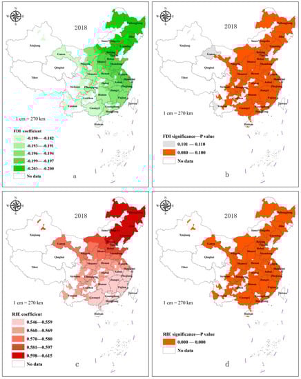
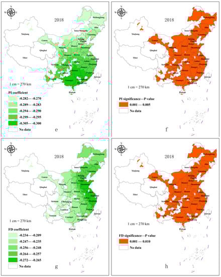
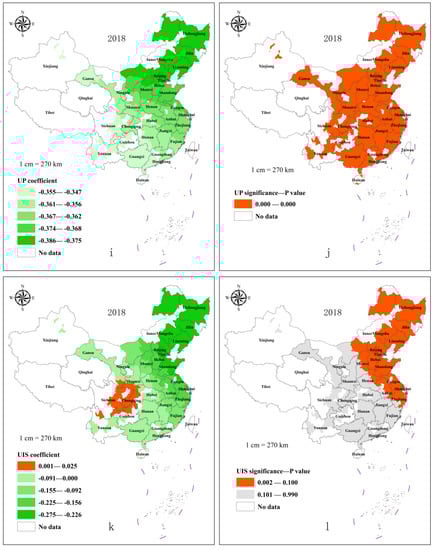
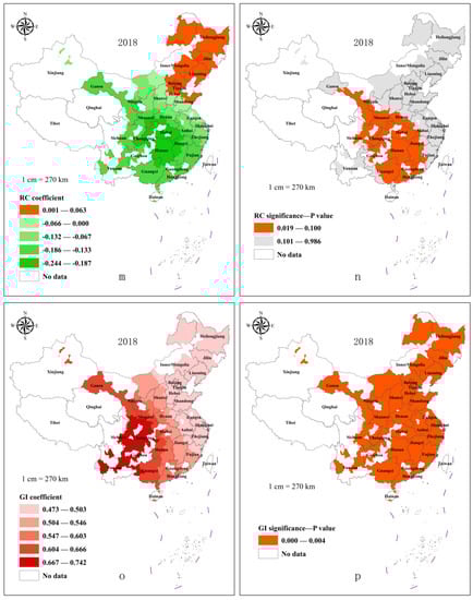
Figure 6.
Regression coefficient and significance spatial distribution of influencing factors of SO2 emissions in 270 cities in 2018. Note: (a,b), (c,d), (e,f), (g,h), (i,j), (k,l), (m,n), (o,p) represent the regression coefficient and significance level of FDI, RIE, PI, FD, up, UIS, RC, and GI, respectively.
The regional innovation and entrepreneurship level significantly increased SO2 emissions, with its effect being more significant in northern China than in southern China (see Figure 6c,d). This showed that the higher the level of urban innovation and entrepreneurship, the greater the promotion of economic development. In this way, the regional innovation and entrepreneurship level could accelerate the concentration of urban capital, resources, and technology; integrate the industrial and innovation chains of enterprises; also, promote the prosperity of the manufacturing industry. Industry developments cannot be separated from the massive consumption and utilization of resources, which leads to an increase in SO2 emissions for a short time.
Population intensity, financial development, and urban precipitation significantly reduced SO2 emissions (See Figure 6e–j). In China, the emission reduction effect of population intensity in southern cities was more significant than that in northern cities; the emission reduction effect of financial development and precipitation in eastern cities was better than that in central and western cities. Population intensity generated a strong agglomeration of the emission reduction effect. Financial development could effectively reduce SO2 emissions through the regulatory role investment and financing can play in influencing the speed, transformation, and scale of industrial development. The reduction in SO2 emissions through precipitation was due to a series of liquid-phase chemical reactions that form acidic compounds.
The upgrading of industrial structures had a significant impact on SO2 reduction in cities of northeast China, northern China, and eastern China, which accounted for 42.96% of the total sample (Figure 6k,l). The innovative green transformation of industrial development promoted the revitalization of the old industrial bases in northeast China and the rise of cities in the central region, and reduced the dependence on the “three high”(high pollution, high energy consumption, and high water consumption) industries, which also reduced SO2 emissions.
Urban road construction showed a significant impact on the increase in SO2 emissions in the southwest cities, accounting for 37.78% of the total sample (Figure 6m,n). The reason why SO2 emissions increased is that the large-scale construction of infrastructure directly drives the development of high-carbon emission industries, such as building materials, cement, steel, etc. In addition, road construction also indirectly led to an increase in vehicle consumption and fossil energy.
Government intervention significantly increased SO2 emissions, which was more obvious in cities of western China than in cities of northeast, northern, and eastern China (Figure 6o,p). Affected by central financial support and transfer payments, the economic development of cities in western China has been quite different from that of cities in eastern China. Large-scale investments, heavy chemical industry projects, infrastructure construction, and government intervention investments in China’s western development strategy promoted rapid economic development, but also increased SO2 emissions.
In addition, we found that the regression results for GDP per capita, the ventilation coefficient, research development investment, and the topography of urban terrain influencing SO2 emissions did not pass the significance test in the elastic spatial scale.
4. Discussion
4.1. Influencing Factors in Average and Multiscale Spaces
As was mentioned above, the factors influencing Chinese urban SO2 emissions were significantly differentiated and divergent on the spatial scale in 2018. We captured the main influencing factors of urban SO2 emissions using the mean values and statistical significance of coefficients. The main influencing factors of urban SO2 emissions were: the regional innovation and entrepreneurship level, government intervention, urban precipitation; the important factors were: population intensity, financial development, foreign direct investment; the minor factors were: industrial structure upgrading, road construction. Among these factors, the regional innovation and entrepreneurship level and government intervention were the main causes of increases in SO2 emissions, and the other influencing factors could reduce SO2 emissions(see Table 5).
Table 5.
Regression results of MGWR model.
4.2. Heterogeneity of Different Classification Dimensions
Since SO2 emissions are affected by various factors, such as geographic space, pollution level, resource endowment, and city scale, it was necessary to divide the study samples into different classification dimensions in order to analyze the influencing factors of the SO2 emissions. The regression results are shown in Table 6.
Table 6.
Regression results of MGWR model for geographical classification.
According to their geographical orientation, the 270 Chinese cities were divided into northern, southern, eastern, and central–western cities. The factors affecting SO2 emissions in China’s northern cities were government intervention, per capita GDP, the regional innovation and entrepreneurship level, research development investment, and urban precipitation. The factors affecting SO2 emissions in China’s southern cities were government intervention, the regional innovation and entrepreneurship level, population intensity, and financial development. The results of the geographic classification regression were generally consistent with the overall baseline regression, with southern cities showing a more pronounced emission reduction effect than northern cities. We also found that the increase in scientific research investment in northern Chinese cities was conducive to SO2 emission reduction.
The factors affecting SO2 emissions in Chinese eastern cities were regional innovation environment and urban precipitation, while the influencing factors affecting SO2 emissions in Chinese central and western cities were the regional innovation and entrepreneurship level, government intervention, road construction, financial development, population intensity, and foreign investment. The results showed that the means of SO2 emission reduction in central and western Chinese cities were more diversified than those in Chinese eastern cities. Therefore, under the natural geospatial classification, the main influencing factors affecting SO2 emission were different.
According to different dimensions of SO2 emission levels, resource endowment and urban population scales, the influencing factors affecting SO2 emission were explored. The regression results are shown in Table 7.
Table 7.
Regression results of MGWR model classified by different dimensions.
The sample cities were divided into high and low SO2 emissions groups according to their SO2 emissions mean values. The influencing factors of SO2 emissions were the regional innovation and entrepreneurship level, population intensity, the upgrading of industrial structures, and urban precipitation, which were consistent with the results of the baseline regression. Cities with high emissions of SO2 had more obvious emission reduction effects and more potential for a further reduction.
According to China’s State Council on the Issuance of National Sustainable Development Plan for Resource-based Cities (2013–2020) (Guo Fa (2013) No. 45), all the cities were further divided into resource-based cities and non-resource-based cities. The main influencing factor affecting SO2 emissions in resource-based cities was government intervention. The reason for this is that local officials focus on short-term urban economic development and highly rely on mineral resource development, resulting in the resource curse effect. The main influencing factors affecting SO2 emissions in non-resource-based cities were per capita GDP, the regional innovation and entrepreneurship level, government intervention, population intensity, and foreign direct investment. These results verified, once again, the baseline regression. In non-resource-based cities, the methods to reduce SO2 emissions were more diversified than those in resource-based cities.
5. Conclusions and Suggestions
In this paper, the spatial Moran index, kernel density, hot spot analysis, and standard deviation ellipse were used to analyze the spatio-temporal evolution characteristics of the SO2 emissions of 270 Chinese cities in 2007 and 2018. Based on the multiscale MGWR model, we quantitatively analyzed the influencing factors of SO2 emissions in 2018, and could draw the following conclusions:
- (1)
- During the study period, the SO2 emissions of 270 Chinese cities showed the spatial clustering effect, and the extent and scale of SO2 pollution declined significantly (by 85.12%). The overall spatial evolution presented a trend of SO2 emissions moving from “scattered and fragmented high emission” to “contiguous and extensive low emission”. The spatial density of SO2 emissions shifted from south to north in China, and the scope of agglomeration changed from 2007 to 2018.
- (2)
- The results of the standard deviation ellipse of 270 cities in China implied that the spatial distribution direction of SO2 emissions was “northeast–southwest”. The center of the SO2 emissions standard deviation ellipse shifted to the northeast, from Zhumadian City to Zhoukou City in Henan Province. The results indicated that the cold and hot spots of SO2 emissions in the studied Chinese cities all increased, showing a polarization trend of “hot spots gathering in the north and cold spots dispersing in the south”, while they also suggested that the SO2 emissions from the cities of China were still in the development period of the differentiative effect.
- (3)
- Regression results based on the MGWR model were more accurate than those estimated by OLS and classic GWR, and choosing different spatial bandwidths had different effects on the identification of influencing factors. The MGWR model screened out the main influencing factors of SO2 emissions: the regional innovation and entrepreneurship level, government intervention, and urban precipitation; the important factors: population intensity, financial development, and foreign direct investment; the minor factors: the upgrading of industrial structures and road construction. Among these factors, the regional innovation and entrepreneurship level and government intervention were found to be the main reasons for the increase in SO2 emissions, while the other influencing factors could contribute to the reduction in SO2 emissions.
- (4)
- Based on further spatial heterogeneity tests, the regression results were found to be consistent with the baseline regression as a whole. We refined our explanation of the causes of SO2 emissions in different types of cities, but there was also some spatial heterogeneity and uncertainty with regard to the role of influencing factors. For instance, the increase in scientific research investment in northern cities was found to be conducive to SO2 emission reduction. Due to the differences in development stages and lifestyles, the impact of per capita GDP on SO2 emissions in different cities was uncertain. For central–western and non-resource-based cities in China, the means of reducing SO2 emissions were more diversified.
Urban pollution management is a complex systematic project that is affected by the interaction between social economic activities and the natural ecological environment. The regression results of the MGWR model were more accurate and reliable than OLS and Classic GWR regression. It could carefully explore the urban spatial and heterogeneous impact of the main variables at each time point, clarify the focus on and the direction of SO2 emission reduction, and provide a scientific basis for decision-makers’ rational decision making and space governance. However, there are a number of research questions regarding SO2 emissions that can be further investigated in the future. For example, the research samples can be further reduced to the county level and enterprises. Factors such as temperature, solar radiation, vegetation coverage, environmental policy, and emission right markets should be considered. The spatially optimized layout of key governance areas will also be the direction of further research.
Author Contributions
W.Y.: methodology, software, data curation, writing original draft, and formal analysis; H.S.: conceptualization, supervision, project administration, resources and funding acquisition; Y.C.: writing—review and editing; X.X.: writing—review and editing. All authors have read and agreed to the published version of the manuscript.
Funding
This research was supported by the National Natural Science Foundation of China (no.71963030); Scientific and technological innovation project for doctoral students of Xinjiang University (project no.xjubscx−201922); 2018 “Silk Road” scientific research and innovation project for Postgraduates of School of economics and management of Xinjiang University (project no. jgsl18006).
Institutional Review Board Statement
Not applicable.
Informed Consent Statement
Not applicable.
Data Availability Statement
The study did not report any additional data.
Conflicts of Interest
The authors declare no competing interests.
References
- Zhao, Y.; Nielsen, C.P.; Lei, Y.; McElroy, M.B.; Hao, J. Quantifying the uncertainties of a bottom-up emission inventory of anthropogenic atmospheric pollutants in China. Atmos. Chem. Phys. 2011, 11, 2295–2308. [Google Scholar] [CrossRef] [Green Version]
- Wang, B.; Yu, M.; Zhu, Y.; Bao, P. Unveiling the driving factors of carbon emissions from industrial resource allocation in China: A spatial econometric perspective. Energy Policy 2021, 158, 112557. [Google Scholar] [CrossRef]
- Yuan, J.; Lu, Y.; Wang, C.; Cao, X.; Chen, C.; Cui, H.; Zhang, M.; Wang, C.; Li, X.; Johnson, A.C.; et al. Ecology of industrial pollution in China. Ecosyst. Health Sustain. 2020, 6, 1779010. [Google Scholar] [CrossRef]
- Zhang, S.; Li, D.; Ge, S.; Liu, S.; Wu, C.; Wang, Y.; Chen, Y.; Lv, S.; Wang, F.; Meng, J.; et al. Rapid sulfate formation from synergetic oxidation of SO2 by O3 and NO2 under ammonia-rich conditions: Implications for the explosive growth of atmospheric PM2.5 during haze events in China. Sci. Total Environ. 2021, 772, 144897. [Google Scholar] [CrossRef] [PubMed]
- Mazumdar, S.; Schimmel, H.; Higgins, I.T. Relation of daily mortality to air pollution: An analysis of 14 London winters, 1958/59–1971/72. Arch. Environ. Health 1982, 37, 213–220. [Google Scholar] [CrossRef] [PubMed]
- Benchrif, A.; Wheida, A.; Tahri, M.; Shubbar, R.M.; Biswas, B. Air quality during three COVID-19 lockdown phases: AQI, PM2.5 and NO2 assessment in cities with more than 1 million inhabitants. Sustain. Cities Soc. 2021, 74, 103170. [Google Scholar] [CrossRef] [PubMed]
- Liu, X.; Hadiatullah, H.; Tai, P.; Xu, Y.; Zhang, X.; Schnelle-Kreis, J.; Schloter-Hai, B.; Zimmermann, R. Air pollution in Germany: Spatio-temporal variations and their driving factors based on continuous data from 2008 to 2018. Environ. Pollut. 2021, 276, 116732. [Google Scholar] [CrossRef] [PubMed]
- Yang, W.T.; Qiao, P.; Liu, X.Z.; Lei, Y.L. Analysis of Multi-scale Spatio-temporal Differentiation Characteristics of PM2.5 in China from 2011 to 2017. Huan Jing KeXue 2020, 41, 5236–5244. [Google Scholar]
- Jin, N.; Li, J.; Jin, M.; Zhang, X. Spatiotemporal variation and determinants of population’s PM2.5 exposure risk in China, 1998–2017: A case study of the Beijing-Tianjin-Hebei region. Environ. Sci. Pollut. Res. Int. 2020, 27, 31767–31777. [Google Scholar] [CrossRef] [PubMed]
- Li, R.; Wang, Z.; Cui, L.; Fu, H.; Zhang, L.; Kong, L.; Chen, W.; Chen, J. Air pollution characteristics in China during 2015–2016: Spatiotemporal variations and key meteorological factors. Sci. Total Environ. 2019, 648, 902–915. [Google Scholar] [CrossRef] [PubMed]
- Yan, J.W.; Tao, F.; Zhang, S.Q.; Lin, S.; Zhou, T. Spatiotemporal Distribution Characteristics and Driving Forces of PM2.5 in Three Urban Agglomerations of the Yangtze River Economic Belt. Int. J. Environ. Res. Public Health 2021, 18, 2222. [Google Scholar] [CrossRef]
- Ron, S.; Dimitri, N.; Lerman Ginzburg, S.; Reisner, E.; Botana Martinez, P.; Zamore, W.; Echevarria, B.; Brugge, D.; Martinez, L.S.S. Health Lens Analysis: A Strategy to Engage Community in Environmental Health Research in Action. Sustainability 2021, 13, 1748. [Google Scholar] [CrossRef]
- Ren, L.; Matsumoto, K. Effects of socioeconomic and natural factors on air pollution in China: A spatial panel data analysis. Sci. Total Environ. 2020, 740, 140155. [Google Scholar] [CrossRef]
- Huang, X.G.; Zhao, J.B.; Cao, J.J.; Xin, W.D. Evolution of the Distribution of PM2.5 Concentration in the Yangtze River Economic Belt and Its Influencing Factors. Huan Jing KeXue 2020, 41, 1013–1024. [Google Scholar]
- Luo, Y.; Liu, S.; Che, L.; Yu, Y. Analysis of temporal spatial distribution characteristics of PM2.5 pollution and the influential meteorological factors using Big Data in Harbin, China. J. Air Waste Manag. Assoc. 2021, 71, 964–973. [Google Scholar] [CrossRef]
- Li, Z.; Yuan, X.; Xi, J.; Yang, L. The objects, agents, and tools of Chinese co-governance on air pollution: A review. Environ. Sci. Pollut. Res. Int. 2021, 28, 24972–24991. [Google Scholar] [CrossRef]
- Jia, R.; Fan, M.; Shao, S.; Yu, Y. Urbanization and haze-governance performance: Evidence from China’s 248 cities. J. Environ. Manag. 2021, 288, 112436. [Google Scholar] [CrossRef]
- Zhou, A.; Li, J. Analysis of the spatial effect of outward foreign direct investment on air pollution: Evidence from China. Environ. Sci. Pollut. Res. Int. 2021, 28, 50983–51002. [Google Scholar] [CrossRef]
- Liang, D.; Lee, W.C.; Liao, J.; Lawrence, J.; Wolfson, J.M.; Ebelt, S.T.; Kang, C.-M.; Koutrakis, P.; Sarnat, J.A. Estimating climate change-related impacts on outdoor air pollution infiltration. Environ. Res. 2021, 196, 110923. [Google Scholar] [CrossRef]
- Liu, J.Y.; Woodward, R.T.; Zhang, Y.J. Has Carbon Emissions Trading Reduced PM2.5 in China? Environ. Sci. Technol. 2021, 55, 6631–6643. [Google Scholar] [CrossRef]
- Liu, P.; Song, H.; Wang, T.; Wang, F.; Li, X.; Miao, C.; Zhao, H. Effects of meteorological conditions and anthropogenic precursors on ground-level ozone concentrations in Chinese cities. Environ. Pollut. 2020, 262, 114366. [Google Scholar] [CrossRef]
- Hemmati, F.; Dabbaghi, F.; Mahmoudi, G. Relationship between international tourism and concentrations of PM 2.5: An ecological study based on WHO data. J. Environ. Health Sci. Eng. 2020, 18, 1029–1035. [Google Scholar] [CrossRef]
- Ain, Q.; Ullah, R.; Kamran, M.A.; Zulfiqar, F. Air pollution and its economic impacts at household level: Willingness to pay for environmental services in Pakistan. Environ. Sci. Pollut. Res. Int. 2021, 28, 6611–6618. [Google Scholar] [CrossRef]
- Han, C.; Xu, R.; Zhang, Y.; Yu, W.; Zhang, Z.; Morawska, L.; Heyworth, J.; Jalaludin, B.; Morgan, G.; Marks, G.; et al. Air pollution control efficacy and health impacts: A global observational study from 2000 to 2016. Environ. Pollut. 2021, 287, 117211. [Google Scholar] [CrossRef]
- Kuo, P.F.; Putra, I.G.B. Analyzing the relationship between air pollution and various types of crime. PLoS ONE 2021, 16, e0255653. [Google Scholar] [CrossRef]
- Sarkodie, S.A.; Ahmed, M.Y.; Owusu, P.A. Ambient air pollution and meteorological factors escalate electricity consumption. Sci. Total Environ. 2021, 795, 148841. [Google Scholar] [CrossRef]
- Li, J.; Wang, N.; Wang, J.; Li, H. Spatiotemporal evolution of the remotely sensed global continental PM2.5 concentration from 2000–2014 based on Bayesian statistics. Environ. Pollut. 2018, 238, 471–481. [Google Scholar] [CrossRef] [Green Version]
- Jiang, W.; Gao, W.; Gao, X.; Ma, M.; Zhou, M.; Du, K.; Ma, X. Spatio-temporal heterogeneity of air pollution and its key influencing factors in the Yellow River Economic Belt of China from 2014 to 2019. J. Environ. Manag. 2021, 296, 113172. [Google Scholar] [CrossRef] [PubMed]
- Yu, Y.; Zhou, X.; Zhu, W.; Shi, Q. Socioeconomic driving factors of PM2.5 emission in Jing-Jin-Ji region, China: A generalized Divisia index approach. Environ. Sci. Pollut. Res. Int. 2021, 28, 15995–16013. [Google Scholar] [CrossRef] [PubMed]
- Gu, K.; Zhou, Y.; Sun, H.; Dong, F.; Zhao, L. Spatial distribution and determinants of PM2.5 in China’s cities: Fresh evidence from IDW and GWR. Environ. Monit. Assess. 2020, 193, 15. [Google Scholar] [CrossRef] [PubMed]
- Liu, N.; Zou, B.; Li, S.; Zhang, H.; Qin, K. Prediction of PM2.5 concentrations at unsampled points using multiscale geographically and temporally weighted regression. Environ. Pollut. 2021, 284, 117116. [Google Scholar] [CrossRef]
- Zhou, D.; Lin, Z.; Liu, L.; Qi, J. Spatial-temporal characteristics of urban air pollution in 337 Chinese cities and their influencing factors. Environ. Sci. Pollut. Res. Int. 2021, 28, 36234–36258. [Google Scholar] [CrossRef]
- Wang, P.; Cao, J.; Tie, X.; Wang, G.; Li, G.; Hu, T.; Hu, Y.; Xu, Y.; Xu, G.; Zhao, Y.; et al. Impact of Meteorological Parameters and Gaseous Pollutants on PM2.5 and PM10 Mass Concentrations during 2010 in Xi’an, China. Aerosol Air Qual. Res. 2015, 15, 1844–1854. [Google Scholar] [CrossRef] [Green Version]
- Yi, L.; Kang, Z.R.; Yang, L.; Musa, M.; Wang, F. Do driving restriction policies effectively alleviate smog pollution in China? Environ. Sci. Pollut. Res. Int. 2021, 28, 1–13. [Google Scholar]
- Fotheringham, A.S.; Yang, W.; Kang, W. Multiscale geographically weighted regression (MGWR). Ann. Am. Assoc. Geogr. 2017, 107, 1247–1265. [Google Scholar] [CrossRef]
- Oshan, T.M.; Smith, J.P.; Fotheringham, A.S. Targeting the spatial context of obesity determinants via multiscale geographically weighted regression. Int. J. Health Geogr. 2020, 19, 11. [Google Scholar] [CrossRef]
- Yang, Q.; Yuan, Q.; Li, T.; Shen, H.; Zhang, L. The Relationships between PM2.5 and Meteorological Factors in China: Seasonal and Regional Variations. Int. J. Environ. Res. Public Health 2017, 14, 1510. [Google Scholar] [CrossRef] [Green Version]
Publisher’s Note: MDPI stays neutral with regard to jurisdictional claims in published maps and institutional affiliations. |
© 2021 by the authors. Licensee MDPI, Basel, Switzerland. This article is an open access article distributed under the terms and conditions of the Creative Commons Attribution (CC BY) license (https://creativecommons.org/licenses/by/4.0/).