Article

Assessment of Climate Change Impacts on the Hydroclimatic Response in Burundi Based on CMIP6 ESMs

1
Department of Civil & Environmental Engineering, Sejong University, 209 Neungdong-ro, Gwangjin-Gu, Seoul 05006, Korea
2
Department of Hydrometeorology, Geographic Institute of Burundi (IGEBU), Bujumbura P.O. Box 331, Burundi
*
Author to whom correspondence should be addressed.
Sustainability 2021, 13(21), 12037; https://doi.org/10.3390/su132112037
Submission received: 15 September 2021 / Revised: 26 October 2021 / Accepted: 28 October 2021 / Published: 31 October 2021

Abstract

:
Burundi is susceptible to future water-related disasters, but examining the influence of climate change on regional hydroclimatic features is challenging due to a lack of local data and adaptation planning. This study investigated the influence of climate change on hydroclimate-focused changes in the climatology of heavy precipitation (and streamflow) means and extremes based on the multi-model ensemble mean of earth system models in the sixth phase of the Coupled Model Intercomparison Project (CMIP). For runoff analysis, hydrologic responses to future climate conditions were simulated using the Soil and Water Assessment Tool (SWAT) model over the Ruvubu River basin, Burundi. Temperature increases by 5.6 °C, with strong robustness, under future climate conditions. The mean annual precipitation (and runoff) undergoes large seasonal variations, with weak robustness. Precipitation (and streamflow) changes between the wet and dry seasons differ in signal and magnitude. However, alterations in both the amount and frequency of precipitation reveal the intensification of the water cycle due to anthropogenic climate change. Thus, the highest variability in the maximum daily streamflow is shown in months of long wet seasons, especially in the far future (2085). Without considering the regional climate characteristics and shared socioeconomic pathway (SSP) scenarios, this behavior is expected to be enhanced in 2085 (compared with 2045) and increase the severity of extreme precipitation and flood risk. Climate change will cause alterations in the magnitude and seasonal distributions of extreme precipitation (and streamflow). These findings could be important for flood planning and mitigation measures to cope with climate change in Burundi.

1. Introduction

Sub-Saharan Africa is plagued by frequent extreme water-related disasters such as floods and droughts as a result of global-scale atmospheric circulation and regional climate variability. For instance, global-scale tropical atmospheric circulation (i.e., Hadley circulation) in Sub-Saharan Africa, which leads to a twice-a-year seasonal migration, causes a substantial difference in precipitation between the wet and dry seasons. Concurrently, atmospheric circulation causes extreme climate events (i.e., heavy precipitation) resulting from interannual climate variations (i.e., El Niño–Southern Oscillation and Indian Ocean Dipole) in Sub-Saharan Africa [1,2,3,4,5]. Moreover, continuing changes in Earth’s climate system will enhance the probability of hard, prevalent, and irreversible impacts on humans and ecosystems across the globe (International Panel on Climate Change, IPCC) [6]. For Sub-Saharan Africa, climate projections show an increase in the variability of rainfall as the temperature rises, which might markedly affect the hydrological cycle [4,7,8]. An intensified hydrological cycle is considered to be the dominant factor influencing extreme climate events (e.g., storm surges, heavy precipitation, and floods) at both global and regional scales [7,9,10,11]. For this reason, it is imperative to examine potential influences of climate change on climate and hydroclimatic extremes over the Sub-Saharan African region.
To improve the understanding of these concerns in Sub-Saharan Africa, several studies have investigated the impacts of climate change on precipitation and runoff using outputs of the global climate model (GCM) or regional climate model (RCM) projections [12,13,14,15,16]. Most studies have predicted further increases in annual precipitation and enhanced spatial and temporal variations in precipitation under warmer conditions across Sub-Saharan Africa. However, the distribution of the change in annual precipitation is not the same as that of the change in seasonal precipitation. At the seasonal scale, Beyene et al. [12] suggested that the models project an increase in precipitation in the winter (DJF) season, while summer (JJA) precipitation increases or decreases according to the subregion in the Nile River Basin. Thus, changes in precipitation directly contribute to changes in runoff [11]. To understand the changes in runoff under future climate conditions, Elshamy et al. [13] assessed the annual mean changes in precipitation and evapotranspiration impact the streamflows of the upper Blue Nile based on ensemble GCMs. Liersch et al. [14] suggested an increase in the annual mean discharges as well as a shift in seasonal discharge with different change signals in the Upper Blue Nile catchment. These studies indicate that changes in temperature and precipitation will inevitably complicate water resource concerns (i.e., water availability and water-related disasters) on an annual scale as well as on a seasonal scale in Sub-Saharan Africa.
Among the many countries in Sub-Saharan Africa, Burundi is highly prone to be vulnerable to climate change. Burundi has experienced flood-related damage, including loss of life and property, due to heavy rainfall every year under the current climate [17]. Social and economic aspects of Burundi are essentially dependent on rain-fed agriculture, which sustains its economy and fast-growing population. More than 90% of the population lives in rural regions, where people are engaged in agricultural activities (the United Nations Framework Convention on Climate Change; UNFCCC) [18]. Therefore, the climate in Burundi plays the key role in controlling natural and human systems, including not only water resources, but also vegetation growth and food security [6,19]. In Burundi, to reduce catastrophic consequences induced by climate change, examining changes in hydroclimate as well as climate extremes under various climate change scenarios is necessary. However, a primary challenge for this region is that regional responses to future climate remain unknown, especially with respect to hydroclimate changes. Although previous studies on Burundi have suggested a high spatiotemporal variation in extreme events, this suggestion is based only on the observed precipitation data [7,17]. From a macro perspective, climate change affects various socioeconomic sectors of Burundi and has been surveyed solely by a research organization associated with the government agency in the form of a national report [18]. Several reports offer insight into the climate change effects in this area; however, they provide limited projections of hydroclimate changes in detail under the current global warming and likely future conditions.
The major objectives of this study are to assess the potential influence of climate change on hydroclimatic features and examine future extreme hydroclimate events (i.e., heavy precipitation and floods) considering regional seasonal climate features with a focus on Burundi (see Figure 1 and Figure 2). Figure 1 presents the flowchart of the study procedure. To improve the reliability of climate projections, we based the results on the multi-model ensemble mean (MME) of the Earth System Model (ESM) projections involved in the sixth phase of the Coupled Model Intercomparison Project (CMIP6) [20]. The degree of agreement between the multiple results is used to assess the confidence of climate projections, which will reflect the reliability of future projections of hydroclimatic variables [21,22]. Due to the coarse resolution of these ESMs, a statistical downscaling method (i.e., quantile mapping) was used to correct the biases recorded in the ESM outputs. Next, a hydrological model (the Soil and Water Assessment Tool (SWAT) model) was set up to simulate the streamflow of the Ruvubu River in Burundi. Here, we analyzed the long-term mean changes in hydroclimatic variables (e.g., precipitation and streamflow) to explore the regional hydroclimate effects of climate change. In particular, the focus of our study was on the hydroclimatic response to extreme precipitation (and runoff) changes which can cause floods, with consideration of seasonal distinctions and future climate conditions. To the best of our knowledge, no studies have assessed the potential impact of climate change on hydrological responses in Burundi. This study can provide various interconnected sectors with scientific information to alleviate the negative impacts of climate change on Burundi.

2. Materials and Methods
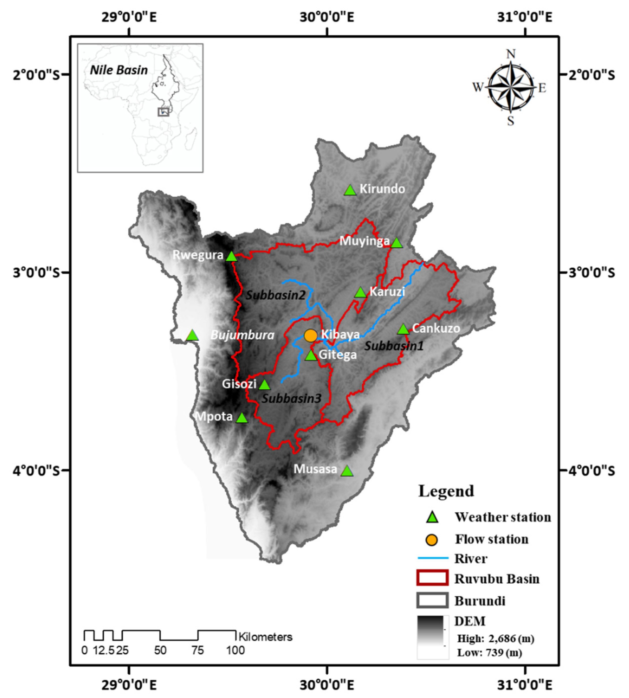
2.1. Study Area

Burundi is a landlocked country in Sub-Saharan Africa confined within latitudes 2.3° S–4.5° S and longitudes 29° E–31° E (Figure 2). The area of Burundi is 27,834 km2, and its elevation ranges from 739 m to 2686 m. Generally, the west, east, and northeast are lowlands, while the central, northern, and southern parts are highlands. Burundi is bordered to the west by the Democratic Republic of Congo (DRC), to the east and south by Tanzania, and to the north by Rwanda.
This study was conducted over a major part of the Ruvubu River basin located in the center of Burundi, as shown in Figure 2. The Ruvubu basin is delineated into three subbasins (subbasins 1, 2, and 3, including the main tributary of the Ruvubu River), and their characteristics are shown in Table 1. The length of the Ruvubu River is approximately 480 km, and the basin area is 9277.7 km2, which is approximately one-third of the total area of the country. The Ruvubu River joins the Akagera River in southern Rwanda and eventually joins the most distant southern part of the Nile River Basin.
The climate in Burundi can be broken down into two major seasons within a year, wet from October to May and dry from June to September (below 50 mm/month), with the annual mean precipitation between 800 mm and 1500 mm. However, Burundi typically experiences bimodal rainfall patterns in a year since the general circulation of the atmosphere in the Intertropical Convergence Zone (ITCZ), which is one of the main factors regulating rainfall seasonality, crosses Burundi twice a year [17,18]. There is an additional short dry season in January in the middle of the wet season (from October to May), which lasts for approximately 15 days. Therefore, the dry season is divided into two seasons: the long dry (June–July–August–September, JJAS) and the short dry (January, J) seasons [18]. Additionally, the wet season is divided into two seasons: the long wet (February–March–April–May, FMAM) and the short wet (October–November–December, OND) seasons. For Burundi, four subdivisions of the year, which are more commonly used to separate seasons, are implemented in this study. The precipitation over Burundi presents predominant seasonal variation (see the details in Section 4). The primary economic sector in Burundi is rain-fed agriculture, in which 90% of its inhabitants are employed. These seasonal climate features cause excessive rain in wet seasons and drought in dry seasons, which result in crop failure and food security risks [19]. Therefore, changes in precipitation will directly influence food security and water availability in this region. In particular, heavy rain recently affected Burundi as well as parts of neighboring Rwanda, where the loss of life and damage to structures increased due to heavy rain and flooding.
Figure 3 shows the spatial distributions of the long-term climatology (1985–2014) of four seasons (i.e., two wet seasons and two dry seasons) derived from 10 observation precipitation gauge data points across Burundi. One of the remarkable features of precipitation is its large variability both temporally and spatially. Individual seasonal precipitation features show somewhat greater variability across the region, even in the observations. The seasonal climate in Burundi is modified by altitude and is largely dominated by the general circulation of the atmosphere in the ITCZ, which is controlled by the convergence of trade winds [5,18]. However, differences in the mean monthly precipitation between long wet (FNAM), short wet (OND), and short dry (J) seasons are not clear in Figure 3.

2.2. Observational Climate Datasets

In this study, observational meteorological data were used to correct the biases in the climate model outputs and simulate streamflows for the Ruvubu basin. Observational meteorological stations were selected considering the availability of climate variables (i.e., minimum and maximum temperature, precipitation, relative humidity, solar radiation, and wind speed) and long-term observation data periods (1985–2014). Table 2 shows the information, including the annual mean climatology (e.g., maximum temperature, TMAX; minimum temperature, TMIN; and precipitation, PRE), from all the selected ten weather stations. A 10 weather gauge stations network for the whole area of Burundi was implemented in this study. In this network, only six gauge stations (i.e., No. 2–5, 9, and 10 suggested in Table 2) are located within the Rubuvu River basin. This six weather gauge stations network is equivalent to approximately one station every 39.3 km at the horizontal spatial resolution considering the catchment area (i.e., 9277.7 km2). Here is an assumption that each station is uniformly distributed in the basin. The observed weather data were obtained from the Geographic Institute of Burundi (IGEBU) at a daily timescale for the historical periods. In addition, geophysical datasets, which include DEM, soil, and land use/vegetation cover data, were collected from various sources and used to set up the hydrological model (i.e., the SWAT model) and simulate streamflows for the Ruvubu basin (see details in Section 2.4). The DEM data from the Shuttle Radar Topography Mission (SRTM) with a 1 arcsecond spatial resolution were obtained from the United States Geological Survey (USGS). Soil data with a 5 arcmin spatial resolution were collected from the Food Agriculture Organization (FAO) [23], and land use/vegetation cover data were collected from the Regional Centre for Mapping of Resources for Development (RCMRD, http://geoportal.rcmrd.org/, accessed on 15 September 2021). The observed discharge data were obtained from the IGEBU for the calibration and validation of the hydrological model parameters. The observed discharge data from the Kibaya station on the Ruvyironza River cover a period of 6 years (2012–2017). Data quality control was carried out before the application of these data (i.e., observational meteorological data and discharge data) in the analysis. Here, the QC process consisted of identifying problems in the data (e.g., outliers and missing values) and adjusting the data value under consideration of the various data features (e.g., regional climatology and spatiotemporal consistency).

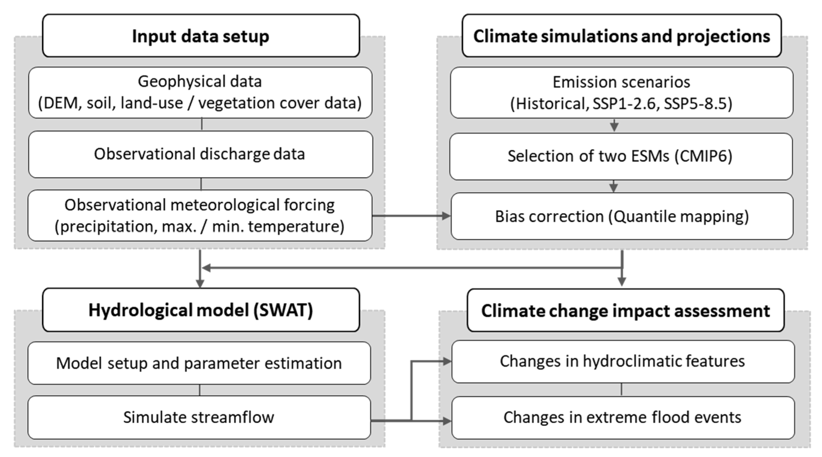
2.3. Climate Change Scenarios

To obtain reliable climate projections, we used MME projections based on the CMIP6. CMIP6 climate model simulations show improved regional characteristics when based on more complicated physical processes compared with the fifth phase of the CMIP climate model [24]. In this regard, analyses of the latest CMIP6 outputs based on an ESM can provide updated results and a better understanding of climate impacts on the hydroclimate in this region.
In this study, two ESMs (i.e., KACE-1-0-G and UKESM1-0-LL) in CMIP6 were implemented to examine the impacts of climate change on the hydrology of the Ruvubu basin. The two ESMs were selected in consideration of the availability of data (e.g., climate variables, various model runs, and different shared socioeconomic pathways) at the time of analysis and model performances. These ESMs reasonably simulate observations in a wide variety of contexts [25,26]. The KMA’s Advanced Community Earth system (KACE-1-0-G; K-ACE) model was developed by the National Institute of Meteorological Sciences/Korea Meteorological Administration (NIMS/KMA) in collaboration with the KMA–UK Met Office Hadley Centre. The K-ACE model is a coupled climate model (atmosphere–ocean–sea ice–land; AOIL), and detailed model descriptions were provided by Lee et al. [27]. Additionally, the UK Earth System Model (UKESM1-0-LL; UKESM1) implements a coupled climate model (i.e., HadGEM3-GC3.1) as a new core physical model with additional Earth system components (e.g., terrestrial carbon and nitrogen cycles) interactively coupled to each other. This model was jointly developed by the National Environmental Research Council (NERC) and the UK Met Office. Model runs were performed by the UK Met Office, the NIMS–KMA, and New Zealand’s National Institute of Weather and Atmospheric Research (see Sellar et al. [25] for details), and we used ensemble model runs performed by the NIMS–KMA among various model runs. To consider differences in initial conditions for individual model runs, climate change scenarios were derived from the three initial condition ensemble members (i.e., r1i1p1f1, r2i1p1f1, and r3i1p1f1 for KACE-1-0-G; r13i1p1f2, r14i1p1f2, and r15i1p1f2 for UKESM1) for every two ESM outputs. Climate model outputs under the historical scenario and two shared socioeconomic pathway (SSP) scenarios (i.e., SSP1-2.6 and SSP5-8.5) were obtained from the NIMS–KMA. SSP1-2.6 is at the low end of the range of future forcing pathways and is based on sustainability-focused growth and equality, whereas SSP5-8.5 is at the high end of the range of future forcing pathways and is based on the rapid and unconstrained growth of economic output and energy use.
Since the uncertainties in input forcing (e.g., maximum/minimum temperature and precipitation data) of the hydrological model are directly transferred to the uncertainties in runoff simulations, it is important to use reliable inputs to drive a hydrological model [28]. Due to the coarse resolutions of the climate projections from the ESMs for the local watershed, the downscaling technique is generally needed to adjust the global scale to the local scale and reduce the uncertainties recorded in the ESM outputs [28,29]. To remove biases in the input forcing data at a daily timescale, statistical bias correction was carried out by applying the quantile mapping (QM) method. The QM method is a simple and effective method to adjust biases by fitting the cumulative distribution function (CDF) of raw ESM outputs to that of observations. Therefore, it is commonly used in climate change impact studies [11,30,31,32]. The individual raw ESM outputs were downscaled to 10 observational weather stations located in the Ruvubu basin over Burundi (presented in Table 2).
After downscaling and bias correction of the ESMs, these models were validated. The validation consisted of calculating the bias for precipitation and temperature between the downscaled and bias-corrected MME mean and the observed long-term mean climatology. The MME was obtained by calculating the average mean monthly data for six ensembles of the two ESMs. In this study, to examine the future hydroclimatic response, future periods were set as two time slices of thirty years each, which are indicated as the near-term future period (2030–2059; S1) and the long-term future period (2070–2099; S2). The average variations in seasonal mean precipitation and temperature were compared to the reference period (1985–2014; S0) for two separate SSPs (SSP1-2.6 and SSP5-8.5).

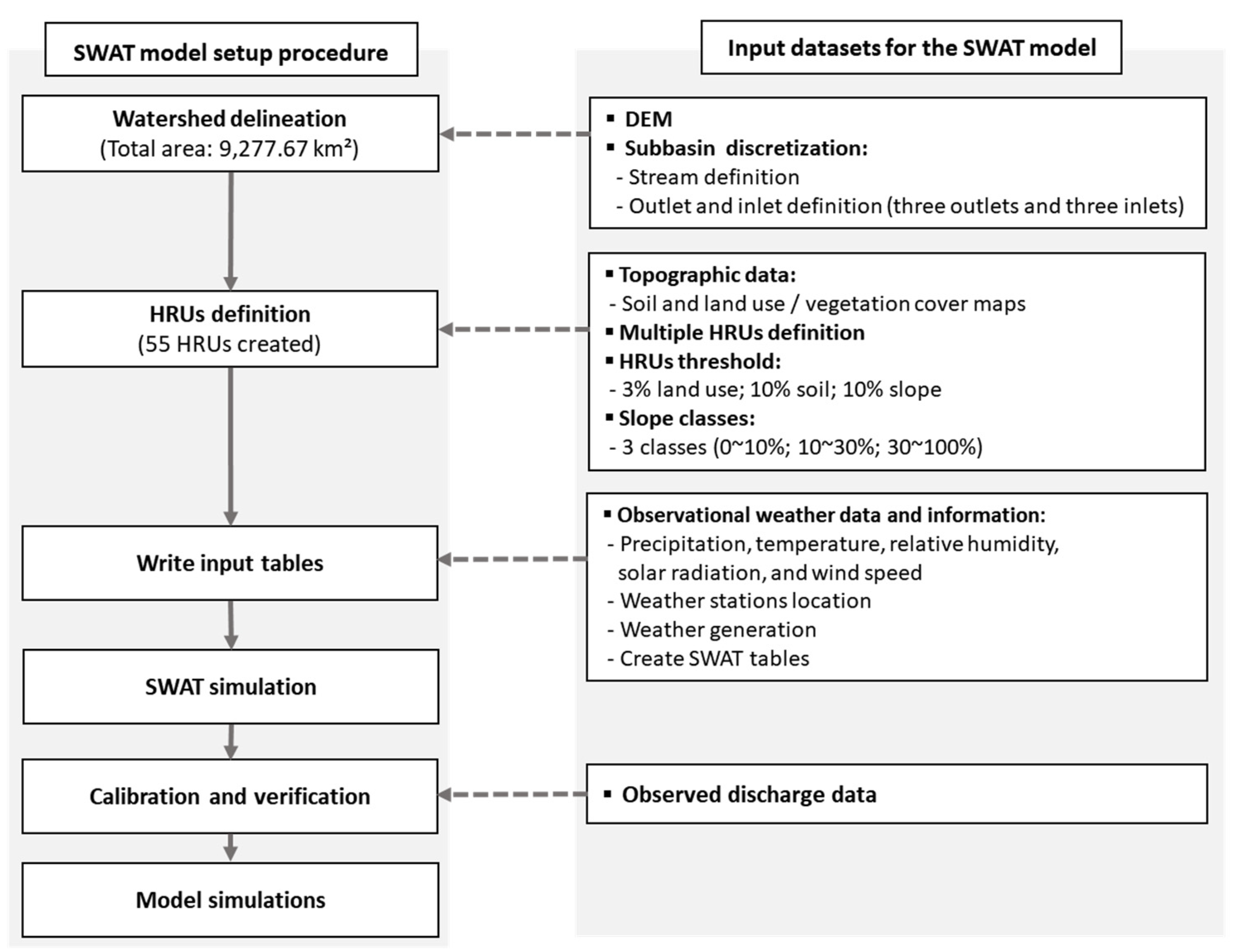
2.4. SWAT Hydrological Model

The SWAT model was developed by the Agricultural Research Service of the United States Department of Agriculture (USDA). The SWAT model is a continuous, semi-distributed, and process-based model that is operated on a daily basis at the basin scale [33,34]. It is widely used to simulate hydrological processes on various scales, including small catchments and large catchments, under different climate scenarios over a long period of time and is especially suitable for African river basins [35,36].
The SWAT model for the Ruvubu basin was set up by applying five key procedures using geophysical datasets (i.e., DEM and topographic data): watershed delineation, hydrologic response unit (HRU) analysis, write input tables, SWAT simulation, and parameter sensitivity analysis (see Appendix A). The DEM was used to delineate the watershed and analyze the drainage patterns of the land surface terrain. Topographic data (i.e., soil and land use/cover maps) were used for defining the distributions of HRUs in Burundi. Each subbasin was divided into HRUs considering topographic features on the basis of the land use/cover, soil, and slope feature. In the SWAT model, the hydrological cycle is simulated on the basis of the water balance equation at a daily timescale (Equation (1)):
S W t = S W 0 + i = 1 t P i Q i E i W i R i
where S W t (mm) is the final soil water volume, S W 0 (mm) is the initial soil water volume on day i , t (days) is the time, P i (mm) is the precipitation amount on day i , Q i (mm) is the amount of surface runoff on day i , E i (mm) is the evapotranspiration amount on day i , W i (mm) is the amount of water entering the unsaturated zone from the soil profile on day i , and R i (mm) is the amount of return flow on day i . Figure A1 shows a methodology flowchart for the SWAT setup in the Ruvubu basin.
Hydrological balance is simulated for each HRU based on the basic hydrological components such as evapotranspiration, soil water volume, surface runoff, lateral runoff, and groundwater runoff. In the SWAT, surface runoff and lateral runoff are simulated by the Soil Conservation Service (SCS) curve number (CN) method and kinematic storage model on a daily timescale, respectively. Individual hydrological components derived from the HRUs are summed up in each subbasin and then the components flow into the main channel of the subbasin. Channel runoff routing is estimated by the Muskingum method [33,34].
In the processes, individual hydrological components include the various model parameters. To simulate a realistic hydrological cycle, several model parameters are determined from basin features derived from geophysical data and river networks. Others are estimated for the certain HRUs in data-scarce regions from the transferred parameters estimated in the region with similar basin characteristics. After the model setup, the final step, which consisted of the calibration and validation processes, was conducted. Here, calibration and validation of the SWAT model were performed manually using observed discharge data at the Kibaya station on the Ruvyironza River, which is one of the tributaries of the Ruvubu River. The simulation results were highly influenced by the initial conditions (e.g., the initial soil conditions), especially in the data-scarce regions. Therefore, model runs were conducted during the period from 2010 to 2017 on a daily basis using observation meteorological forcing for calibration and validation processes, including two-year warm-up periods (2010–2011). Since the observation streamflow data are only available for four years (i.e., 2012 and 2015–2017), we separated the data period more weighted for the calibration rather than validation. Due to limited data availability, the recent data from 2015 to 2017 corresponding to the above-normal years (2015–2016) and the normal year (2017) were used for calibration, while the data for 2012, which was a normal year, were used for calibration. The SWAT parameters were calibrated considering the sensitivity of individual parameters (see details in [28,37]), which are displayed in Table 3.

3. Results

3.1. SWAT Hydrological Model Performance

To validate the simulated streamflows against the measured streamflows, the SWAT model was run based on observational meteorological input at a daily timescale (see Section 2.2). The simulated flow hydrographs from SWAT during the historical period (2012–2017) were compared with the measured streamflows during the same period except for 2 years (2013–2014) due to poor data quality. The streamflows simulated using observational meteorological input forcing are both quantitatively and qualitatively consistent with the measured streamflows of the Ruvyironza River basin (Figure 4a). The simulated streamflow captures the peaks and base flows of the measured streamflows for the calibration period as well as the validation period. Figure 4b presents box–whisker plots of daily streamflows in the Ruvyironza River basin on the basis of the measured streamflows (referred to as OBS) and simulated streamflows (referred to as SIM) forced by the observational meteorological input. SIM slightly overestimates the maximum OBS value during both the calibration and validation periods. The interquartile ranges represent the ability of SWAT to reasonably simulate the phase of the variation (i.e., lower quartile, median, and upper quartile) and high (and low) flows.
To statistically evaluate the accuracy of the simulated streamflows, we considered the coefficient of determination (R2), Nash–Sutcliffe efficiency (NSE), RMSE observation standard deviation ratio (RSR), and percent bias (PBIAS) as quantitative statistics. For daily data, the model performance was satisfactory: R2 > 0.50; NSE > 0.50; RSR < 0.70; and −25% < PBIAS < +25% [38]. The values of the four statistical indicators show that the model performance is reasonable in the calibration and validation periods (see Table 4). According to the positive PBIAS value, the SWAT model slightly overestimated the measured flows due to the uncertainties in various sources, such as the hydrological model, the uncertainty in the input data, and the lack of measured flow data. Overall, the results indicate that the SWAT model is applicable to simulating the water balance components over the Ruvubu basin.

3.2. Evaluation of the Climate Simulation

Prior to examining the hydroclimate response to potential climate change based on ESM ensemble projections, historical simulations were validated to confirm whether bias-corrected ESMs can suitably reproduce the fundamental climatological characteristics represented in the patterns observed in the Ruvubu basin. For the comparison during the historical period (1985–2014), the precipitation and temperature (i.e., maximum temperature and minimum temperature) data from individual gauge stations used in the SWAT model (Figure 2) were extracted from the six ESM ensembles and observation data. Hereafter, the results obtained from the MME of the six ESM ensembles and observations are referred to as MME and OBS, respectively.
Figure 5 presents the annual cycle of monthly temperature and precipitation from the MME and OBS over the Ruvubu basin. The monthly maximum and minimum temperatures in the MME are consistent with those in the OBS. The MME captures the typical shape of the annual cycle of OBS precipitation but tends to overestimate monthly precipitation. The positive bias in precipitation influences the error in the streamflow simulation. However, the MME adequately represents the seasonality of precipitation over Burundi. Regarding the magnitude of precipitation, the MME reproduces the precipitation seasonality in the OBS well, with a greater than 30-fold disparity between the wettest and driest months. The variation in precipitation between the six individual ESM outputs was determined. The inter-model spread varied in proportion to the magnitude of monthly precipitation. Therefore, the MME seems to overestimate precipitation. For the approach to seasonal precipitation, the magnitude of overestimation was higher in the months corresponding to the long dry season (JJAS) and lower in the months corresponding to the long wet season (FMAM). However, the range of precipitation in the ESM simulations was less than the interannual variability of the OBS in individual months, which was measured using the standard deviation during the historical period (1985–2014). Although the MME shows very good performance in capturing the monthly climatology of temperature rather than precipitation, these results demonstrate that the MME is capable of simulating the observed patterns in both temperature and precipitation.

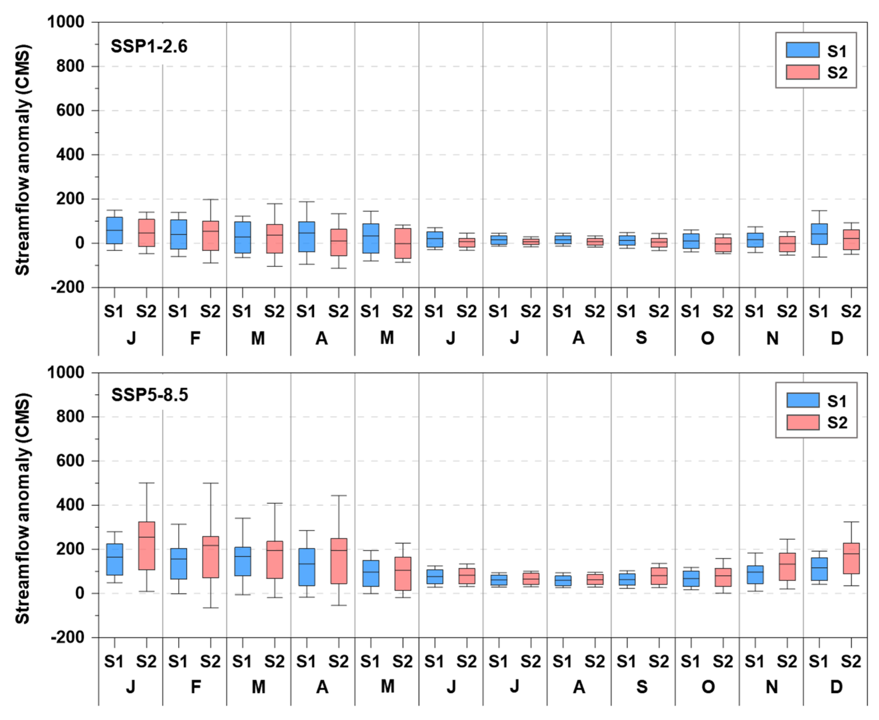
3.3. Future Projections of the Hydrologic Response

The different behaviors of temperature, precipitation, evapotranspiration, and runoff under warmer climates impact the annual (and seasonal) mean precipitation and runoff as well as their extremes. Table 5 shows the relative annual changes in the maximum temperature (TMAX), minimum temperature (TMIN), precipitation (PRE), actual evapotranspiration (AET), and total runoff (ROF) during the future periods (i.e., the near-future period, S1, and the far-future period, S2) in relation to the reference period based on the MME. The temperature increase is evident across the Ruvubu basin. The TMAX (and TMIN) is projected to increase in S1 by 1.95–2.29 °C and in S2 by 2.31–5.53 °C. The temperature response is very comparable to the variation in atmospheric greenhouse gas (GHG) concentration, suggesting that the levels of warming in SSP5-8.5 are much higher than those in SSP1-2.6. PRE is projected to increase by 9.15% (26.78%) in S1 and by 7.98% (38.01%) in S2 under SSP1-2.6 (SSP5-8.5). The ROF is projected to increase by 13.65% (62.16%) in the near future and by 4.94% (65.36%) in S2 under SSP1-2.6 (SSP5-8.5). The slower rate of increase in runoff during the S2 period than during the S1 period is caused by a significant increase in the AET compared with the increase in PRE. The MME-based relative changes in both PRE and ROF are slightly higher in the S1 period than in the S2 period, especially in SSP1-2.6.
Figure 6 illustrates the seasonal changes in the TMAX, TMIN, PRE, AET, and ROF. To evaluate the consistency among climate projections, we selected the regions where 100% and 67% of the projections agreed in terms of the sign of the change. This analysis highlights the confidence of projections. For temperature changes (i.e., TMAX and TMIN), the consistent patterns that are shown in the projections under the two SSPs are an increase in both dry seasons and in both wet seasons. The signals of the changes represented in most of the areas are likely robust, with four out of the six models in agreement (i.e., over 67%). Although the patterns and magnitudes of the changes differ seasonally, significant changes in the individual variables are shown under the higher SSP scenario (i.e., SSP5-8.5). In the majority of the seasons during individual future periods under both SSPs, the TMAX, TMIN, PRE, AET, and ROF in the future are higher than those in the reference period. It is probable that the increased temperatures (i.e., TMAX and TMIN) in response to enhanced GHG emissions are unequivocal during all seasons. However, even under the same global warming conditions, the modeled seasonal mean changes in PRE, AET, and ROF are very different from those in the TMAX and TMIN. Relatively, changes in PRE, AET, and ROF seem to be less consistent than the changes in temperature. However, the seasonal variations in PRE, AET, and ROF differ according to the SSPs (i.e., SSP1-2.6 and SSP5-8.5). Similar to the precipitation and runoff projections, the SSP5-8.5 projections predicted the largest change based on the MME. Moreover, the largest increases in the results under the two SSPs mostly occur in the far-future period (S2), and their statistical significance is limited for almost all variables except the TMAX and TMIN under SSP1-2.6.
Although the annual and seasonal behavior of precipitation shows a changed pattern in future climate conditions, more fundamentally, these features result from the enhancement of the hydrological cycle. Therefore, we examined how the enhanced hydrological cycle impacts precipitation on a daily scale in Burundi based on the frequency distribution of precipitation. To this end, we analyzed changes in the frequency distribution of daily precipitation during future periods compared with the reference period (referred to as the REF). Figure 7 shows the frequency distribution of daily precipitation at 10 stations based on the six ESM outputs for the two future periods and two different SSPs. Compared with the REF, the frequency of high-intensity precipitation increases for the future period. The relative change rate of both the frequency and amount of precipitation is individually calculated by the difference between the two future periods (S1 and S2) and the REF according to the individual intensity span. We counted all precipitation events and added up their amounts contributing to the individual intensity bin at an interval of 2 mm/day. These results imply the linkage between the change in the intensity of precipitation and the changes in total precipitation under future climate conditions. However, the ESM outputs show conflicting characteristics of precipitation according to the various intensity spans. An increase in high-intensity precipitation events occurs more frequently with the loss of a decrease in low-intensity precipitation events under warming conditions regardless of the future period and SSP scenario, as shown in Figure 8. This feature is one of the general results of intensification of the water cycle due to the anthropogenic climate. Although changes in both the amount and frequency of precipitation show relatively large variations under SSP1-2.6, they are clear and robust under SSP5-8.5. Moreover, this changing pattern becomes stronger in the S2 period under the high GHG emission scenario (i.e., SSP5-8.5) than under the low GHG emission scenario (i.e., SSP1-2.6). Thus, the precipitation change under SSP5-8.5 represents a drastic change in terms of both its amount and frequency across Burundi. These results reveal that changes in low-intensity and high-intensity precipitation may lead to increased drought and flood risk, respectively.
Figure 8 shows the box–whisker plot of anomalies in the monthly maximum daily streamflow between the REF and individual future periods (i.e., S1 and S2) in the Ruvubu basin. The monthly streamflow anomalies derived from the individual periods and the six ESM outputs during a future period were calculated based on the long-term mean of the maximum daily streamflow during the REF (1985–2014). Each box–whisker represents the temporal variability of the monthly maximum daily streamflow during the period. Similar change patterns of the monthly maximum daily streamflow are shown in the months (i.e., JJAS) corresponding to the long dry season regardless of the type of SSPs. However, in general, individual 30-year anomalies in the maximum daily streamflow respond differently to the GHG emission scenarios. The box–whisker plot of the monthly maximum daily streamflow under SSP1-2.6 shows relatively little difference between the S1 and S2 periods in terms of its variability except for some months (e.g., FMAM and D) compared to SSP5-8.5. Under SSP1-2.6, anomalies of the maximum daily streamflow in the S2 period are expected to decrease in the majority of months. However, under SSP5-8.5, anomalies of the maximum daily streamflow in the S2 period are expected to increase in all the months. Overall, the mean (and above median) value of each box–whisker tends to increase under SSP5-8.5 compared to that in the REF. The highest variability in the maximum daily streamflow during both the S1 and S2 periods is shown in several months (i.e., FMAM) corresponding to the long wet season, especially in the S2 period. These results reveal that flood risk will be exacerbated in future periods due to changes in hydrological elements according to climate change, particularly under high GHG emission conditions (SSP5-8.5).

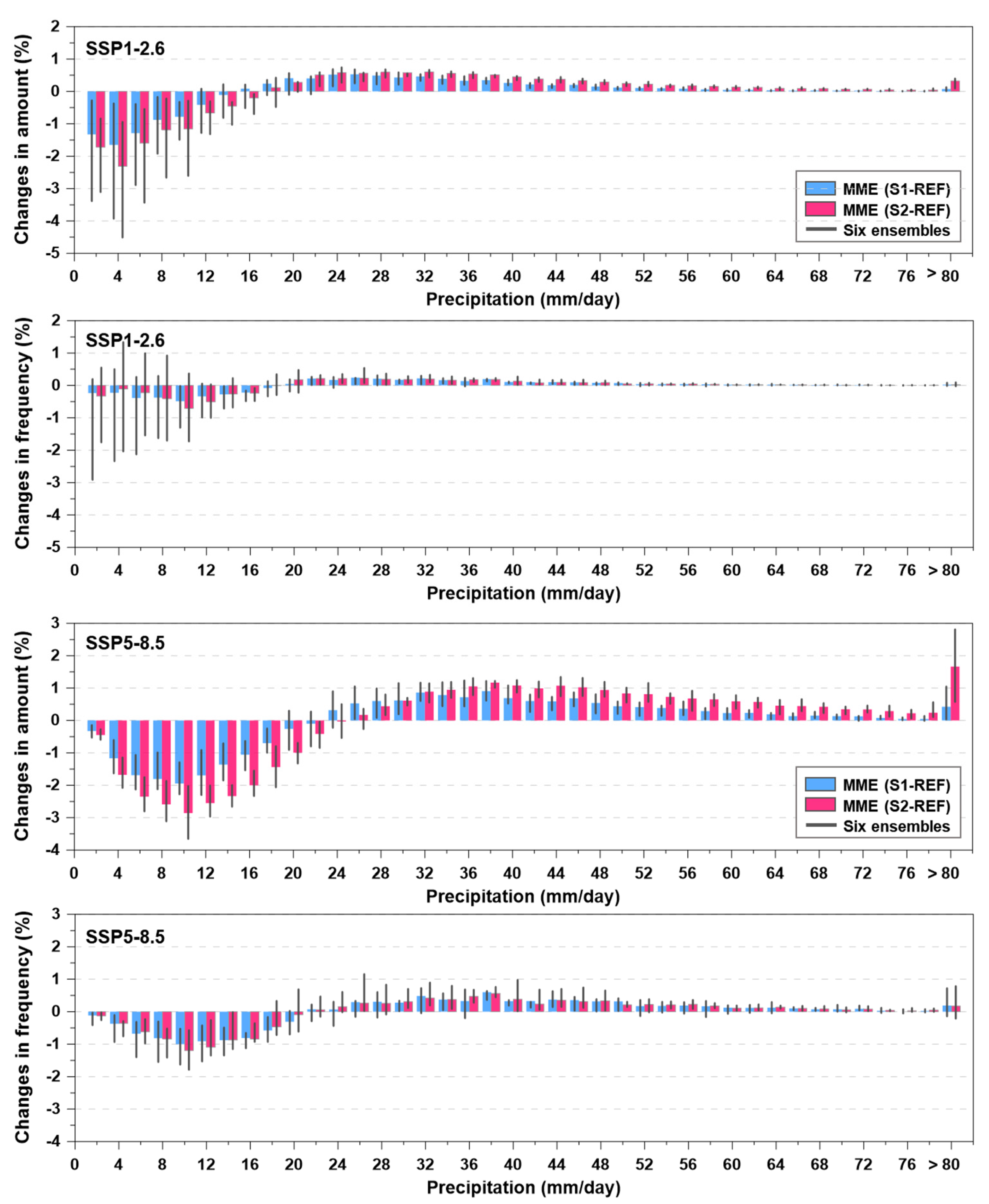
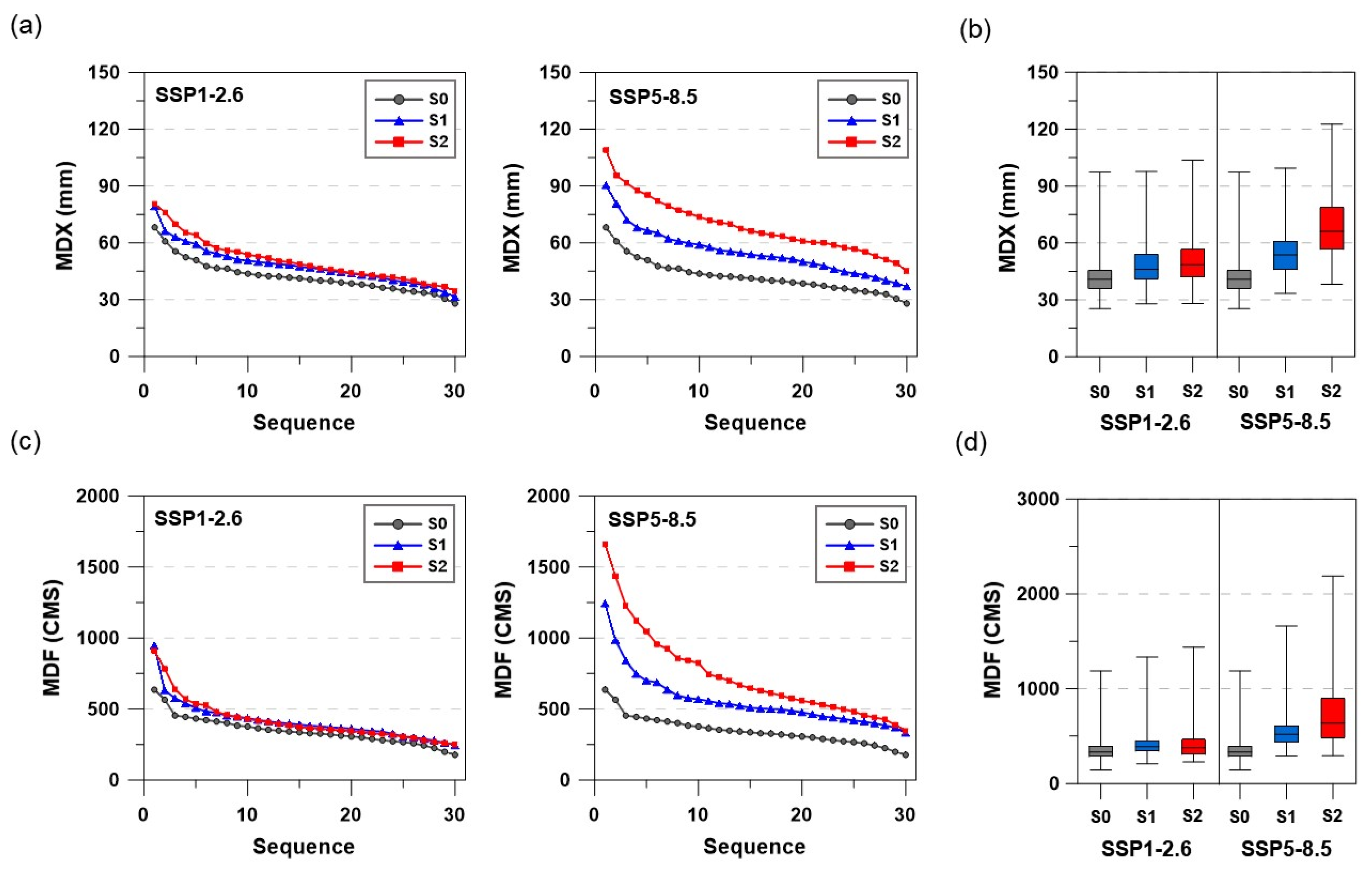
3.4. Future Projections of Extreme Flooding Events

We examined the future projections of extreme precipitation and extreme runoff derived from the SWAT simulations fed with the outputs of the six ensembles. Future changes were calculated based on the differences between the reference period (i.e., S0) and the two future periods (i.e., S1 and S2).
Figure 9 presents the changes in extreme events derived from the annual maximum precipitation and the annual maximum streamflow for the 30 years of the individual reference period and two future periods. To investigate the extent to which the SSP1-2.6 and SSP5-8.5 scenarios affect the severity of extreme precipitation and streamflow, we compared both the annual maximum daily precipitation (MDX) and the annual maximum daily streamflow (MDF) over the Ruvubu basin. Figure 9a (and Figure 9c) shows the 30 MDXs (and MDFs) in ascending order during the individual 30-year periods according to the historical and SSP (SSP1-2.6 and SSP5-8.5) scenarios. The MDX shows considerable interannual variability, with values ranging from below 30 mm to above 105 mm. The increases in the magnitude of the MDX (and the MDF) in the S1 and S2 periods are strongly connected with the relatively high MDX (and MDF) values among sequences of the 30-year values. On the other hand, the future period seems to have slightly influenced the lower MDF values, especially in SSP1-2.6. However, the MDX (and the MDF) is projected to increase in all sequences under SSP5-8.5, and the largest increases are the maximum values. In addition, the increasing trend in the MDX (and the MDF) is more apparent under SSP5-8.5 than under SSP1-2.6 regardless of ESM outputs (Figure 9b,d). The results imply that future climate is highly likely to increase flood extremes and accompanying risks in the Ruvubu basin.
To analyze the disparity in the seasonal occurrences of the MDX and the MDF, the absolute seasonal frequency of the individual MDX and MDF values for each period (i.e., S0, S1, and S2) is represented in Figure 10. Figure 10 indicates that changes in the MDX and MDF frequency are related to their seasonal distribution. The increase in the frequency of the MDX during L.WET and the decrease in the frequency of the MDX during L.DRY and S.WET contribute to the higher occurrence of the MDX during L.WET for the S1 period. Moreover, the increase in the frequency of the MDX during S.WET and the decrease in the frequency of the MDX during L.WET and L.DRY contribute to the higher occurrence of the MDX during S.WET in the S2 period. In general, larger seasonal changes in the MDX and the MDF are shown under SSP5-8.5 than under SSP1-2.6. This result indicates that future climates cause a redistribution of the seasonal frequencies of the MDX and the MDF.

4. Discussion

The influence of climate change on regional features of temperature is straightforward, whereas the impacts on the features of hydrological variables are ambiguous due to strong natural variability [39]. Therefore, temporal and spatial variability in precipitation is a critical climatic factor for regulating society, water resources, agriculture, the environment, and water-related disasters in a region [40,41]. Moreover, the precipitation in Sub-Saharan Africa is particularly heterogeneous, resulting from the complexity of topography, water/land distribution, maritime effects, and seasonal dynamics [2]. Notably, the temporal and spatial characteristics of precipitation are heterogeneous among the countries in Sub-Saharan Africa, especially Burundi (see Figure 3). However, seasonal precipitation patterns show bimodal regimes (see Figure 5). The rainfall peaks (e.g., larger than 165 mm/month based on the MME) are generally concentrated in the months of the long wet (FMAM) and short wet seasons (OND). On the other hand, a small amount of precipitation is found in the months of the long dry season (JJAS), whereas it is not clear in those of the short dry season (J). The short dry season (J) varies in length and is related to the dry spell lengths rather than the amount of monthly precipitation. Therefore, the precipitation variability in Burundi makes it difficult to manage water resources and deal with water-related disasters in an effective way under the current climate conditions.
However, robust responses of an intensified hydroclimatic regime with increased high-intensity precipitation have been suggested at the global and regional scales [39], which is in line with these results in Burundi (e.g., Figure 7 and Figure 9a,b). The increase in extreme climate events will have adverse effects on flooding rather than drought in Burundi (e.g., Figure 8, Figure 9 and Figure 10). In general, water-related disasters result in regional extreme precipitation. The annual maxima of precipitation, which are recognized as the criterion for determining the magnitudes of extreme precipitation events, are characterized by distinct seasonal regional climate variability at the local scale [42]. In Burundi, extreme precipitation events are impacted by different meteorological factors, i.e., a combination of local factors and enhanced air moisture from the Indian Ocean and the presence of the mesoscale convective vortex [5]. Burundi usually experiences extreme precipitation events in two wet seasons (i.e., S.WET and L.WET) during the REF period (Figure 10), which is in line with previous studies [5,17]. Climate change will increase the amount and frequency of high-intensity precipitation for future periods (Figure 7). In addition, for the far-future period (i.e., S2; 2085), the extreme streamflow will be likely to increase in most of the months (i.e., corresponding to S.WET, L.WET, and S.DRY) (Figure 8). The results indicate that further climate change is likely to increase the variety of extreme events (i.e., the MDX) at the temporal scale and the risk of floods with more intense extreme precipitation in Burundi.
Changes in the climate system originating from emissions of GHGs are expected to transform runoff and extreme runoff patterns. In particular, climate adaptation related to water-related disasters, which disrupt the economies of developing countries, is more important than other aspects to minimize damage. Therefore, the hydrological model has been generally used for simulating runoff and investigating the potential changes in runoff under possible future climate scenarios [11,43]. However, despite this foreseeable relevance and the widespread applicability of hydrological modeling, hydrological impact assessments under climate change have received little attention in Burundi. Hydrological modeling is still a major challenge in some regions, including Burundi, due to data availability (i.e., accessibility of data, lack of reliable data, and missing data) and sparsity of gauge data across time and space for observing runoff features [44,45,46]. The biggest and fundamental problem is that the observation period of the discharge data is too short for estimating the SWAT model parameters. It may contribute to the main uncertainty source of streamflow simulation. Due to these reasons related to the local data, the limitation of this study is that uncertainties are involved in simulating the streamflow in the Ruvubu River basin. Although various uncertainties are associated with simulating runoff under climate change variations (i.e., systematic biases between the ESMs and observations, variations among the ESMs and emission scenarios), Burundi is likely to face challenges in coping with extreme runoff and concurrent streamflow under global warming. Therefore, our results indicate that further research on flood planning techniques and the implementation of adaptation and mitigation measures to address climate change could be necessary for this region.

5. Conclusions

To our knowledge, except for some national reports, few studies have conducted a climate change impact assessment on the hydroclimate over the Burundi region. In Burundi’s water resource management, one of the primary challenges is hydroclimate variability. Therefore, this study investigated the hydroclimatic response (i.e., the mean climatology and extreme events) to climate change based on the MME forced by two SSP (SSP1-2.6 and SSP5-8.5) scenarios and CMIP6 ESM simulations in the Ruvubu basin in Burundi from a seasonal perspective. After removing systematic biases, six ESM climate projections were used as meteorological forcing for the SWAT model to simulate the streamflow across the Burundi river basin. To obtain reliable streamflow simulations, the SWAT model was calibrated and validated using the observational datasets in Burundi. Future changes in hydroclimate variables (e.g., TMAX, TMIN, PRE, and ROF) were calculated by comparing the differences between individual future climate conditions (S1 and S2 periods under the two SSPs) and the reference period. The focus of this study was a comparison of hydroclimatic responses to potential future climate in terms of their seasonal means, characteristics, and extremes.
The annual mean changes in all of the hydroclimate variables (e.g., TMAX, TMIN, PRE, AET, and ROF) except for TMIN during the S1 period are much larger for the two future periods (S1 and S2) under SSP5-8.5 than under SSP1-2.6. The annual mean changes in both PRE and ROF during the S2 period show lower increases than during the S1 period under SSP1-2.6. Meanwhile, changes in other hydroclimate variables show intensified hydrological response in a future period (i.e., S2 period; 2085). From a seasonal point of view, the seasonal means of the TMAX (and TMIN) will similarly increase by 1.7–2.4 °C (1.7–2.2 °C) in all the four seasons (i.e., S.DRY, L.WET, L.DRY, and S.WET) during the S1 period regardless of the SSP scenario (see Table 5). However, a larger difference (i.e., approximately 2.9–3.6 °C) between the two SSPs is shown for both TMAX and TMIN during the S2 period due to the impact of high cumulative GHGs by the end of the twenty-first century. The potential changes in the TMAX and TMIN are more obvious and robust (with six out of six ensemble models in agreement) than those in other hydroclimate variables. In line with the expected increases in the TMAX and TMIN, the seasonal mean changes in the AET during the S1 period (i.e., approximately –2.8–6.8%) compared with the S2 period (i.e., approximately 7.7–54.9%) slightly differ between SSP1-2.6 and SSP5-8.5. However, individual seasonal changes in PRE and ROF are quite different in the two future periods and two SSP scenarios. The changes in PRE (and ROF) are dominated by various factors, including not only the global temperature rise but also the localized natural variability. Regarding the precipitation extremes, adaptation to enhanced heavy precipitation (measured by the MDX) in terms of both magnitude and seasonal occurrence will be necessary for Burundi. The magnitudes of the MDX and the MDF are projected to increase more in future periods, especially during the S2 period under SSP5-8.5, than during the reference period.
The results of this investigation reveal that future climate change will impact the mean climatology (i.e., the annual mean and the seasonal mean) as well as the extreme values of hydroclimate variables (e.g., TMAX, TMIN, PRE, AET, and ROF) with a certain level of reliability in the Burundi region. In addition, changes in precipitation extremes increase the risks related to flood extremes and damage socioeconomic sectors. Moreover, the daily maximum runoff, which is likely to increase the flood risk, increases in the future period irrespective of the type of climate projection. As suggested in this study, the climate of Burundi is highly influenced by climate change, similar to other countries in Sub-Saharan Africa. Therefore, understanding the long-lasting impacts of global warming on the mean changes in hydroclimate is critical to the planning of water resource management and increasing agricultural production in Burundi. Structural and nonstructural measures for water-related disasters are needed to adapt to climate change, especially to minimize the potential flood risk in Burundi.

Author Contributions

Conceptualization, J.-B.K. and J.d.D.H.; methodology, J.-B.K. and J.d.D.H.; software, J.-B.K. and J.d.D.H.; validation, J.d.D.H. and S.-H.K.; formal analysis, J.-B.K. and J.d.D.H.; investigation, J.d.D.H. and S.-H.K.; resources, J.d.D.H.; data curation, J.d.D.H. and S.-H.K.; writing—original draft preparation, J.-B.K. and J.d.D.H.; writing—review and editing, J.-B.K., S.-H.K., and D.-H.B.; visualization, J.-B.K. and J.d.D.H.; supervision, D.-H.B.; project administration, D.-H.B.; funding acquisition, D.-H.B. All authors have read and agreed to the published version of the manuscript.

Funding

This work was supported by the Korea Environmental Industry & Technology Institute (KEITI) through the Water Management Research Program funded by the Korea Ministry of Environment (MOE) (130747) and the Ministry of Science and ICT of the Republic of Korea.

Institutional Review Board Statement

Not applicable.

Informed Consent Statement

Not applicable.

Acknowledgments

The authors send thanks to the guest editors and all anonymous reviewers for valuable comments and suggestions. This work was supported by the Korea Environmental Industry & Technology Institute (KEITI) through the Water Management Research Program funded by the Korea Ministry of Environment (MOE) (130747) and the Ministry of Science and ICT of the Republic of Korea.

Conflicts of Interest

The authors declare no conflict of interest.

Appendix A

Figure A1. Flowchart of the SWAT setup in the Ruvubu River basin.
Sustainability 13 12037 g0a1

References

  1. Cai, W.; Santoso, A.; Wang, G.; Weller, E.; Wu, L.; Ashok, K.; Masumoto, Y.; Yamagata, T. Increased frequency of extreme Indian Ocean Dipole events due to greenhouse warming. Nat. Cell Biol. 2014, 510, 254–258. [Google Scholar] [CrossRef] [PubMed]
  2. Nicholson, S.E. Climate and climatic variability of rainfall over eastern Africa. Rev. Geophys. 2017, 55, 590–635. [Google Scholar] [CrossRef] [Green Version]
  3. Ummenhofer, C.C.; Kulüke, M.; Tierney, J. Extremes in East African hydroclimate and links to Indo-Pacific variability on interannual to decadal timescales. Clim. Dyn. 2018, 50, 2971–2991. [Google Scholar] [CrossRef] [Green Version]
  4. Endris, H.S.; Lennard, C.; Hewitson, B.; Dosio, A.; Nikulin, G.; Artan, G.A. Future changes in rainfall associated with ENSO, IOD and changes in the mean state over Eastern Africa. Clim. Dyn. 2018, 52, 2029–2053. [Google Scholar] [CrossRef] [Green Version]
  5. Nkunzimana, A.; Bi, S.; Alriah, M.A.A.; Zhi, T.; Kur, N.A.D. Diagnosis of meteorological factors associated with recent extreme rainfall events over Burundi. Atmospheric Res. 2020, 244, 105069. [Google Scholar] [CrossRef]
  6. IPCC. Climate change 2014: Synthesis report. In Contribution of Working Groups I, II and III to the Fifth Assessment Report of the Intergovernmental Panel on Climate Change; Pachauri, R.K., Meyer, L.A., Eds.; IPCC: Geneva, Switzerland, 2014. [Google Scholar]
  7. IPCC. Summary for Policymakers. In Global Warming of 1.5°C; An IPCC Special Report on the impacts of global warming of 1.5 °C above pre-industrial levels and related global greenhouse gas emission pathways, in the context of strengthening the global response to the threat of climate change, sustainable development, and efforts to eradicate poverty; Masson-Delmotte, V., Zhai, P., Pörtner, H.-O., Roberts, D., Skea, J., Shukla, P.R., Pirani, A., Moufouma-Okia, W., Péan, C., Pidcock, R., et al., Eds.; World Meteorological Organization: Geneva, Switzerland, 2018. [Google Scholar]
  8. Gebrechorkos, S.H.; Bernhofer, C.; Hülsmann, S. Climate change impact assessment on the hydrology of a large river basin in Ethiopia using a local-scale climate modelling approach. Sci. Total Environ. 2020, 742, 140504. [Google Scholar] [CrossRef] [PubMed]
  9. Trenberth, K.E. Conceptual Framework for Changes of Extremes of the Hydrological Cycle with Climate Change. Clim. Chang. 1999, 42, 327–339. [Google Scholar] [CrossRef]
  10. IPCC. Climate Change 2013: The Physical Science Basis; Contribution of Working Group I to the Fifth Assessment Report of the Intergovernmental Panel on Climate Change; Stocker, T.F., Qin, D., Plattner, G.-K., Tignor, M., Allen, S.K., Boschung, J., Nauels, A., Xia, Y., Bex, V., Midgley, P.M., Eds.; Cambridge University Press: Cambridge, UK, 2013; p. 1535. [Google Scholar]
  11. Kim, J.; Im, E.; Bae, D. Intensified hydroclimatic regime in Korean basins under 1.5 and 2°C global warming. Int. J. Clim. 2020, 40, 1965–1978. [Google Scholar] [CrossRef]
  12. Beyene, T.; Lettenmaier, D.P.; Kabat, P. Hydrologic impacts of climate change on the Nile River Basin: Implications of the 2007 IPCC scenarios. Clim. Chang. 2010, 100, 433–461. [Google Scholar] [CrossRef]
  13. Elshamy, M.E.; Seierstad, I.A.; Sorteberg, A. Impacts of climate change on Blue Nile flows using bias-corrected GCM scenarios. Hydrol. Earth Syst. Sci. 2009, 13, 551–565. [Google Scholar] [CrossRef] [Green Version]
  14. Liersch, S.; Tecklenburg, J.; Rust, H.; Dobler, A.; Fischer, M.; Kruschke, T.; Koch, H.; Hattermann, F.F. Are we using the right fuel to drive hydrological models? A climate impact study in the Upper Blue Nile. Hydrol. Earth Syst. Sci. 2018, 22, 2163–2185. [Google Scholar] [CrossRef] [Green Version]
  15. Taye, M.T.; Ntegeka, V.; Ogiramoi, N.P.; Willems, P. Assessment of climate change impact on hydrological extremes in two source regions of the Nile River Basin. Hydrol. Earth Syst. Sci. 2011, 15, 209–222. [Google Scholar] [CrossRef] [Green Version]
  16. Gizaw, M.S.; Biftu, G.F.; Gan, T.Y.; Moges, S.A.; Koivusalo, H. Potential impact of climate change on streamflow of major Ethiopian rivers. Clim. Chang. 2017, 143, 371–383. [Google Scholar] [CrossRef]
  17. Nkunzimana, A.; Bi, S.; Jiang, T.; Wu, W.; Abro, M.I. Spatiotemporal variation of rainfall and occurrence of extreme events over Burundi during 1960 to 2010. Arab. J. Geosci. 2019, 12, 176. [Google Scholar] [CrossRef]
  18. UNFCCC. Burundi National Adaptation Plan of Action to climate change (NAPA). United Nations FCCC. 2007. Available online: https://unfccc.int/resource/docs/napa/bdi01e.pdf. (accessed on 15 September 2021).
  19. Nyairo, R.; Machimura, T.; Matsui, T. A Combined Analysis of Sociological and Farm Management Factors Affecting Household Livelihood Vulnerability to Climate Change in Rural Burundi. Sustainability 2020, 12, 4296. [Google Scholar] [CrossRef]
  20. Eyring, V.; Bony, S.; Meehl, G.A.; Senior, C.A.; Stevens, B.; Stouffer, R.J.; Taylor, K.E. Overview of the Coupled Model Intercomparison Project Phase 6 (CMIP6) experimental design and organization. Geosci. Model Dev. 2016, 9, 1937–1958. [Google Scholar] [CrossRef] [Green Version]
  21. Tebaldi, C.; Arblaster, J.; Knutti, R. Mapping model agreement on future climate projections. Geophys. Res. Lett. 2011, 38, 23701. [Google Scholar] [CrossRef]
  22. Saeed, F.; Bethke, I.; Fischer, E.M.; Legutke, S.; Shiogama, H.; A Stone, D.; Schleussner, C.-F. Robust changes in tropical rainy season length at 1.5 °C and 2 °C. Environ. Res. Lett. 2018, 13, 064024. [Google Scholar] [CrossRef]
  23. FAO. World Reference Base for Soil Resources; World Soil Resources Reports 84; FAO (Food and Agriculture Organization of the United Nations): Rome, Italy, 1998. [Google Scholar]
  24. Gusain, A.; Ghosh, S.; Karmakar, S. Added value of CMIP6 over CMIP5 models in simulating Indian summer monsoon rainfall. Atmos. Res. 2020, 232, 104680. [Google Scholar] [CrossRef]
  25. Sellar, A.A.; Jones, C.G.; Mulcahy, J.P.; Tang, Y.; Yool, A.; Wiltshire, A.; O’Connor, F.M.; Stringer, M.; Hill, R.; Palmieri, J.; et al. UKESM1: Description and Evaluation of the U.K. Earth System Model. J. Adv. Model. Earth Syst. 2019, 11, 4513–4558. [Google Scholar] [CrossRef] [Green Version]
  26. Kim, M.; Yu, D.; Oh, J.; Byun, Y.; Boo, K.; Chung, I.; Park, J.; Park, D.R.; Min, S.; Sung, H.M. Performance Evaluation of CMIP5 and CMIP6 Models on Heatwaves in Korea and Associated Teleconnection Patterns. J. Geophys. Res. Atmos. 2020, 125, e2020JD032583. [Google Scholar] [CrossRef]
  27. Lee, J.; Kim, J.; Sun, M.; Kim, B.-H.; Moon, H.; Sung, H.M.; Kim, J.; Byun, Y.-H. Evaluation of the Korea Meteorological Administration Advanced Community Earth-System model (K-ACE). Asia-Pac. J. Atmospheric Sci. 2020, 56, 381–395. [Google Scholar] [CrossRef] [Green Version]
  28. Jung, I.W.; Bae, D.H.; Lee, B.J. Possible change in Korean streamflow seasonality based on multi-model climate projections. Hydrol. Process. 2013, 27, 1033–1045. [Google Scholar] [CrossRef]
  29. Kim, J.-B.; Bae, D.-H. Intensification characteristics of hydroclimatic extremes in the Asian monsoon region under 1.5 and 2.0 °C of global warming. Hydrol. Earth Syst. Sci. 2020, 24, 5799–5820. [Google Scholar] [CrossRef]
  30. Eum, H.-I.; Cannon, A. Intercomparison of projected changes in climate extremes for South Korea: Application of trend preserving statistical downscaling methods to the CMIP5 ensemble. Int. J. Clim. 2017, 37, 3381–3397. [Google Scholar] [CrossRef]
  31. Heo, J.-H.; Ahn, H.; Shin, J.-Y.; Kjeldsen, T.R.; Jeong, C. Probability Distributions for a Quantile Mapping Technique for a Bias Correction of Precipitation Data: A Case Study to Precipitation Data Under Climate Change. Water 2019, 11, 1475. [Google Scholar] [CrossRef] [Green Version]
  32. Ayugi, B.; Tan, G.; Ruoyun, N.; Babaousmail, H.; Ojara, M.; Wido, H.; Mumo, L.; Ngoma, N.H.; Nooni, I.K.; Ongoma, V. Quantile Mapping Bias Correction on Rossby Centre Regional Climate Models for Precipitation Analysis over Kenya, East Africa. Water 2020, 12, 801. [Google Scholar] [CrossRef] [Green Version]
  33. Neitsch, S.L.; Arnold, J.G.; Kiniry, J.R.; Williams, J.R. Soil and Water Assessment Tool. Theoretical Documentation, Version 2009. Texas Water Resources Institute Technical Report No. 406; Texas A&M University, College Station, TX, USA, 2011. [Google Scholar]
  34. Arnold, J.G.; Moriasi, D.N.; Gassman, P.W.; Abbaspour, K.C.; White, M.J.; Srinivasan, R.; Santhi, C.; Harmel, R.D.; van Griensven, A.; Van Liew, M.W.; et al. SWAT: Model Use, Calibration, and Validation. Trans. ASABE 2012, 55, 1491–1508. [Google Scholar] [CrossRef]
  35. Chakilu, G.; Sándor, S.; Zoltán, T. Change in Stream Flow of Gumara Watershed, upper Blue Nile Basin, Ethiopia under Representative Concentration Pathway Climate Change Scenarios. Water 2020, 12, 3046. [Google Scholar] [CrossRef]
  36. Mengistu, D.; Bewket, W.; Dosio, A.; Panitz, H.-J. Climate change impacts on water resources in the Upper Blue Nile (Abay) River Basin, Ethiopia. J. Hydrol. 2021, 592, 125614. [Google Scholar] [CrossRef]
  37. Ha, D.T.T.; Ghafouri-Azar, M.; Bae, D.-H. Long-Term Variation of Runoff Coefficient during Dry and Wet Seasons Due to Climate Change. Water 2019, 11, 2411. [Google Scholar] [CrossRef] [Green Version]
  38. Moriasi, D.N.; Arnold, J.G.; Van Liew, M.W.; Bingner, R.L.; Harmel, R.D.; Veith, T.L. Model Evaluation Guidelines for Systematic Quantification of Accuracy in Watershed Simulations. Trans. ASABE 2007, 50, 885–900. [Google Scholar] [CrossRef]
  39. Im, E.-S.; Choi, Y.-W.; Ahn, J.-B. Robust intensification of hydroclimatic intensity over East Asia from multi-model ensemble regional projections. Theor. Appl. Clim. 2017, 129, 1241–1254. [Google Scholar] [CrossRef] [Green Version]
  40. Kharin, V.V.; Flato, G.M.; Zhang, X.; Gillett, N.P.; Zwiers, F.; Anderson, K.J. Risks from Climate Extremes Change Differently from 1.5 °C to 2.0 °C Depending on Rarity. Earth’s Futur. 2018, 6, 704–715. [Google Scholar] [CrossRef]
  41. Pendergrass, A.G.; Knutti, R.; Lehner, F.; Deser, C.; Sanderson, B. Precipitation variability increases in a warmer climate. Sci. Rep. 2017, 7, 1–9. [Google Scholar] [CrossRef] [PubMed] [Green Version]
  42. Qiu, L.; Im, E.-S.; Kwon, H.-H. Categorization of precipitation changes in China under 1.5 °C and 3 °C global warming using the bivariate joint distribution from a multi-model perspective. Environ. Res. Lett. 2020, 15, 124043. [Google Scholar] [CrossRef]
  43. Bae, D.-H.; Jung, I.W.; Chang, H. Potential changes in Korean water resources estimated by high-resolution climate simulation. Clim. Res. 2008, 35, 213–226. [Google Scholar] [CrossRef]
  44. Thiemig, V.; Rojas, R.; Zambrano-Bigiarini, M.; Levizzani, V.; De Roo, A. Validation of Satellite-Based Precipitation Products over Sparsely Gauged African River Basins. J. Hydrometeorol. 2012, 13, 1760–1783. [Google Scholar] [CrossRef]
  45. Dinku, T.; Ceccato, P.; Connor, S.J. Challenges of satellite rainfall estimation over mountainous and arid parts of east Africa. Int. J. Remote. Sens. 2011, 32, 5965–5979. [Google Scholar] [CrossRef]
  46. Dinku, T.; Funk, C.; Peterson, P.; Maidment, R.; Tadesse, T.; Gadain, H.; Ceccato, P. Validation of the CHIRPS satellite rainfall estimates over eastern Africa. Q. J. R. Meteorol. Soc. 2018, 144, 292–312. [Google Scholar] [CrossRef] [Green Version]
Figure 1. Flowchart of this study procedure.
Sustainability 13 12037 g001
Figure 2. The digital elevation model (DEM) of Burundi (units: m) and the study domain, including the Ruvubu River basin. The red lines indicate the Ruvubu River basin, which is the tributary of the far upper Nile River in Burundi. The green triangles (orange circles) indicate the observational weather stations (flow stations) used for analysis in the study.
Sustainability 13 12037 g002
Figure 3. Seasonal mean precipitation (units: mm) for (a) two dry seasons and (b) two wet seasons derived from observations during the historical period (1985–2014). The values (in parentheses) indicate seasonal mean precipitation (seasonal mean precipitation indicated as seasonal durations) for an individual season.
Sustainability 13 12037 g003
Figure 4. (a) Time series of the observed streamflow (denoted OBS) and the streamflow simulated by the SWAT model (denoted SIM) fed by observational forcing in the Ruvyironza River at the Kibaya outlet on a daily scale (units: CMS). (b) Box–whisker plots of the OBS (on the x-axis) and SIM (on the x-axis).
Sustainability 13 12037 g004
Figure 5. Area-averaged annual cycle of precipitation over Burundi (units: mm/month) during the historical period (1985–2014) obtained from observations (OBS: gray bars) and the multi-model ensemble (MME: blue bars) of six bias-corrected ESMs over the Ruvubu River basin. The gray error bars (and the blue error bars) represent the standard deviation of the OBS monthly precipitation over 30 years (and the inter-model spread of six ESM outputs).
Sustainability 13 12037 g005
Figure 6. Relative changes in the seasonal mean (e.g., S.DRY, L.WET, L.DRY, and S.WET) maximum temperature (TMAX), minimum temperature (TMIN), precipitation (PRE), actual evapotranspiration (AET), and total runoff (ROF) for the Ruvubu River basin derived from the MME of the six ensemble projections under two future periods (i.e., S1 and S2) compared to the reference period. The gray circles (black circles) denote 100% (over 67%) inter-model agreement. The blue (and pink) vertical bars in the histogram indicate the standard deviation of the six bias-corrected ESM outputs.
Sustainability 13 12037 g006
Figure 7. The changes in the amount and frequency of precipitation are based on the MME of six ESM outputs for the REF and both the S1 and S2 periods. Each precipitation event is accumulated over the total precipitation events corresponding to individual intensity bins. The gray error bars represent the inter-model spread of the six ESM outputs.
Sustainability 13 12037 g007
Figure 8. Box–whisker plot of anomalies in the monthly maximum daily streamflow (units: CMS) between the REF and the individual S1 and S2 periods in the Ruvubu River basin. Box–whisker plots are derived from the six ESM outputs during an individual 30-year period.
Sustainability 13 12037 g008
Figure 9. Sequences of the top 30 (a) annual maximum precipitation (MDX) and (c) annual maximum streamflow (MDF) levels derived from the MME based on both the REF and the two SSPs for the Ruvubu River basin. The sequence rank on the x-axis is indicated in descending order based on their magnitude. Comparison of the box–whisker plots of (b) the MDX and (d) the MDF during individual 30-year periods of the REF and the two SSPs derived from the six ESM scenarios.
Sustainability 13 12037 g009
Figure 10. Seasonal distribution of the top 30 (a) annual maximum daily precipitation (MDX) and (b) annual maximum daily streamflow (MDF) levels derived from the MME based on both the REF (i.e., S0) and the future periods (i.e., S1 and S2) under two SSPs (i.e., SSP1-2.6 and SSP5-8.5) during an individual season in the Ruvubu River basin.
Sustainability 13 12037 g010
Table 1. Characteristics of the Ruvubu River basin.
SubbasinMainstreamArea (km2)Elevation
(m)
Annual Mean Climatology
PRE (mm)TMAX (°C)TMIN (°C)
1Downstream of the Ruvubu River3057.901591.131169.1225.9713.52
2Upstream of the Ruvubu River4174.201741.621318.6024.7312.75
3Ruvyironza River2045.551785.121349.8623.8112.05
Table 2. Information on the gauge stations across Burundi used in the study.
No.Station NameObservation Start Date
(YYYY-MM-DD)
LocationAnnual Climatology
Latitude
(°)
Longitude
(°)
Altitude
(m)
TMAX
(°C)
TMIN
(°C)
PRE
(mm)
1Bujumbura1 December 1922−3.3229.3278329.919.1806.2
2Cankuzo1 October 1973−3.2830.38165225.613.41181.2
3Gisozi1 December 1931−3.5729.68209722.111.11508.3
4Gitega1 March 1964−3.4229.92164526.013.41160.6
5Karuzi1 March 1953−3.1030.17160026.912.91192.6
6Kirundo1 January 1974−2.5830.12144927.415.71084.2
7Mpota1 July 1964−3.7329.57216021.29.91531.5
8Musasa1 December 1955−4.0030.10126028.815.51127.1
9Muyinga1 June 1928−2.8530.35175625.414.81113.8
10Rwegura1 October 1964−2.9229.52230221.311.61632.2
Table 3. List of sensitive SWAT model parameters.
No.ParameterDefinitionUnitRangeSensitivity
1CN2Runoff curve number in condition AMC-II-35–98High
2ESCOSoil evaporation compensation factor-0.0–1.0High
3GW_DELAYGround water delay timedays0–500High
4RCHRG_DPDeep aquifer percolation fraction-0.0–1.0High
5SOL_KSaturated hydraulic conductivitymm/hr0–2000High
6REVAPMNThreshold depth of water in the shallow aquifer for ‘revap’ or percolation to the deep aquifer to occurmm5000Medium
7SOL_AWCAvailable water capacity of the soil layermmH2O/mmSoil0.0–1.0Medium
8ALPHA_BFBase flow alpha factordays0.0–1.0Medium
9GW_REVAPRevap factor of aquifers-0.02–0.2Medium
Table 4. The calibration and validation performance metrics of the SWAT model.
IndicatorDefinitionCalibrationValidation
R2Coefficient of determination0.670.53
NSENash–Sutcliffe model efficiency coefficient0.640.67
RSRRMSE observation standard deviation ratio0.600.69
PBIASPercent bias (%)6.8710.65
Table 5. Absolute values during the reference period (REF) and future changes in the annual maximum temperature (TMAX, °C), minimum temperature (TMIN, °C), precipitation (PRE, %), and total runoff (ROF, %) relative to those in the REF for each subbasin and their mean over the Ruvubu River basin.
ScenariosPeriodSubbasinAbsolute Annual Mean Climatology
TMAX (°C)TMIN (°C)PRE (mm)AET (mm)ROF (mm)
HistoricalReference125.9813.531377.98839.87160.17
224.7412.751521.23767.52291.35
323.8112.051562.40769.55275.86
Mean24.8412.781487.20792.31242.46
ScenariosPeriodSubbasinRelative Change Compared to the Reference Period
TMAX (°C)TMIN (°C)PRE (%)AET (%)ROF (%)
SSP1-2.6S111.942.2410.615.5715.94
22.042.089.686.7211.22
31.862.027.165.2513.80
Mean1.952.119.155.8513.65
S212.322.429.496.298.57
22.412.308.4111.111.04
32.282.216.047.785.20
Mean2.342.317.988.394.94
SSP5-8.5S112.231.8631.848.5882.69
22.281.8527.959.3156.25
32.351.7120.567.8147.54
Mean2.291.8126.788.5762.16
S215.455.2943.6021.6886.65
25.535.2339.3626.5358.30
35.605.0431.0622.2551.13
Mean5.535.1938.0123.4965.36
Publisher’s Note: MDPI stays neutral with regard to jurisdictional claims in published maps and institutional affiliations.

