Validating Italian General Ecological Behaviour Questionnaire of Travellers Using Dichotomous Rasch Model

Abstract

Ecological behaviour and its impact on the environment are subjects of public concern and understanding individual behavioural measures to induce sustainable lifestyles is of extreme importance for policy makers to assess and promote sustainable mobility. To this end, a questionnaire with highly reliable items, evaluations of determinants and accurate measurements of ecological behaviour is a precondition for understanding the levers of behavioural change. This paper aims at an understanding of whether the dichotomous Rasch model provides a legitimate measurement of General Ecological Behaviour (GEB) using a 26-item questionnaire as a valid tool to assess the pro-environment behaviour of a large sample of users. A web questionnaire was administered using the snowball sampling plan in the Piedmont region (Italy), with a sample of 4473 respondents. The results suggest that using the dichotomous Rasch model, the proposed questionnaire is able to effectively measure the pro-environment behaviour of travellers. Unidimensionality, the perfect level of item reliability of 1, the very high item separation of 34.22, the absence of larger differential item functions, and the local independence are all good indicators of a valid model. This research shows how a good, validated, and reliable measurement of ecological behaviour would support public bodies in planning environment-focused transport policies thanks to the knowledge of which variables determine pro-environment behaviour. In addition, the proposed approach also allows us to measure the efficacy of the adopted policies.

1. Introduction

Ecological behaviour and the impact of human activities on the natural environment are subjects of public concern and have been largely studied in psychological research that underlines the importance of adopting more ecological behaviours or lifestyles [1,2]. Ecological behaviour refers to actions that contribute towards environmental preservation and conservation [3,4]. It seems, however, that what people choose to do to reduce their environmental impact often does not match well with what research suggests they should do [5,6]. This apparent lack of correspondence has brought into question the criterion validity of behavioural measures of ecological lifestyles [7,8]. In this regard, the proper measurement of the General Ecological Behaviour (GEB) of users can serve as a powerful tool for policy makers to implement and, particularly, to assess more user-focused policies supporting people in adopting daily ecological habits. For this, a well-designed GEB questionnaire, with proper items that match the real lifestyle habits of users, is also a precondition and requires attention, considering different cultural and geographical contexts.

Previously, various studies in the literature have used GEB to assess sustainable behaviour. Kaiser et al. [9] used the GEB scale (52 items) to assess the overall environmental impact of users by contrasting the environmental consequences of each item with the environmental achievement of a reasonable alternative using Life Cycle Assessment (LCA) data and found them to be statistically significant. Tapia-Fonllem et al. [10] found that pro-ecological behaviour (16 items) has a significant impact on sustainable behaviour using Structural Equation Modeling (SEM). Gkargkavouzi et al. [11] generated 30 items to measure environmental behaviour based on the GEB scale by Kaiser and Wilson [12], the Environmental Action Scale (EAS) by Alisat and Riemer [13], and Larson et al.’s [14] multi-dimensional measure of behaviour. They [11] also found that in the case of policy support and transport choices, environmental concerns explain more variance than other constructs.

Arnold et al. [15] assessed the electricity consumption of German adults. Kaiser and Wilson [16] used a sample of two transport associations: one aims to promote a transport system that has little negative impact on humans and nature, the other represents automobile drivers’ interests, focusing on proper road maintenance, allowing higher speed limits on freeways, and offsetting gasoline tax increases. Hergesell [17] examined differences in the choices of transport mode during holidays through the general level of environmental commitment across lifestyle domains and found that train users tend to be more environmentally committed compared to car users. Two versions of the GEB questionnaire were proposed to assess pro-environment travel behaviour in an Italian region. The first version was proposed by Gaborieau and Pronello [18] based on Kaiser and Wilson [16], referred to as GEB-40 (40 dichotomous items); they found that people with high GEB scores used sustainable modes (bike, walk, and public transport) and, among them, the highest scores referred to those using soft modes. The second version was proposed by Duboz [19] as an extended version of GEB-40, called GEB-51 (51 dichotomous items).

One of the weaknesses of the previous two Italian GEB versions (GEB-40 and GEB-51) is the inclusion of irrelevant and redundant items that were excluded in this study. The GEB-40 questionnaire is reported in Table A1 in Appendix A. In total, 11 items were added to GEB-51 compared to GEB-40, and these are reported in Table A2 in Appendix A. The problematic items identified in GEB-40 and GEB-51, which were not correlated with travel behaviour and excluded from GEB-26, are depicted in bold in Table A1 and Table A2 in Appendix A.

To the best of our knowledge, the studies employing the GEB questionnaire using the Rasch model [20], whether in different cultural contexts or in a single area, used limited and smaller sample sizes. Kaiser and Biel [21] compared the ecological behaviour of 247 Swedish and 445 Swiss people; Kaiser and Wilson [16] compared 686 Californian students and 445 Swiss participants; Gaborieau and Pronello [18] compared 131 Italian, 445 Swiss, and 247 Swedish participants; Hergesell [22] assessed a sample of 349 German citizens, although the sample size was still within acceptable boundaries, according to Linacre [23]. Nevertheless, replication in a larger population is highly desirable, and the use of small samples was reported as one of the limitations of previous research [15,18].

The existing literature refers to some behavioural theories and methods to measure pro-environmental travel behaviour as regards mode choice. Chen et al. [24] used the Theory of Planned Behaviour (TPB) by applying SEM to predict pro-environmental travel behaviour in Changsha, China, and assessing the importance of various factors influencing decision-making in pro-environmental behaviour. Matthies et al. [25] used multiple regression to analyse the correlation between gender and willingness to use public transport, with the mediation of ecological norms; the results report that women are more willing to reduce car use, showing more ecological behaviour. Mikiki and Papaioannou [26] investigated pro-environmental and active travel behaviour in their attempt to design a successful promotion campaign for sustainable mobility. They identified segments of active travellers, non-active travellers, and pro-active travellers by applying hierarchical cluster analysis. The results showed that the most important attribute in determining clusters was that related to pro-environmental activism, even though the clusters and the influence on pro-environmental behaviour were based on all the measured attitudinal items (habits, perceived behavioural control, intention, perceptions of public transport quality). They reported as one of the limitations of the study the test of appropriate scales, undertaken to recognize the psychological aspects of human behaviour.

Lassen [27] assessed environmental awareness among the air travellers and identified that there is no relation between their environmental attitude and their actual behaviour. The same conclusion was reached by Hares et al. [28] in a review of several studies [29,30,31] that investigated inconsistencies between people’s attitudes and behaviours. A review of public attitude towards climate change and transport [32] considered why attitudes towards climate change often fail to induce a change in travel behaviour, focusing on the attitude–behaviour gap and suggesting that this gap represents one of the greatest challenges facing the public climate change agenda. The GEB scale [33] promises to overcome the current limitations in defining environmentally friendly travel behaviour and measuring the level of environmental engagement of individuals [17].

The current research aimed to obtain high item reliability, good separation indexes, and well-functioning items with a larger sample size. In addition, to reduce the fatigue of respondents, attention has been paid to the use of comparatively few (26), highly reliable items to assess the GEB. The paper has three main objectives:

• to determine whether the dichotomous Rasch model could provide a legitimate measure of the 26 items chosen in the polytomous GEB questionnaire as a valid tool to assess the pro-environment behaviour of users in Piedmont region, Italy;
• to check the validity of dichotomous scale measurement as opposed to the original polytomous questionnaire, with a larger sample size, to allow a comparison with the previous two versions of GEB questionnaires (GEB-40 and GEB-51) in the Italian context;
• to determine whether or not the obtained GEB Rasch person measure has some impact on travel behaviour (modal choice) in order to determine whether people behaving more ecologically effectively chose sustainable modes and people behaving less ecologically chose unsustainable transport modes.

The paper is organized as follows: the following section will present the methodology used to design and administer the questionnaire, the sampling plan, and the requirements to assess the dichotomous Rasch model. Section 3 presents the results obtained. Then, Section 4 discusses the appropriateness of the dichotomous scale and questionnaire items, the inclusion or exclusion of items, and some aspects related to questionnaire design. Finally, the discussion and, then, conclusions are presented.

2. Materials and Methods

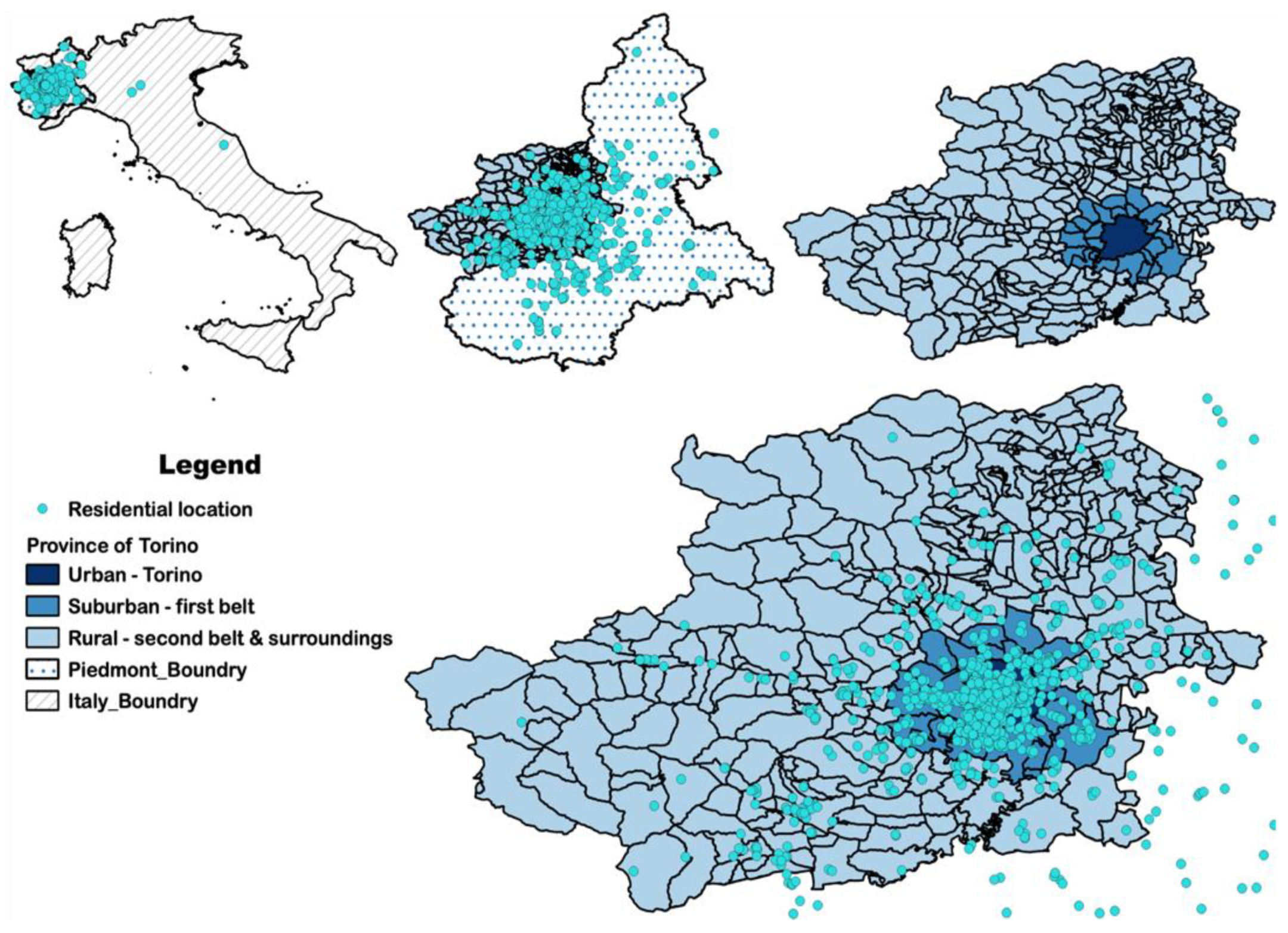
The research was conducted in the Piedmont region (Italy), with a focus on the metropolitan area of Torino. The Piedmont region, whose capital is Torino, is located in the north-west of Italy (Figure 1) and is bounded by Liguria to the south, by France to the west, by Valle d’Aosta and Switzerland to the north and by Lombardy and Emilia-Romagna to the east. The surface of the Piedmont region is around 25,400 square kilometres with 4,400,000 inhabitants (Source web-site of ISTAT Warehouse: http://dati-censimentopopolazione.istat.it/Index.aspx, accessed on 9 September 2020) (about 7.2% of the Italian population).

Figure 1. Urban, suburban, and rural division of study area with residential location distribution.

Most of the survey respondents live in Torino Province (Figure 1), which, in January 2015, was named the Metropolitan city of Torino (https://en.wikipedia.org/wiki/Province_of_Turin, accessed on 9 September 2020), covering an area of 6830 km² with a population of 2,306,676 (30 June 2011) and 316 municipalities—the highest figure in any province in Italy. Figure 1 shows the study area of Piedmont divided into urban, suburban, and rural areas, with the distribution of residential zones referring to the municipalities of the province of Torino.

A web questionnaire has been designed to obtain in-depth information related to the opinions, preferences, attitudes, lifestyles, and mobility patterns of users with the aim of studying the pro-environmental behaviour of the sample and understanding whether a general pro-environmental attitude may legitimately be assessed using the Rasch model. The four-step methodology comprised: (1) survey design; (2) survey administration and sample selection; (3) database construction; (4) model estimation and the testing of the GEB.

2.1. Survey Design

A survey has been designed, named “Come ci muoviamo? … ma soprattutto come vorremmo muoverci?” The survey is made up by two different web-questionnaires. The first part includes questions well established in the literature, ensuring well-grounded comparisons, and it is composed of six sections: mobility in a standard week; travel diary related to the most important trip; integrated mobility; mobility as a service; attitudes and preferences—including GEB; and socio-economic data. The second part incorporates new questions, derived from recent results of behavioural studies, to overcome some of the gaps observed in previous research by [18,19], and it is composed of two sections: information about the most important trip, and attitudes and preferences related to this trip. This paper mainly focuses on analysing general attitudes towards the environment and ecological behaviour using the section of the questionnaire related to GEB.

The GEB questionnaire is based on GEB-40 and GEB-51 but includes only the 26 items (GEB-26) reported in Table 1, resulting from deleting the redundant and problematic items found in GEB-40 and GEB-51. The questionnaire has been designed to collect polytomous data based on a 6-point Likert scale where 1 is “completely disagree” and 6 “completely agree”.

Table 1. Structure of GEB-26 questionnaire.

No.	Item Description	Code
	Category 1—Pro-social behaviour
1	Sometimes I give money to panhandlers	CS1
2	From time to time, I give money to charity	CS2
3	If an elderly or disabled person enters a crowded PT vehicle, I offer him/her my seat	CS3
4	If I were an employer, I would not hesitate to hire a person previously convicted of crime	CS4
5	Sometimes I ride public transport without paying a fare	CS6_REVC
	Category 2—Ecological garbage handling
6	I put dead batteries in the garbage	R1_REVC
7	I sort glass wastes for recycling	R5
	Category 3—Water and power saving
8	I turn off the heat at night	AE4
9	I wait until I have a full load before doing my laundry	AE5
10	In winter, I leave the windows wide open for long periods of time to let in fresh air	AE6_REVC
	Category 4—Ecologically aware consumerism
11	I use fabric softener with my laundry	CE1_REVC
12	I always look to buy vegetables from biological agriculture	CE6
13	Sometimes, I sell goods I don’t use anymore	CE7
14	Sometimes, I buy second-hand goods	CE8
15	Sometimes, I offer goods I don’t use anymore	CE9
16	Sometimes, I rent for free to someone, goods I occasionally use	CE14
17	I eat less meat than years ago	CE15
	Category 5—Garbage inhibition
18	I re-use plastic bag from the groceries	RR1
19	I sometimes buy beverage in cans	RR2_REVC
	Category 6—Environmental activism
20	I often talk with friends about problems related to the environment	V1
21	I am a member of an environmental organization	V2
22	In the past, I have pointed out to someone his or her un-ecological behaviour	V3
23	I sometimes contribute financially to environmental organizations	V4
24	I boycott companies using OGM or pesticides	V5
	Category 7—Transport
25	Usually, I do not drive my automobile in the city	T1
26	I usually drive on freeways at speeds lower than 100km/h	T2

Note: _REVC is added for items positively formulated as environmentally damaging and reverse coded.

2.2. Survey Administration and Sample Selection

The survey was administered to the residents in the Piedmont region, with focus on the metropolitan area of Torino. Citizens were reached through different channels: email, flyers, notices on the websites of municipalities and transport companies, formal notices to employees of Rail Infrastructure Managers, direct contact with major cultural and sport associations, newspapers, and local radio and Twitter, including the survey in the traffic bulletin. The link to the survey and QR code were available through the above channels and respondents completed the questionnaire using Computer-Assisted Web Interviewing (CAWI), developed through the software Lime Survey.

Such wide dissemination was possible thanks to the support from the local public bodies of the Piedmont Region, City of Torino, including the main universities (Politecnico di Torino and Università degli Studi di Torino), the transport authority Agenzia Mobilita Piemontese, and some transport operators, such as Gruppo Torinese Transporti and Sadem and the Rete Ferroviaria Italiana. Answers were collected in the period from the 27th of October 2017 to the 24th of April 2018, based on a snowball sampling plan, achieving a random sample of 4473 respondents.

2.3. Database Construction

The initial sample of 4473 records was resized to 4212 units excluding the persons whose destination was outside both Italy and the region. The 4212 records have been used in Rasch model estimation. The residential locations are classified into three areas, urban (metropolitan area of Torino), suburban (municipalities around Torino—first belt) and rural (rest of the territory—second belt). The Piedmont Territorial Demographic Observatory identifies the “first” and a “second” belts of municipalities surrounding Torino (https://web.archive.org/web/20140727134854/, http://www.demos.piemonte.it/site/images/stories/caricafile/territori/E_area_metropolitana.pdf, accessed on 15 July 2021). The majority of respondents came from urban areas, and the distribution of the three residential locations is: 2154 (51.14%) urban, 740 (17.57%) suburban, and 1318 (31.29%) rural (see Figure 1 for residential location distribution in urban, suburban and rural areas).

The next step for constructing the database was a check of missing values. Two variables, T1 and T2, related to category 7 “transport”, contained, respectively, 409 and 531 inapplicable responses. These were intentionally missed by respondents and were considered as missing during the analysis to avoid any imputation; we did, however, maintain a large database. The software Winsteps, used for the Rasch model, does not require complete data in order to provide estimates, because it uses Joint Maximum Likelihood Estimation (JMLE), which is very flexible as regards estimable data structures. Waterbury [34] reported that the Rasch model can handle varying amounts of missing data, provided that the missing responses are not missing at random. Hence, the missing records without any imputation were used, whereas other variables have complete data for the corresponding records. Finally, the dataset was transformed from the polytomous scale to the dichotomous scale by converting the first three categories, from 1 (completely disagree) to 3, to 1 “No”, and the next three categories, from 4 to 6 (completely agree), to 2 “Yes”.

2.4. Rasch Model as a Measure of General Ecological Behaviour

The general attitude towards the environment, based on the data collected by the GEB questionnaire, was analysed using the Rasch model for scale measurement. Rasch analysis describes procedures that use a particular model with outstanding mathematical properties developed by Georg Rasch [20] for the analysis of data from tests and questionnaires. The mathematical theory underlying Rasch models is a special case of Item Response Theory (IRT), and, more generally, a special case of a generalized linear model. The statistical calculations employed by the Rasch model to locate and rank persons and item difficulty are based on Guttmann Scaling and can be used with both dichotomous and polytomous datasets [35]. This study explores the potential of using the dichotomous Rasch model to analyse polytomous items for GEB attitude measurement.

The dichotomous Rasch model (DRM) [20] is the simplest model in the Rasch family. It was designed for use with ordinal data, which are scored in two categories. The DRM uses the summed scores from these ordinal responses to calculate interval-level estimates that represent person locations and item locations on a linear scale that represents the latent variable. The difference between person and item locations can be used to calculate the probability for a correct or positive response (x = 1), rather than an incorrect or negative response (x = 0). The equation for the DRM is as follows:

$$B_n-D_i=\ln \left(P_{ni}/1-P_{ni}\right)$$

(1)

where B_n = ability of a specific person n; D_i = difficulty of a specific item i; P_ni = probability of person n correctly answering item i; 1 − P_ni = probability of person n not correctly answering item i; and ln = “log-odds units” (logits), which is a natural logarithm.

The DRM specifies the probability, P, that the person n with ability B_n succeeds in item i of difficulty D_i.

The key Rasch model requirements are unidimensionality, local independence, person-invariant item estimates/person parameter separability, and item-invariant person estimates/item parameter separability.

For the parameter estimation of DRM, the Winsteps Rasch Analysis program version 4.8.0 was used. Winsteps implements two methods of estimating Rasch parameters from ordered qualitative observations: JMLE, also known as UCON (Unconditional Maximum Likelihood Estimation) [36], and PROX (Normal Approximation Algorithm) devised by Cohen [37].

Rasch Measures and Model Fit

The Rasch model fits are used to examine the unidimensionality of the latent trait to measure attitude towards GEB. Unidimensionality is evaluated using: (1) point–biserial correlation, (2) fit statistics, (3) Principal Component Analysis of Residuals, and (4) local independence.

Point–biserial Correlation. Point–biserial correlation is a useful diagnostic indicator of data miscoding or item mis-keying: negative or zero values indicate items or persons with response strings that contradict the variable. Li et al. [38] suggest that point-measure correlations larger than 0.3 indicate that items are measuring the same construct.

Fit Statistics. The Rasch model provides two indicators of misfit: INFIT and OUTFIT. INFIT (Inlier pattern-sensitive fit statistics) is sensitive to unexpected responses to items near the person’s ability level, and OUTFIT (outlier-sensitive fit statistics) considers differences between observed and expected responses regardless of how far away the item’s endorsability is from the person’s ability [39]. MNSQ (mean-square) is a Chi-square calculation for the OUTFIT and INFIT statistics. The ZSTD (Z-standardized) provides a t-test statistic measuring the probability of the MNSQ calculation occurring by chance. Since the ZSTD value is based on the MNSQ, as reported by Boone et al. [40], we first examine the MNSQ for evaluating fit. If the MNSQ value lies within an acceptable range, we ignore the ZSTD value. According to Boone et al. [40], INFIT and OUTFIT mean-square fit statistics between 0.5 and 1.5 represent productive items. For the mathematical formulation of point–biserial correlation, INFIT, OUTFIT, and ZSTD are derived from [18].

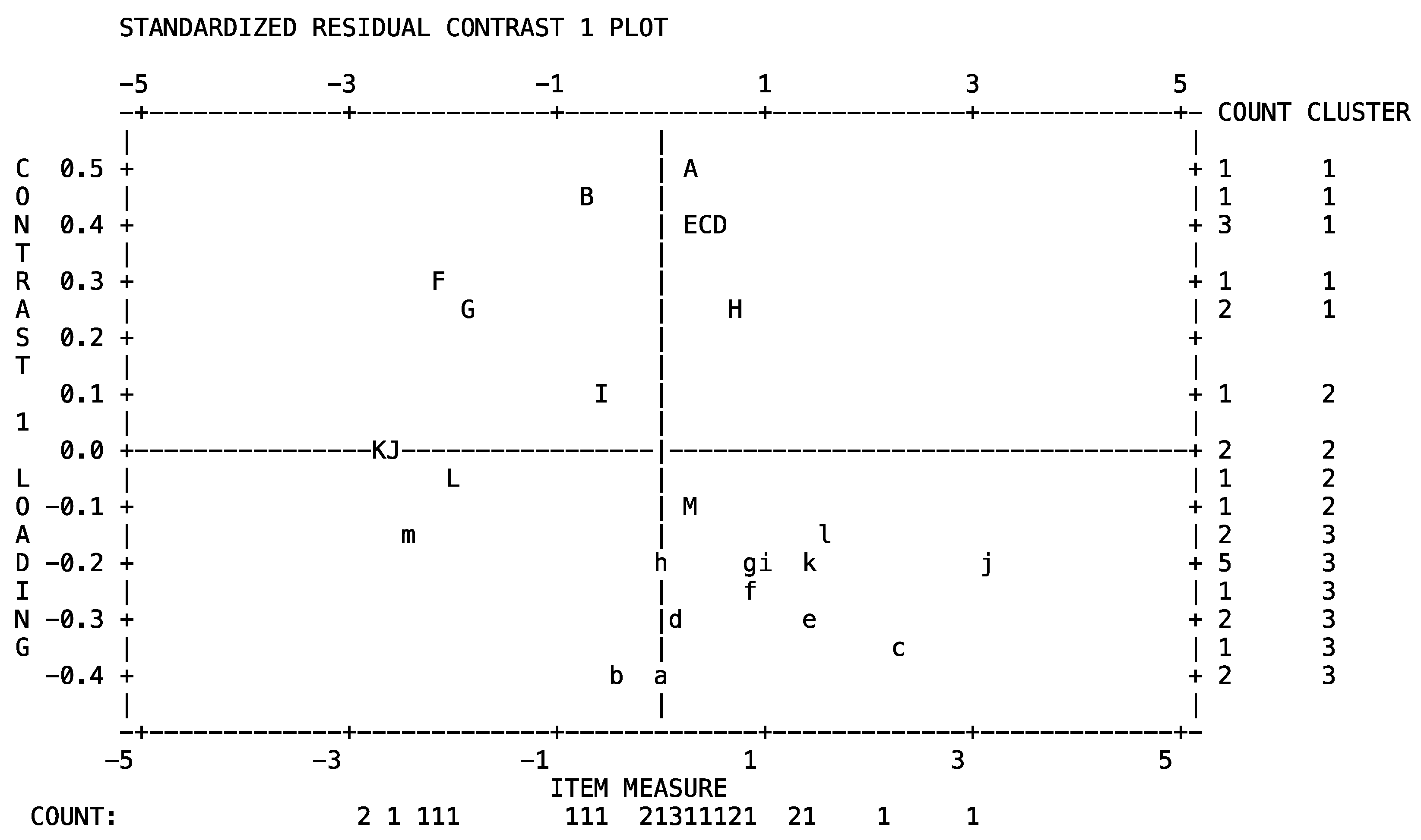
Principle Component Analysis of Residuals (PCAR). Unidimensionality was checked through PCAR. According to Reckase [41], unidimensionality pertains if: (a) the amount of variance explained by measures is >20%; (b) the unexplained variance of the eigenvalue for the first contrast is <3; and the unexplained variance accounted for by the first contrast is <5%.

Local Independence. Local independence means that after the contribution of the latent trait(s) to the data is removed, all that is left is random noise [42]. A correlation of r = 0.40 among items is low dependency.

Besides these, the Rasch model’s assumptions include assessing the reliability and separation of measures, differential item functioning, and the evaluation of item difficulty using Write map to evaluate construct validity.

Reliability and Separation index. This ranges from 0 to 1, and the higher the better [43]. Bond and Fox [44] suggested a value between 0.6 and 0.8 is acceptable. A separation index of 1.50 represents an acceptable level, 2 represent a good level according to Miller and Dishon [45], and 3 represents an excellent level as reported by Duncan et al. [46].

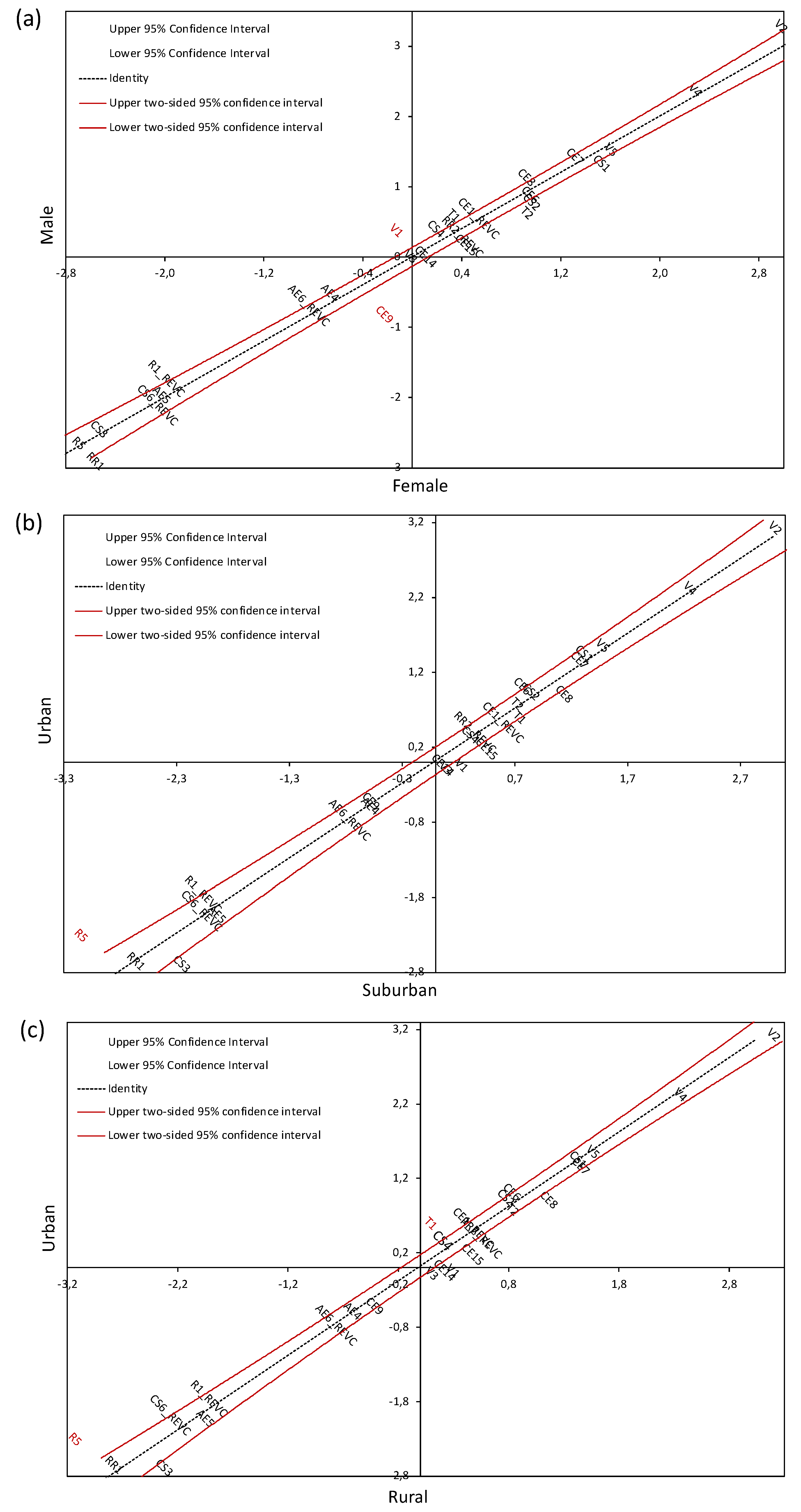
Differential Item Functioning (DIF). DIF is used to determine whether the individual items on a test function in the same way for two or more groups [47]. The Mantel–Haenszel (MH) [48] test for dichotomies is used. Items are flagged as DIF when the MH probability value is <=0.05 and then the DIF size is assessed according to the criteria set by Zwick et al. [49]. Moderate to large DIF pertains when the size of CUMLOR is ≥0.64, slight to moderate DIF pertains when the size of CUMLOR is ≥0.43, and DIF is negligible when the size of CUMLOR <0.43. We investigated DIF via two criteria: (1) gender and (2) residential location.

3. Results

The collected sample was composed of 2277 (50.91%) females, 2139 (47.82%) males, eight persons (0.18%) declaring to be part of another gender group, and 49 (1.09%) missing information. The average age of respondents was 36.43 years old (range from 12 to 96 years old), with 93.38% having a driving license. The majority of respondents (1909 individuals, 42.68%) are employees, followed by students (1851, 41.38%). In total, 30.83% of respondents live in a household composed of four persons. While 32.75% of households have two children, the majority (65.48%) have no children under 14 years old, and 17.86% did not answer this question. The income was classified into 13 levels, with the biggest group (17.46%) having a net income greater than EUR 10,000 per month. The second largest income group (12.77%) is the range of EUR 2501–3000/month (Table 2).

Table 2. Respondent’s socio-demographic characteristics (N = 4473).

Feature	Categories	Count	%
Gender	Male	2139	47.39
	Female	2277	50.91
	Other	8	0.18
	No answer	49	1.09
Age (years)	1–17	40	0.89
	18–25	1544	34.52
	26–40	1081	24.17
	41–60	1516	33.89
	60+	239	5.34
	No answer	53	1.18
Driving license	Yes	4177	93.38
	No	241	5.39
	No answer	55	1.23
Occupation	Looking for job	81	1.81
	Not occupied	24	0.54
	Pensioner	49	1.1
	Student	1851	41.38
	Homemade	5	0.11
	Worker	48	1.07
	Employee	1909	42.68
	Manager	79	1.77
	Teacher	177	3.96
	Self-employed	198	4.43
	Other	4	0.09
	No answer	48	1.07
Household composition	1	547	12.23
	2	947	21.17
	3	1154	25.8
	4	1379	30.83
	>4	393	8.79
	No answer	53	1.18
Children in household distribution	0	1402	31.34
	1	1170	26.16
	2	1465	32.75
	3	319	7.13
	>3	65	1.45
	No answer	52	1.16
Children under 14 in household distribution	0	2929	65.48
	1	488	10.91
	2	223	4.99
	3	33	0.74
	4	1	0.02
	No answer	799	17.86
Income distribution	1001–1500	506	11.31
	1501–2000	514	11.49
	2001–2500	512	11.45
	2501–3000	571	12.77
	3001–3500	451	10.08
	3501–4000	304	6.8
	4001–4500	250	5.59
	5001–6000	163	3.64
	6001–7000	66	1.48
	7001–8000	56	1.25
	8001–9000	35	0.78
	9001–10,000	28	0.63
	>10,000	781	17.46
	No answer	236	5.28

This section presents the results by following the various steps described in the methodology.

3.1. Point–Biserial Correlations

All items’ correlations are positive and point in the same direction. However, three small positive correlations are observed and analysed hereafter:

• Item AE6_REVC has a low correlation (0.05) close to zero. When assessing this item closely, 74.17% users agree, and 25.83% disagree, showing that this is one of the easiest behaviours to engage in (measure = −0.76);
• Item CS6_REVC has a low correlation (0.09) close to 0.1. When closely assessing this item, 90.38% users agree, and 9.62% disagree. Similar to the previous item, this is also one of the easiest behaviours to engage in (measure = −2.08). Most of the users stated using Public Transport (PT) without tickets, which may have caused the low correlation;
• Item CS4 has a low correlation (0.08) near to 0.1. When analysing this, no big differences among the addressed categories of the respondents (46.77% disagree and 53.23% agree) were found. This item seems to have a medium difficulty status across all respondents (Measure = 0.31).

3.2. Fit Statistics

Item AE6_REVC has the highest mean-square OUTFIT (1.55). The small difference of 0.05 over the threshold might not degrade the measurement. We found that all other items are within acceptable ranges of MNSQ, hence we are not investigating the ZSTD.

3.3. Principle Component Analysis of Residuals (PCAR)

First, the amount of variance explained by the measures is 34.2% (11.5% of raw variance explained by persons and 22.7% of raw variance explained by items), which is larger than the requirement of 20% according to Reckase [41]. Second, the unexplained variance by first contrast is 5.4%, which is slightly greater than 5%, but the eigenvalue of the first contrast is 2.14 (<3). The results suggest that the unidimensionality is consistent across the whole test.

The loadings of items on the first contrast of the residual-based PCA are shown in Figure 2, showing that this possible sub-dimension is formed from two items, A (AE6_REVC) and B (CS6_REVC). Items A and B have the largest loadings, quite far away from the general cluster created by the other items, and the eigenvalue of the first contrast is 2.14 (~2 items). To see the items corresponding to the letters of the alphabet represented in Figure 2, refer to Table 3.

Figure 2. Item loadings on the first contrast.

Table 3. Estimates of Item Parameters, INFIT, OUTFIT, and Point–Biserial Correlations.

Entry No.	Total Score	Measure	Model S.E.	INFIT		OUTFIT		Point–Biserial Correlation		Exact  Match (%)		Item
				MNSQ	ZSTD	MNSQ	ZSTD	CORR.	EXP.	OBS%	EXP%
10	7336	−0.76	0.04	1.24	9.90	1.55	9.90	A  0.05	0.33	70.9	75.7	AE6_REVC
5	8019	−2.08	0.05	1.10	2.54	1.48	6.48	B  0.09	0.24	90.4	90.4	CS6_REVC
4	6454	0.31	0.03	1.27	9.90	1.43	9.90	C  0.08	0.38	53.0	65.8	CS4
6	7938	−1.86	0.05	1.08	2.17	1.31	4.87	D  0.15	0.26	88.0	88.5	R1_REVC
19	6418	0.35	0.03	1.20	9.90	1.29	9.90	E  0.16	0.38	56.6	65.8	RR2_REVC
25	5712	0.46	0.04	1.15	9.90	1.24	9.90	F  0.20	0.37	58.6	65.5	T1
11	6248	0.53	0.03	1.14	9.90	1.22	9.90	G  0.23	0.38	59.8	65.8	CE1_REVC
26	5285	0.78	0.04	1.09	7.13	1.12	6.22	H  0.28	0.38	61.4	66.6	T2
8	7203	−0.58	0.04	0.99	−0.72	0.99	−0.26	I  0.35	0.34	73.9	73.3	AE4
13	5535	1.37	0.04	0.97	−1.91	0.95	−2.17	J  0.40	0.37	72.7	72.5	CE7
1	5491	1.43	0.04	0.96	−2.25	0.94	−2.33	K  0.41	0.37	74.1	73.1	CS1
14	5812	1.03	0.03	0.96	−3.36	0.93	−3.66	L  0.42	0.38	70.1	68.8	CE8
18	8185	−2.69	0.07	0.94	−1.15	0.87	−1.55	M  0.26	0.19	94.4	94.3	RR1
2	5949	0.87	0.03	0.93	−5.96	0.91	−5.22	m  0.45	0.38	70.8	67.5	CS2
7	8176	−2.64	0.07	0.93	−1.22	0.76	−2.93	l  0.27	0.20	94.1	94.1	R5
3	8136	−2.48	0.06	0.92	−1.62	0.76	−3.29	k  0.30	0.21	93.2	93.2	CS3
9	7985	−1.98	0.05	0.92	−2.03	0.85	−2.45	j  0.32	0.25	90.2	89.6	AE5
16	6673	0.06	0.03	0.91	−7.93	0.88	−7.00	i  0.47	0.37	70.6	66.8	CE14
17	6441	0.32	0.03	0.91	−8.75	0.86	−8.55	h  0.48	0.38	70.7	65.8	CE15
12	5911	0.92	0.03	0.90	−8.18	0.87	−7.59	g  0.48	0.38	72.5	67.8	CE6
21	4586	3.13	0.06	0.90	−2.48	0.72	−4.61	f  0.38	0.27	91.5	91.3	V2
22	6715	0.01	0.03	0.90	−8.58	0.87	−7.08	e  0.47	0.37	72.2	67.2	V3
15	7134	−0.49	0.04	0.89	−7.71	0.83	−6.86	d  0.47	0.35	76.3	72.2	CE9
20	6625	0.11	0.03	0.88	−9.90	0.83	−9.90	c  0.50	0.37	72.4	66.6	V1
24	5391	1.56	0.04	0.88	−6.88	0.83	−6.85	b  0.48	0.36	78.2	74.8	V5
23	4912	2.33	0.04	0.83	−6.48	0.66	−8.91	a  0.50	0.32	84.9	84.0	V4
Mean	6548.8	0.00	0.04	0.99	−1.0	1.00	−0.9	-	-	75.4	75.7	-
P.SD	1059.6	1.50	0.01	0.12	6.0	0.24	6.7	-	-	12.0	10.6	-

The correlations of the person measures computed with each cluster of items were as follows: cluster 1 and 2—r =1.0; cluster 1 and 3—r = 0.0587; cluster 2 and 3—r = 1.0. With clusters 1 and 3 having low correlation, the sub-dimension might be due to the items in cluster 1, as discussed above for items A and B. The detailed obtained correlation statistics are reported in Table A3 in Appendix A.

3.4. Local Independence

According to the Linacre guidelines (https://www.winsteps.com/winman/table23_99.htm, accessed on 10 September 2020), all the items’ correlations are <0.4, hence no item residuals are correlated, reflecting the local independence assumptions of Rasch analysis. The correlation among all variables is reported in Table A4 in Appendix A.

3.5. Reliability and Separation Index

The person measure reliability is 0.67 and item measure reliability is 1 (perfect), which is acceptable, with less of the variability of the measurement attributed to measurement error. The person separation, equal to 1.44, shows that this test can distinguish between high and low performers (1.44, ~2 levels) and represent a good level of separation according to Miller and Dishon [45]. The item separation is very high, equal to 34.22, and represents an excellent level of separation [46]. With this large person sample, the item difficulties are estimated very precisely, validating the GEB construct’s validity (>3).

3.6. Differential Item Functioning (DIF)

DIF is assessed using the MH test, based on gender (female, male) and residential location (urban, suburban, rural), and it is conducted by comparing a reference group (the majority group) with a focal group (the minority group) [50]. The reference groups for gender and for residential location are, respectively, female and urban, while the others are the focal groups.

Considering gender, two items report DIFs of slight to moderate sizes: CE9, with p value 0.00 and DIF size 0.63; and V1, with p value 0.00 and DIF Size −0.47. Looking at residential location, two items, R5 and T1, show moderate to large DIFs: R5, with p value 0.00 and DIF size 0.90 for urban and rural, and a p value 0.00 and DIF size 1.12 for urban and suburban. T1 has a p value 0.00 and DIF Size 0.44. The MH statistics for all variables are reported in Table A5 and Table A6 in Appendix A.

The item difficulty across two subgroups with item parameter estimates are plotted against each other in Figure 3, with a 95% confidence interval for both dimensions. The graph compares the reference and focal group item difficulties. The diagonal line represents the line along which all items would lie within a 95% confidence interval if there were no differences between subgroups. If the items fall within a range of 95% confidence interval, we can conclude that the items are homogenous across subgroups, that is, they have the same difficulty. The difficult items are highlighted in red across different subgroups in Figure 3.

Figure 3. Pair plot for DIF identification by (a) gender and (b,c) residential location.

Figure 3a shows that item CE9 (Sometimes, I offer goods I don’t use anymore) is more difficult for females; women seem not to agree to giving away items they use less as compared to men. Item V1 (I often talk with friends about problems related to the environment) is more difficult for males (Figure 3a); men seem to talk less often about environmental problems as compared to females. Item R5 (I sort glass wastes for recycling) in Figure 3b,c is more difficult for the urban population; the reason might be that differential garbage collection has not been enacted in all the subzones in urban areas as compared to suburban and rural areas. The reason for the higher difficulty for item T1 (Usually, I do not drive my automobile in the city) for the urban population refers to the frequent use of cars by people living in those areas, as they are perceived as much more comfortable than PT. People living in rural areas, connected through trains or suburban buses, prefer to avoid driving in big cities and congested areas. The difficult items are highlighted in red across different subgroups in Figure 3.

3.7. Write Map

Figure 4 depicts the person measures (left) and the item measures (right). Persons at the top experienced the least difficulty with engaging in the items, while persons at the very bottom had the most difficulty engaging in the items. We can observe that:

Figure 4. Write map.

• The most difficult item is V2, followed by item V4. Both belong to the category of environmental activism;
• The easiest items are R5 and RR1, followed by CS3. These three items are not addressed towards any individual person. Some persons above and below these items are less inclined towards GEB, so these items are not useful to the GEB measurement, but they still fall within the user’s ability range;
• Items CS1 and V5 measure similar portions of the trait, and therefore, from a measurement perspective, are redundant. This is also the case for items CE6, CS2 and T2, CE1_REVC and T1, CE15, CS4 and RR2_REVC, CE14 and V3, AE4 and CE9, AE5 and CS6_REVC, and R5 and RR1. Within groups of items, individual items can be removed, sacrificing a small degree of precision in the measurement;
• No gaps between items of more than a logit are evident, but there is a need to fill the measurement gaps between V4 and CS1 and between items AE6_REVC and R1_REVC. This explains the relatively poor value of the individual separation reliability.

4. Discussion

The purpose of this research was to scrutinize the psychometric properties of the GEB-26 questionnaire using a DRM approach to validate and to compare the scale with those used in previous research, and to understand whether this has some impact on travel behaviour, specifically on mode choice.

Unidimensionality has been evaluated utilizing Rasch fit statistics, as well as PCAR and point–biserial correlations. Notably, all these tests of the measure’s dimensionality suggest the items lie on one trait, as hypothesized during the survey design stage. Therefore, it can be recommended to use GEB-26 as a unidimensional scale. The model fit indicators suggest that the scale contains one particularly misfitting item, AE6_REVC, with only a slightly high outfit MNSQ value (0.05) that does not threaten the validity of the scale, such that we do not suggest deleting it. The fact that item AE6_REVC was the only item with poor fit demands further investigations, as it offers potential insights into the structure of GEB. It is well known that negatively coded items, especially if there are only a few and they are located at the end of the questionnaire, may be confusing for the respondents [51]. However, it is also possible that the item did not confuse the respondents, and that not behaving ecologically may not be seen as an inverse conceptualization of ecological behaviour, instead having a (partly) different construct in its own right. Moreover, local independence, reliability, and separation index assumptions were confirmed with good Rasch measure validity.

We have obtained the perfect level of reliability of 1, a separation of 34.22 for items, and a sufficient level of person separation and reliability. However, person (test) reliability mainly depends on the variance of sample ability, and on the number of categories per item. If we have more categories, then we might achieve higher person reliability. So, in this study, we first validated the questionnaire by converting the polytomous scale to the dichotomous scale to compare the results from the previous studies (GEB-40 and GEB-51), and to verify how the selected test performs with larger sample sizes, as person separation and reliability are also sample-dependent. The most important aspect is to validate the questionnaire’s items that have been selected, and to revise them, if necessary, for designing the next survey.

Observing the DIF analysis, it can be noticed that item CE9 is more difficult for females and V1 is more difficult for males. This shows that cultural, societal, and attitudinal differences are determinant factors of engaging in a certain behaviour. The DIF size for these two items was slight to moderate, hence we are not considering excluding these items for the next questionnaire. This aspect is also part of Campbell’s paradigm [52] of attitude, which states that some behaviours may be more difficult in certain contexts than in others. This applies also to the residential location (R5) and the related land use; the results show how a well-dispersed habit of sorting glass for recycling is easier for people living in rural areas due to the different organizational structure of collection points for glass at single homes, differently from the scattered patterns of collection points in cities. The way of life in rural areas also makes people less accustomed to driving in congested urban traffic (T1), which is why urban citizens are more used to, and thus inclined towards, using a car to travel inside the cities; differently, those living outside prefer traveling into the city by train or suburban bus to avoid traffic and parking problems. As such, the statement of Arnold et al. [15] holds true, showing the importance of surroundings and contextual elements in the daily routine. The DIF size for R5 is moderate to large, which must be considered in further analysis; on the other hand, item T1 has a slight to moderate DIF, not necessarily indicating it for deletion.

In the Write map, item RR1 (I re-use plastic bag from the groceries) can be identified as one of the easiest behaviours to perform in the GEB scale, showing it as a common habit of the studied population not only in Italy [18] but also in other countries, as reported in previous studies by Hergesell [22] in Germany and by Kaiser and Wilson [12] in Switzerland. Likewise, the item R5 (I sort glass wastes for recycling) is also found to be one of the easiest actions (with measure of −2.64) in both our and other studies [18,21]. Gaborieau and Pronello [18] reported the measure of this item (R5) to be equal to −3.35 (in GEB-40) in the Italian sample, −3.55 in the Swiss sample, and −2.44 in the Swedish sample. These findings reveal that this behaviour appears to be the easiest across all the samples.

Similarly, item V2 (I am a member of an environmental organization) and V4 (I sometimes contribute financially to environmental organizations) were the most difficult to endorse by both the respondents of this study (with measures of 3.13 and 2.33, respectively) and by those who answered the GEB-40 [18] (with measures of 3.31 and 2.21, respectively), showing similar measure of difficulty. The difficulty related to environmental activism items shows the low interest of Italian travellers in being a member of environmental organizations and financially contributing to them. The same item, V2, was also reported as one of the more difficult behaviours by Kaiser [33]. He measured ecological behaviour using the Rasch model in a study of 445 members of two Swiss transport associations: one aiming to promote a transport system with the smallest possible negative impact on human beings and nature, and the second primarily representing automobile drivers’ interests in 1998. The results show the consistency of this behaviour, which remained at the same level of difficulty even after decades. Gaborieau and Pronello [18] also reported on a comparison of Italian (GEB-40), Swiss and Swedish populations’ GEB. The GEB measures of Swiss and Swedish samples were taken from Kaiser and Biel [21]. They [18] reported that item V2 (with measure of 1.36 in Switzerland and 2.78 in Sweden) and item V4 (with measures of −0.35 in Switzerland and 1.87 in Sweden) are difficult among Italian travellers compared to Swiss and Swedish travellers, which is also confirmed by this study.

The second aspect that was investigated, concerning the validity of GEB in influencing the modal choice, is key in the current debate on climate change, which calls for major changes in people’s daily lifestyles [2]. A frequent question arising is as follows: do the actions people report to protect the environment reflect the environmental impacts they generate? If, theoretically speaking, this relation could hold true, under an empirical assessment our results show the opposite. We observed that out of the selected sample of 4212 respondents, for the most important trip (that with the longest distance), 1368 (32.48%) use a trip chain, followed by 1156 (27.45%) using a car, 729 (17.31%) using PT, 330 (7.83%) walking, and 310 (7.36%) cycling. Looking into trip chain, cars are used by the highest percentage of respondents, 1333 (31.65%), followed by 1096 people (26.02%) using PT, 667 traveling by train, 401 walking, and 322 cycling. This finding shows how people do not do what they intend to or say they will do. Hence, behavioural measures of ecological lifestyles may reflect the actual environmental impact in some other contexts, such as in electricity consumption, as reported by Arnold et al. [15], but they do not apply in the transport sector, as determined by looking at the results and as shown in previous studies [27,29,30,31,53]. This is referred to as the attitude–behaviour gap [54], or the behaviour–intention gap [55], demonstrating the volatility of the concepts of attitude or intention [56]. The results obtained in this research also contradict what was found in GEB-40 [18], where high GEB scores were attained by those users who use soft modes (walking or bike) for their most frequent trips, followed by PT (regional train, bus, tram, or metro) and then private motorized vehicles (car or motorbike). One reason for this contradiction might be that the trip chain was excluded by Gaborieau and Pronello [18], and their sample was smaller (108 users). This discrepancy will be further investigated in a continuation of the research. In Figure 5, the relation between the GEB Rasch measure and travel behaviour (mode choice) shows the discrepancy between mode choice and corresponding GEB (attitude–behaviour gap). In fact, while the highest GEB score refers to bike and bike sharing, the average GEB scores of PT users and those who walk are lower than those of cars, which was the first mode chosen by respondents after trip chain.

Figure 5. Box plot of the mean GEB score estimates for each travel mode.

It should also be recalled that the sample sizes in previous studies—in the Italian context (GEB-40 and GEB-51), in the Swedish and Swiss context [21], and in the Californian context [16]—were too small, although still within acceptable boundaries, according to Linacre [23]. Nevertheless, replication in a larger sample is highly desirable, as suggested in the current research. Regarding the generalizability of the results, it must be noted that the samples in previous studies were formed via a stratified sampling plan. Thus, different results may be observed when the sample follows the snowball sampling approach, and the participants are, as in this case, younger, and/or have a lower educational level. Finally, it needs to be emphasized that even excellent internal validity is no assurance that a given scale will also exert good external validity.

In fact, the effect of a larger sample size and the good selection of items in GEB-26 (by excluding problematic items identified in GEB-40 and GEB-51) generated a perfect level of reliability of 1, while during GEB-40 [18] and GEB-51 [19] analysis, the obtained item reliability values were, respectively, 0.96 and 0.94. Moreover, the total raw variance explained by the GEB-26 Rasch measures was 34.2%, which is higher than that of GEB-40 [18] at 31.6% (for GEB-51 raw variance by measures was not reported).

5. Conclusions

The final aim of the research is to assist policy makers in defining targeted policies to induce sustainable travel choices. To this end, measuring the efficacy of such policies—as, for example, environment-focused transport education, giving incentives when people use sustainable modes, or the adoption of technology to engage people in pro-environmental behaviour with the help of smartphone apps [57]—would help us to understand whether people are made aware of their environmental footprints, and are thus more motivated to behave in an ecological and sustainable manner.

The barriers to changing travel behaviour, such as the lack of ecological awareness, must be considered, resulting in different strategies for different typologies of travellers. Strategies cannot aim at changing the travellers, but should address the different groups, and focus on favouring the choice of environmentally-friend modes of transport, considering that behavioural changes can only be achieved via a major societal change.

A wider use of the effective GEB questionnaire (with attention paid to the inclusion of good items) by practitioners could make identifying good practices easier, helping them to come up with effective public policies and marketing campaigns. Moreover, the specific construction of a Rasch model for measurement purposes allows the development of adaptive surveys that can be used to make questionnaires shorter, selecting the items that matter, and matching with the abilities of different individuals.

We may conclude that GEB-26 shows acceptable approximation to the Rasch requirements and presents good psychometric properties when using DRM to validate the scale. Some further analyses may be useful to verify the three items (AE6_REVC, CS6_REVC and CS4) that are closer to the borderline, with low point–biserial correlations.

Further research is needed to deepen our understanding of the GEB and to devise appropriate measurement instruments. No evidence emerged that individuals with diverging sociodemographic characteristics, such as age, had different understandings of the items. Item that are difficult could be achieved by respondents with high capabilities, whilst easy items could be achieved by respondents with high and low abilities. Overlapping items measure different elements with different levels of difficulty [58], hence we do not suggest excluding items by looking only at their redundancy in the Write map when designing a new survey. Some recommendations deserve quoting for scale improvement. Firstly, more items could be selected with high or low difficulties, so that the scale will be more able to measure individuals outside of the intermediate level of ecological behaviour, helping to fill in the gaps identified in the study in the Write map analysis. This is important because the limited differentiation capabilities may attenuate the existing effects of measuring ecological behaviour. GEB-26 might not be capable of detecting strong effects potentially attributable to interventions based on ecological behaviour in terms of larger person ability range due to the weaknesses of the questionnaire’s design; in fact, we obtained a person measure reliability equal to 0.67 and person separation equal to 1.44, which values are acceptable but not excellent. Hence, GEB researchers would profit from more sensitive measurement instruments capable of detecting differences between individuals who are high and low in terms of ecological behaviour. Furthermore, we do not suggest excluding any item by looking only at the dichotomous scale measurement. Item exclusion will be further assessed after measuring the original six-scale polytomous questionnaire using the Rasch rating scale model, which is the next step of our research, whilst continuing to validate and select the most appropriate measurement scale to measure the GEB of users. As suggested by Linacre (https://www.winsteps.com/winman/reliability.htm, accessed on 10 September 2020), scales with more categories are expected to give better and higher person reliability and separation. Future research may also proceed by testing the GEB questionnaire in different cultural and territorial contexts, such as different regions, cities, and metropolitan areas of Italy, and different European countries, to validate the appropriate GEB questionnaire.

Improvements, as outlined above, are strongly recommended, and may provide a measurement tool that is reliable and internally valid for measuring GEB, thus allowing public bodies to measure the efficacy of adopted policies.

One of the limitations of studies assessing ecological and environmental behaviour is that people may not be aware about their environmental impacts and/or the damage they cause to the environment. As reported by Hamidi and Zhao [59], individuals who have greater environmental awareness are more likely to travel by PT or cycling if their physical conditions facilitate using these modes. Similarly, Matthies et al. [25] identified that women are more willing to reduce car use because of their stronger ecological norms and weaker car habits. The importance of habits holds true when considering environment-friendly consumer behaviour; as shown by Dahlstrand and Biel [60], the environmental concern (environmental values and a sense of responsibility for the environment) is more influential when habits are weak. Therefore, interventions based on the activation of norms related to general ecological behaviour have to be implemented at an early stage when travel habits are not yet well established (e.g., at the age from 14 to 16, or, at the latest, during driving school). Hence, proper environmental and mobility education is needed to educate people, as also suggested by Gaborieau and Pronello [18] and by Pronello and Camusso [53].