
Renewable Energy Consumption and Carbon Emissions—Testing Nonlinearity for Highly Carbon Emitting Countries


Abstract
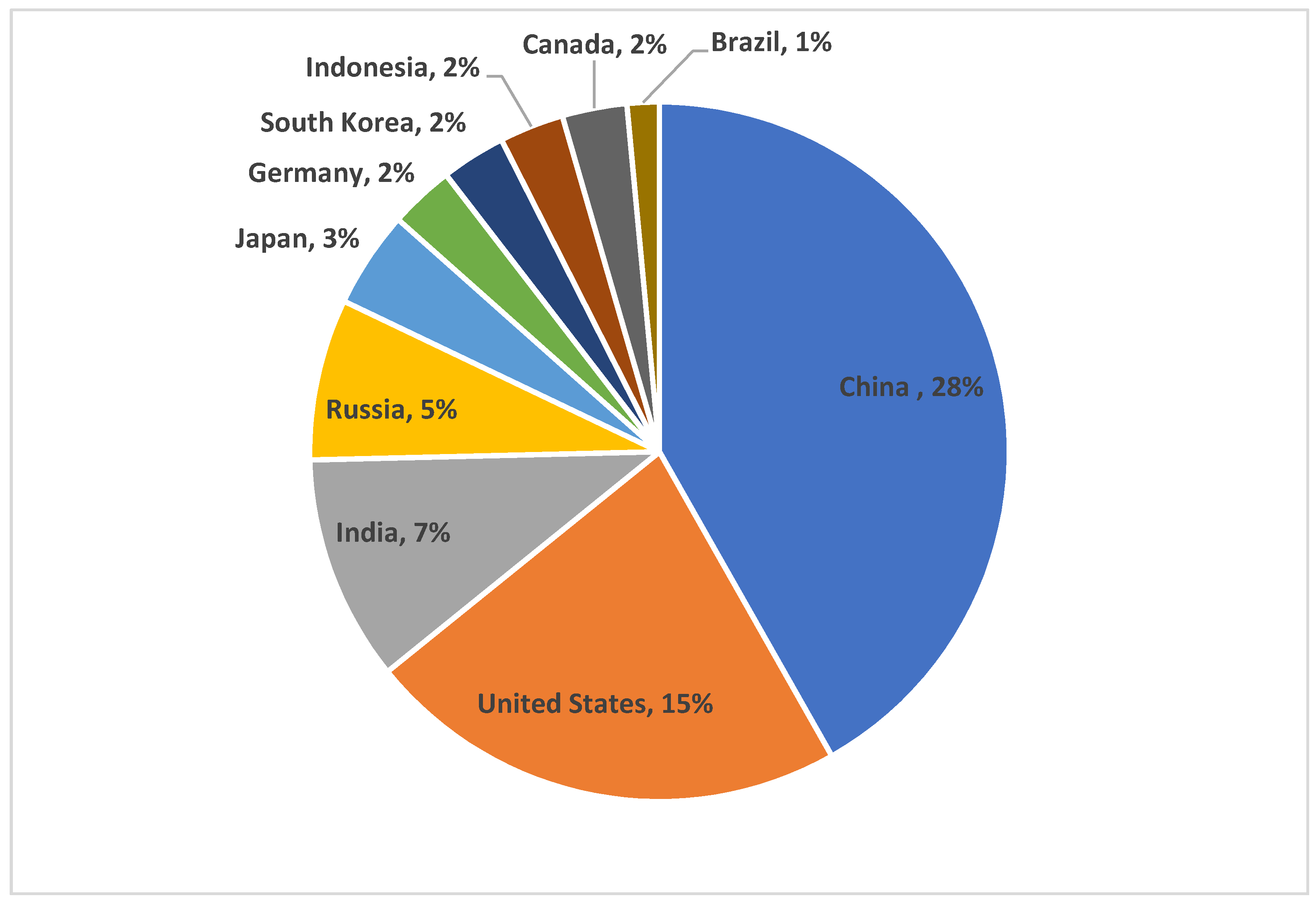
:1. Introduction
2. Literature Review
3. Empirical Model
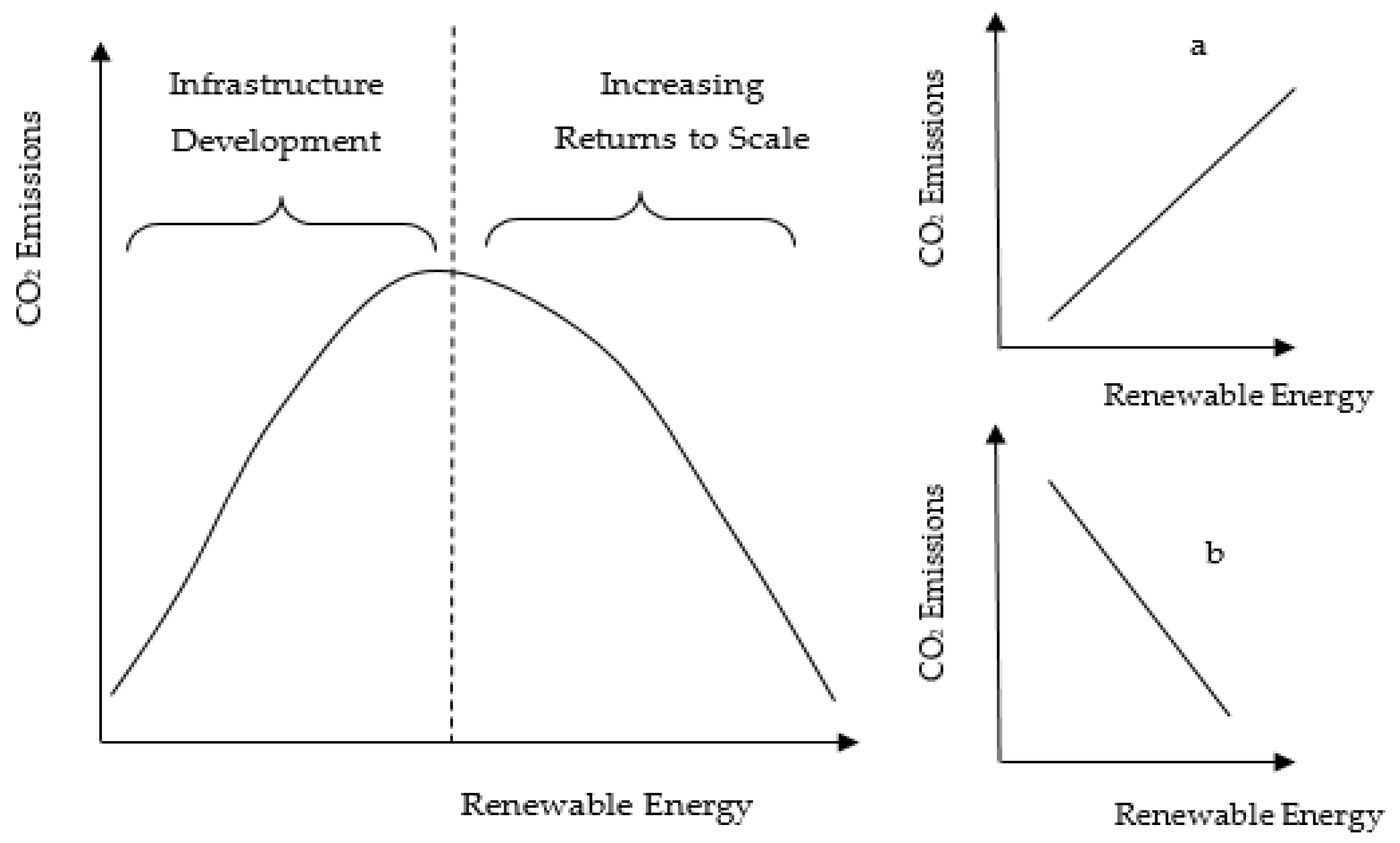
3.1. Theoretical Background
3.2. Modeling and Data
4. Procedural Outline
4.1. Panel Unit Root Test
4.2. Panel Cointegration Test
4.3. Panel ARDL/Pooled Mean Group
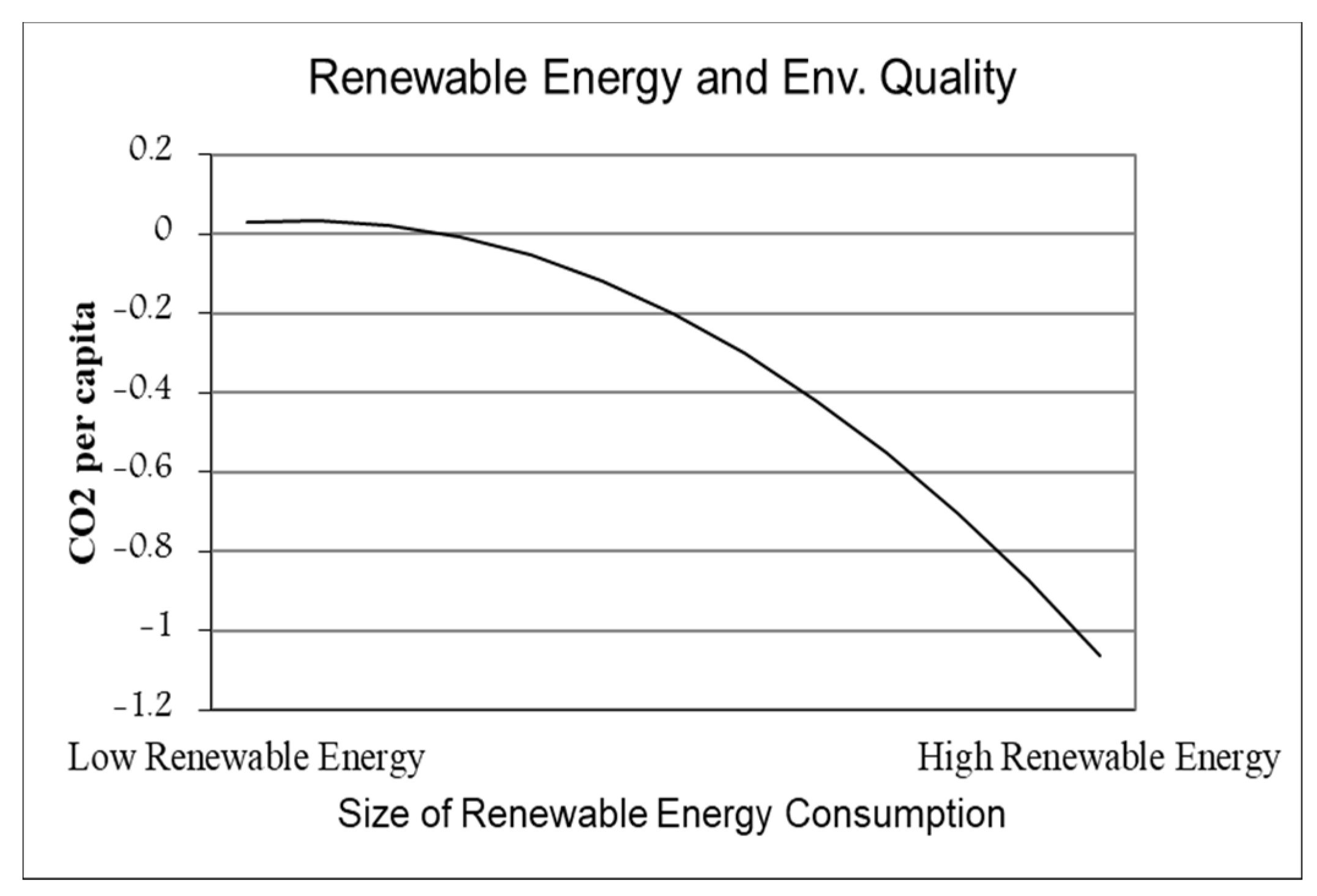
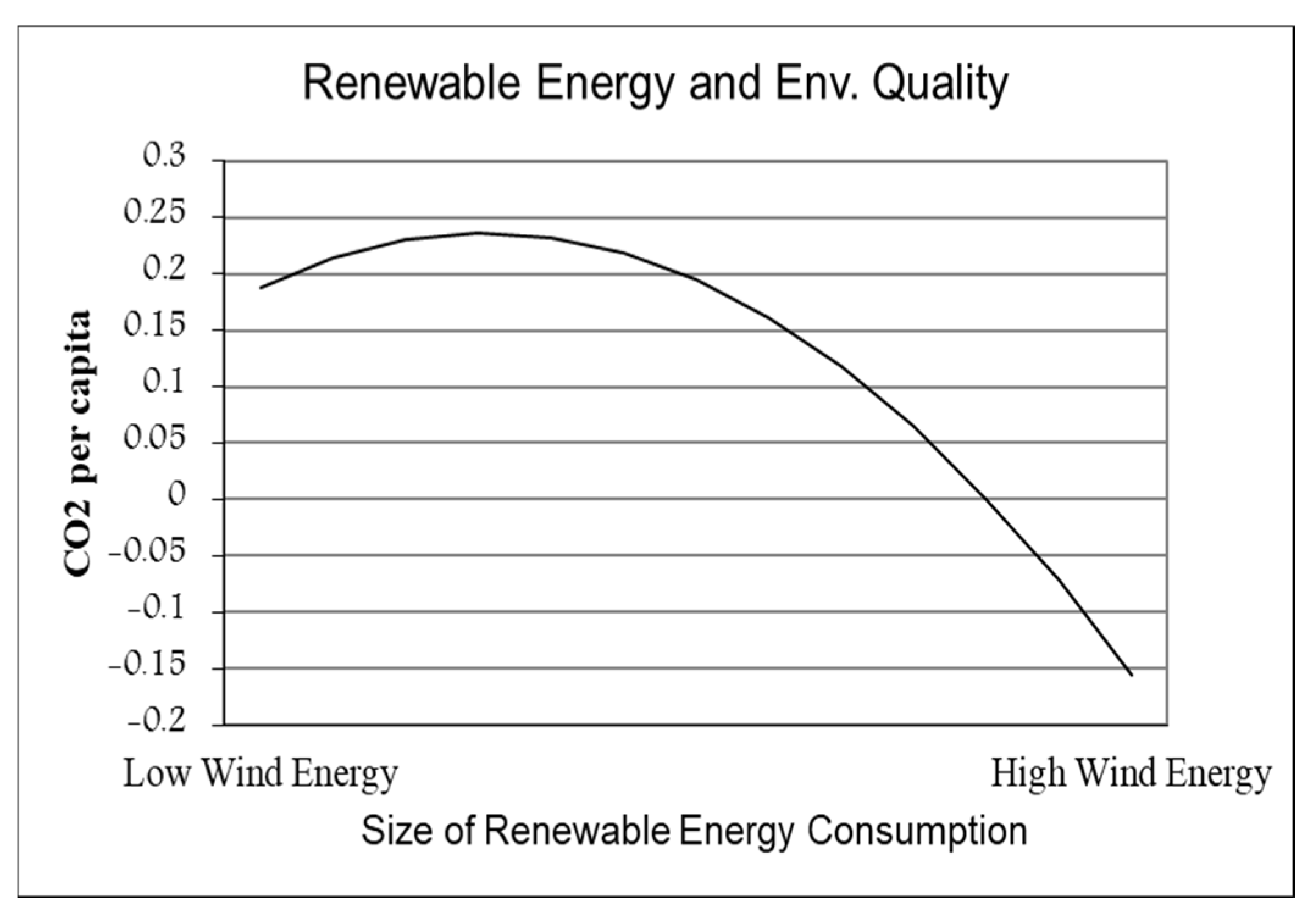
5. Analysis and Discussion of Results
Descriptive Statistics
6. Implications for Cleaner Production Based Development
7. Conclusions
Author Contributions
Funding
Institutional Review Board Statement
Informed Consent Statement
Data Availability Statement
Conflicts of Interest
References
- Thomas, S.; Rosenow, J. Drivers of increasing energy consumption in Europe and policy implications. Energy Policy 2020, 137, 111108. [Google Scholar] [CrossRef]
- Sinha, A.; Shahbaz, M.; Balsalobre, D. Exploring the relationship between energy usage segregation and environmental degradation in N-11 countries. J. Clean. Prod. 2017, 168, 1217–1229. [Google Scholar] [CrossRef] [Green Version]
- BP. Statistical Review of World Energy; British Petroleum: London, UK, 2019. [Google Scholar]
- Dong, K.; Dong, X.; Jiang, Q. How renewable energy consumption lower global CO2 emissions? Evidence from countries with different income levels. World Econ. 2020, 43, 1665–1698. [Google Scholar] [CrossRef]
- WDI. World Development Indicators; World Bank: Washington, DC, USA, 2019. [Google Scholar]
- NPR News Staff. What Countries Are Doing to Tackle Climate Change. Available online: https://www.npr.org/2011/12/07/143302823/what-countries-are-doing-to-tackle-climate-change (accessed on 20 October 2021).
- Balcilar, M.; Ozdemir, Z.A.; Ozdemir, H.; Shahbaz, M. The renewable energy consumption and growth in the G-7 countries: Evidence from historical decomposition method. Renew. Energy 2018, 126, 594–604. [Google Scholar] [CrossRef] [Green Version]
- Shahbaz, M.; Sinha, A. Environmental Kuznets curve for CO2 emissions: A literature survey. J. Econ. Stud. 2019, 46, 106–168. [Google Scholar] [CrossRef] [Green Version]
- Kang, J.; Yang, Y. Energy carbon emission structure and reduction potential focused on the supply-side and demand-side. PLoS ONE 2020, 15, e0239634. [Google Scholar] [CrossRef]
- Li, X.; Zhang, D.; Zhang, T.; Ji, Q.; Lucey, B. Awareness, energy consumption and pro-environmental choices of Chinese households. J. Clean. Prod. 2021, 279, 123734. [Google Scholar] [CrossRef]
- Zafar, M.W.; Shahbaz, M.; Sinha, A.; Sengupta, T.; Qin, Q. How renewable energy consumption contribute to environmental quality? The role of education in OECD countries. J. Clean. Prod. 2020, 268, 122149. [Google Scholar] [CrossRef]
- UCS. Each Country’s Share of CO2 Emissions; Union of Concerned Scientists: Cambridge, MA, USA, 2020. [Google Scholar]
- Wei, W.; Cai, W.; Guo, Y.; Bai, C.; Yang, L. Decoupling relationship between energy consumption and economic growth in China’s provinces from the perspective of resource security. Resour. Policy 2020, 68, 101693. [Google Scholar] [CrossRef]
- Voskamp, I.M.; Sutton, N.B.; Stremke, S.; Rijnaarts, H.H. A systematic review of factors influencing spatiotemporal variability in urban water and energy consumption. J. Clean. Prod. 2020, 256, 120310. [Google Scholar] [CrossRef]
- Tugcu, C.T.; Topcu, M. Total, renewable and non-renewable energy consumption and economic growth: Revisiting the issue with an asymmetric point of view. Energy 2018, 152, 64–74. [Google Scholar] [CrossRef]
- Adams, S.; Acheampong, A.O. Reducing carbon emissions: The role of renewable energy and democracy. J. Clean. Prod. 2019, 240, 118245. [Google Scholar] [CrossRef]
- Rauf, A.; Liu, X.; Amin, W.; Rehman, O.U.; Li, J.; Ahmad, F.; Bekun, F.V. Does sustainable growth, energy consumption and environment challenges matter for Belt and Road Initiative feat? A novel empirical investigation. J. Clean. Prod. 2020, 262, 121344. [Google Scholar] [CrossRef]
- Chen, C.; Pinar, M.; Stengos, T. Renewable energy consumption and economic growth nexus: Evidence from a threshold model. Energy Policy 2020, 139, 111295. [Google Scholar] [CrossRef]
- Dogan, E.; Altinoz, B.; Madaleno, M.; Taskin, D. The impact of renewable energy consumption to economic growth: A replication and extension of. Energy Econ. 2020, 90, 104866. [Google Scholar] [CrossRef]
- Ganda, F. The impact of innovation and technology investments on carbon emissions in selected organisation for economic Co-operation and development countries. J. Clean. Prod. 2019, 217, 469–483. [Google Scholar] [CrossRef]
- Krozer, Y. Life cycle costing for innovations in product chains. J. Clean. Prod. 2008, 16, 310–321. [Google Scholar] [CrossRef]
- Noussan, M.; Tagliapietra, S. The effect of digitalization in the energy consumption of passenger transport: An analysis of future scenarios for Europe. J. Clean. Prod. 2020, 258, 120926. [Google Scholar] [CrossRef]
- Lin, B.; Ge, J. Valued forest carbon sinks: How much emissions abatement costs could be reduced in China. J. Clean. Prod. 2019, 224, 455–464. [Google Scholar] [CrossRef]
- Xu, W.; He, H.S.; Hawbaker, T.J.; Zhu, Z.; Henne, P.D. Estimating burn severity and carbon emissions from a historic megafire in boreal forests of China. Sci. Total Environ. 2020, 716, 136534. [Google Scholar] [CrossRef] [PubMed]
- Arshed, N.; Munir, M.; Iqbal, M. Sustainability assessment using STIRPAT approach to environmental quality: An extended panel data analysis. Environ. Sci. Pollut. Res. 2021, 28, 18163–18175. [Google Scholar] [CrossRef] [PubMed]
- UCS. Environmental Impacts of Renewable Energy Technologies; Union of Concerned Scientists: Cambridge, MA, USA, 2013. [Google Scholar]
- Cotton, A. What Is the Carbon Payback Period for a Wind Turbine? Available online: NewScientist.com (accessed on 4 September 2019).
- Saidi, K.; Mbarek, M.B. Nuclear energy, renewable energy, CO2 emissions, and economic growth for nine developed countries: Evidence from panel Granger causality tests. Prog. Nucl. Energy 2016, 88, 364–374. [Google Scholar] [CrossRef]
- Dogan, E.; Seker, F. The influence of real output, renewable and non-renewable energy, trade and financial development on carbon emissions in the top renewable energy countries. Renew. Sustain. Energy Rev. 2016, 60, 1074–1085. [Google Scholar] [CrossRef]
- Bhat, J.A. Renewable and non-renewable energy consumption—impact on economic growth and CO2 emissions in five emerging market economies. Environ. Sci. Pollut. Res. 2018, 25, 35515–35530. [Google Scholar] [CrossRef] [PubMed]
- Jin, T.; Kim, J. What is better for mitigating carbon emissions–Renewable energy or nuclear energy? A panel data analysis. Renew. Sustain. Energy Rev. 2018, 91, 464–471. [Google Scholar] [CrossRef]
- Irandoust, M. The renewable energy-growth nexus with carbon emissions and technological innovation: Evidence from the Nordic countries. Ecol. Indic. 2016, 69, 118–125. [Google Scholar] [CrossRef]
- Sharif, A.; Raza, S.A.; Ozturk, I.; Afshan, S. The dynamic relationship of renewable and nonrenewable energy consumption with carbon emission: A global study with the application of heterogeneous panel estimations. Renew. Energy 2019, 133, 685–691. [Google Scholar] [CrossRef]
- Cheng, C.; Ren, X.; Wang, Z. The impact of renewable energy and innovation on carbon emission: An empirical analysis for OECD countries. Energy Procedia 2019, 158, 3506–3512. [Google Scholar] [CrossRef]
- Dogan, E.; Seker, F. Determinants of CO2 emissions in the European Union: The role of renewable and non-renewable energy. Renew. Energy 2016, 94, 429–439. [Google Scholar] [CrossRef]
- Liu, X.; Zhang, S.; Bae, J. The impact of renewable energy and agriculture on carbon dioxide emissions: Investigating the environmental Kuznets curve in four selected ASEAN countries. J. Clean. Prod. 2017, 164, 1239–1247. [Google Scholar] [CrossRef]
- Saudi, M.H.M. The role of renewable, non-renewable energy consumption and technology innovation in testing environmental Kuznets curve in Malaysia. Int. J. Energy Econ. Policy 2019, 9, 299–307. [Google Scholar]
- Nathaniel, S.P.; Iheonu, C.O. Carbon dioxide abatement in Africa: The role of renewable and non-renewable energy consumption. Sci. Total Environ. 2019, 679, 337–345. [Google Scholar] [CrossRef] [PubMed]
- Sun, Y.; Lu, Y.; Wang, T.; Ma, H.; He, G. Pattern of patent-based environmental technology innovation in China. Technol. Forecast. Soc. Chang. 2008, 75, 1032–1042. [Google Scholar] [CrossRef]
- Lin, B.; Wang, X. Carbon emissions from energy intensive industry in China: Evidence from the iron; steel industry. Renew. Sustain. Energy Rev. 2015, 47, 746–754. [Google Scholar] [CrossRef]
- Ali, W.; Abdullah, A.; Azam, M. Re-visiting the environmental Kuznets curve hypothesis for Malaysia: Fresh evidence from ARDL bounds testing approach. Renew. Sustain. Energy Rev. 2017, 77, 990–1000. [Google Scholar] [CrossRef]
- Santra, S. The effect of technological innovation on production-based energy and CO2 emission productivity: Evidence from BRICS countries. Afr. J. Sci. Technol. Innov. Dev. 2017, 9, 503–512. [Google Scholar] [CrossRef]
- Jin, L.; Duan, K.; Shi, C.; Ju, X. The impact of technological progress in the energy sector on carbon emissions: An empirical analysis from China. Int. J. Environ. Res. Public Health 2017, 14, 1505. [Google Scholar] [CrossRef] [Green Version]
- Chen, W.; Lei, Y. The impacts of renewable energy and technological innovation on environment-energy-growth nexus: New evidence from a panel quantile regression. Renew. Energy 2018, 123, 1–14. [Google Scholar] [CrossRef]
- Shahbaz, M.; Nasir, M.A.; Roubaud, D. Environmental degradation in France: The effects of FDI, financial development, and energy innovations. Energy Econ. 2018, 74, 843–857. [Google Scholar] [CrossRef] [Green Version]
- Mensah, C.N.; Long, X.; Dauda, L.; Boamah, K.B.; Salman, M. Innovation and CO2 emissions: The complimentary role of eco-patent and trademark in the OECD economies. Environ. Sci. Pollut. Res. 2019, 26, 22878–22891. [Google Scholar] [CrossRef]
- Ellis, E.A.; Montero, S.A.; Gómez, I.U.H.; Montero, J.A.R.; Ellis, P.W.; Rodríguez-Ward, D.; Reyes, P.B.; Putz, F.E. Reduced-impact logging practices reduce forest disturbance and carbon emissions in community managed forests on the Yucatán Peninsula, Mexico. For. Ecol. Manag. 2019, 437, 396–410. [Google Scholar] [CrossRef]
- Iqbal, M. Disaggregated GDP and Carbon Emissions—Testing Nonlinearity for Selected HDR Listed Countries; University of Management and Technology: Lahore, Pakistan, 2018. [Google Scholar]
- Ahmad, A.; Zhao, Y.; Shahbaz, M.; Bano, S.; Zhang, Z.; Wang, S.; Liu, Y. Carbon emissions, energy consumption and economic growth: An aggregate and disaggregate analysis of the Indian economy. Energy Policy 2016, 96, 131–143. [Google Scholar] [CrossRef]
- Esso, L.J.; Keho, Y. Energy consumption, economic growth and carbon emissions: Cointegration and causality evidence from selected African countries. Energy 2016, 114, 492–497. [Google Scholar] [CrossRef]
- Li, J.; Li, S. Energy investment, economic growth and carbon emissions in China—Empirical analysis based on spatial Durbin model. Energy Policy 2020, 140, 111425. [Google Scholar] [CrossRef]
- Saidi, K.; Omri, A. The impact of renewable energy on carbon emissions and economic growth in 15 major renewable energy-consuming countries. Environ. Res. 2020, 186, 109567. [Google Scholar] [CrossRef] [PubMed]
- Wang, Q.; Su, M.; Li, R. Toward to economic growth without emission growth: The role of urbanization and industrialization in China and India. J. Clean. Prod. 2018, 205, 499–511. [Google Scholar] [CrossRef]
- Wang, Q.; Su, M. The effects of urbanization and industrialization on decoupling economic growth from carbon emission–a case study of China. Sustain. Cities Soc. 2019, 51, 101758. [Google Scholar] [CrossRef]
- Wang, Q.; Wang, S. Decoupling economic growth from carbon emissions growth in the United States: The role of research and development. J. Clean. Prod. 2019, 234, 702–713. [Google Scholar] [CrossRef]
- Wang, Q.; Zhang, F. The effects of trade openness on decoupling carbon emissions from economic growth–evidence from 182 countries. J. Clean. Prod. 2021, 279, 123838. [Google Scholar] [CrossRef]
- Yeh, J.-C.; Liao, C.-H. Impact of population and economic growth on carbon emissions in Taiwan using an analytic tool STIRPAT. Sustain. Environ. Res. 2017, 27, 41–48. [Google Scholar] [CrossRef] [Green Version]
- Hanif, N.; Arshed, N.; Aziz, O. On interaction of the energy: Human capital Kuznets curve? A case for technology innovation. Environ. Dev. Sustain. 2020, 22, 7559–7586. [Google Scholar] [CrossRef]
- Zahid, T.; Arshed, N.; Munir, M.; Hameed, K. Role of energy consumption preferences on human development: A study of SAARC region. Econ. Chang. Restruct. 2021, 54, 121–144. [Google Scholar] [CrossRef]
- Haans, R.F.; Pieters, C.; He, Z.-L. Thinking about U: Theorizing and testing U-and inverted U-shaped relationships in strategy research. Strateg. Manag. J. 2016, 37, 1177–1195. [Google Scholar] [CrossRef]
- Chiang, A.C.; Wainwright, K. Fundamental Methods of Mathematical Economics; McGraw-Hill Irwin: New York, NY, USA, 2005. [Google Scholar]
- Levin, A.; Lin, C.-F.; Chu, C.-S.J. Unit root tests in panel data: Asymptotic and finite-sample properties. J. Econ. 2002, 108, 1–24. [Google Scholar] [CrossRef]
- Kao, C. Spurious regression and residual-based tests for cointegration in panel data. J. Econ. 1999, 90, 1–44. [Google Scholar] [CrossRef]
- Pedroni, P. Panel cointegration: Asymptotic and finite sample properties of pooled time series tests with an application to the PPP hypothesis. Econ. Theory 2004, 20, 597–625. [Google Scholar] [CrossRef] [Green Version]
- Anwar, A.; Sinha, A.; Sharif, A.; Siddique, M.; Irshad, S.; Anwar, W.; Malik, S. The nexus between urbanization, renewable energy consumption, financial development and CO2 emissions: Evidence from selected Asian countries. Environ. Dev. Sustain. 2021, 1–21. [Google Scholar]
- Pesaran, M.H.; Shin, Y.; Smith, R.P. Pooled Mean Group Estimation of Dynamic Heterogeneous Panels. J. Am. Stat. Assoc. 1999, 94, 621–634. [Google Scholar] [CrossRef]
- Dong, K.; Dong, X.; Dong, C. Determinants of the global and regional CO2 emissions: What causes what and where? Appl. Econ. 2019, 51, 5031–5044. [Google Scholar] [CrossRef]
- Iqbal, M.; Kalim, R.; Arshed, N. Domestic and foreign incomes and trade balance-a case of south Asian economies. Asian Dev. Policy Rev. 2019, 7, 355–368. [Google Scholar] [CrossRef] [Green Version]
- Li, T.; Wang, Y.; Zhao, D. Environmental Kuznets curve in China: New evidence from dynamic panel analysis. Energy Policy 2016, 91, 138–147. [Google Scholar] [CrossRef]
- Shaari, M.S.; Abdul Karim, Z.; Zainol Abidin, N. The effects of energy consumption and national output on CO2 emissions: New evidence from OIC countries using a Panel ARDL analysis. Sustainability 2020, 12, 3312. [Google Scholar] [CrossRef] [Green Version]
- Xing, T.; Jiang, Q.; Ma, X. To facilitate or curb? The role of financial development in China’s carbon emissions reduction process: A novel approach. Int. J. Environ. Res. Public Health 2017, 14, 1222. [Google Scholar] [CrossRef]
- Enders, W. Applied Econometric Time Series, 4th ed.; Wiley: Hoboken, NJ, USA, 2014. [Google Scholar]
- Hassan, M.S.; Kalim, R. Stock market and banking sector: Are they complement for economic growth in low human developed economy? Pak. Econ. Soc. Rev. 2017, 55, 1–30. [Google Scholar]
- Arshed, N.; Zahid, A. Panel Monetary Model and Determination of Multilateral Exchange Rate with Major Trading Partners. Int. J. Recent Sci. Res. 2016, 7, 10551–10560. [Google Scholar]
- Dawson, J.F. Moderation in management research: What, why, when and how. J. Bus. Psychol. 2014, 29, 1–19. [Google Scholar] [CrossRef]
- Bulut, U. Testing environmental Kuznets curve for the USA under a regime shift: The role of renewable energy. Environ. Sci. Pollut. Res. 2019, 26, 14562–14569. [Google Scholar] [CrossRef]
- Acheampong, A.O.; Adams, S.; Boateng, E. Do globalization and renewable energy contribute to carbon emissions mitigation in Sub-Saharan Africa? Sci. Total Environ. 2019, 677, 436–446. [Google Scholar] [CrossRef]
- Vural, G. How do output, trade, renewable energy and non-renewable energy impact carbon emissions in selected Sub-Saharan African Countries? Resour. Policy 2020, 69, 101840. [Google Scholar] [CrossRef]
- Li, P.; Ouyang, Y.; Zhang, L. The nonlinear impact of renewable energy on CO2 emissions: Empirical evidence across regions in China. Appl. Econ. Lett. 2020, 27, 1150–1155. [Google Scholar] [CrossRef]
- Shahsavari, A.; Akbari, M. Potential of solar energy in developing countries for reducing energy-related emissions. Renew. Sustain. Energy Rev. 2018, 90, 275–291. [Google Scholar] [CrossRef]
- Zhang, M.; Anaba, O.A.; Ma, Z.; Li, M.; Asunka, B.A.; Hu, W. En route to attaining a clean sustainable ecosystem: A nexus between solar energy technology, economic expansion and carbon emissions in China. Environ. Sci. Pollut. Res. 2020, 27, 18602–18614. [Google Scholar] [CrossRef] [PubMed]
- Forbes, K.F.; Zampelli, E.M. Wind energy, the price of carbon allowances, and CO2 emissions: Evidence from Ireland. Energy Policy 2019, 133, 110871. [Google Scholar] [CrossRef]
- Kaldellis, J.K.; Apostolou, D. Life cycle energy and carbon footprint of offshore wind energy. Comparison with onshore counterpart. Renew. Energy 2017, 108, 72–84. [Google Scholar] [CrossRef]
- Karnauskas, K.B.; Lundquist, J.K.; Zhang, L. Southward shift of the global wind energy resource under high carbon dioxide emissions. Nat. Geosci. 2018, 11, 38–43. [Google Scholar] [CrossRef]
- Martin, C. Wind Turbine Blades Can’t Be Recycled, So They’ve Pilling Up in Landfills. Bloomberg Green, 5 February 2020. [Google Scholar]
- Tubiello, F.N.; Conchedda, G.; Wanner, N.; Federici, S.; Rossi, S.; Grassi, G. Carbon emissions and removals from forests: New estimates, 1990–2020. Earth Syst. Sci. Data 2021, 13, 1681–1691. [Google Scholar] [CrossRef]
- Khan, M.K.; Khan, M.I.; Rehan, M. The relationship between energy consumption, economic growth and carbon dioxide emissions in Pakistan. Financ. Innov. 2020, 6, 1–13. [Google Scholar] [CrossRef] [Green Version]
- Saint Akadiri, S.; Alola, A.A.; Olasehinde-Williams, G.; Etokakpan, M.U. The role of electricity consumption, globalization and economic growth in carbon dioxide emissions and its implications for environmental sustainability targets. Sci. Total Environ. 2020, 708, 134653. [Google Scholar] [CrossRef]
- Schröder, E.; Storm, S. Economic Growth and Carbon Emissions: The Road to “Hothouse Earth” is Paved with Good Intentions. Int. J. Polit. Econ. 2020, 49, 153–173. [Google Scholar] [CrossRef]


| Variables | Mean | S.D | Minimum | Maximum | Observations |
|---|---|---|---|---|---|
| ENV | 1.739 | 1.014 | −0.33 | 3.01 | 280 |
| REC | 2.365 | 1.306 | −0.817 | 4.057 | 250 |
| WEC | −3.17 | 3.156 | −11.5 | 2.09 | 241 |
| SEC | −4.86 | 2.985 | −10.8 | 1.289 | 217 |
| HEC | 1.403 | 1.26 | −1.76 | 3.641 | 280 |
| INN | 0.094 | 0.116 | 0.000 | 0.420 | 280 |
| FAS | 2.054 | 3.445 | 0.009 | 12.420 | 260 |
| ECG | 9.335 | 1.348 | 6.355 | 10.907 | 280 |
| Country | Renewable Energy Consumption | Wind Energy | Solar Energy | Hydro Energy |
|---|---|---|---|---|
| Brazil | 34.80181 | 3.84059 | 0.24852 | 30.7127 |
| Canada | 22.80599 | 1.73458 | 0.19121 | 20.8802 |
| China | 12.14472 | 2.5459 | 1.23469 | 8.36413 |
| Germany | 12.65646 | 8.08647 | 3.34532 | 1.22467 |
| India | 6.50715 | 1.70106 | 0.8668 | 3.93929 |
| Indonesia | 2.06452 | 0.02458 | 0.00228 | 2.03766 |
| Japan | 8.08133 | 0.34406 | 3.63278 | 4.10449 |
| Russia | 5.99758 | 0.00715 | 0.01793 | 5.9725 |
| South Korea | 1.11153 | 0.18208 | 0.70824 | 0.22121 |
| USA | 5.10868 | 2.13823 | 0.74771 | 2.22274 |
| At Level | At First Difference | |||
|---|---|---|---|---|
| Variables | Unadjusted T-Test | Adjusted T-Test | Unadjusted T-Test | Adjusted T-Test |
| ENV | −1.932 | −0.417 | −7.869 | −1.944 ** |
| REC | −2.199 | −0.589 | −8.473 | −2.015 ** |
| WEC | 5.691 | 11.313 | −8.828 | −1.517 * |
| SEC | −0.719 | 9.299 | −4.393 | −4.268 *** |
| HEC | −5.577 | −2.019 * | −14.603 | −7.989 *** |
| INN | −1.875 | 0.595 | −9.988 | −3.107 *** |
| FAS | −4.674 | −2.654 *** | −3.448 | −1.685 ** |
| ECG | −1.223 | −0.652 | −7.915 | −2.570 *** |
| Model 1 | Model 2 | Model 3 | Model 4 | |
|---|---|---|---|---|
| Pedroni Test | Test Statistic | Test Statistic | Test Statistic | Test Statistic |
| Modified Phillips-Perron t-test | 1.510 * | 1.133 | 2.483 *** | 1.989 ** |
| Phillips-Perron t-test | −3.150 *** | −1.573 * | −3.285 *** | −2.037 ** |
| Augmented Dicky-Fuller t-test | −3.664 *** | −2.551 *** | −2.716 *** | −2.432 ** |
| Westerlund Test | ||||
| Variance Ratio | −1.485 * | −1.953 ** | 0.215 | −0.876 |
| Variables | Dependent Variable: ENV | |||||||
|---|---|---|---|---|---|---|---|---|
| Model 1 | Model 2 | Model 3 | Model 4 | |||||
| Coeff. | S.E | Coeff. | S.E | Coeff. | S.E | Coeff. | S.E | |
| REC | 0.109 * | 0.061 | ||||||
| REC2 | −0.082 *** | 0.016 | ||||||
| WEC | −0.087 *** | 0.031 | ||||||
| WEC2 | −0.008 *** | 0.003 | ||||||
| SEC | −0.069 *** | 0.022 | ||||||
| SEC2 | −0.007 ** | 0.003 | ||||||
| HEC | −0.497 ** | 0.248 | ||||||
| HEC2 | 0.095 | 0.086 | ||||||
| INN | 0.183 | 0.177 | −0.923 | 0.698 | −0.942 ** | 0.458 | −3.206 *** | 1.188 |
| FAS | 0.139 *** | 0.031 | 0.103 | 0.093 | 0.178 ** | 0.075 | 0.174 | 0.122 |
| ECG | 0.568 ** | 0.039 | 0.890 *** | 0.117 | 0.727 *** | 0.092 | 0.656 *** | 0.109 |
| obs | 240 | 240 | 240 | 240 | ||||
| Cut off values | 0.66 | − | − | − | ||||
| Antilog. | 3.86% | |||||||
| Variables | Dependent Variable: ENV | |||||||
|---|---|---|---|---|---|---|---|---|
| Model 1 | Model 2 | Model 3 | Model 4 | |||||
| Coeff. | S.E | Coeff. | S.E | Coeff. | S.E | Coeff. | S.E | |
| ECMt-1 | −0.340 *** | 0.102 | −0.097 *** | 0.001 | −0.141 *** | 0.032 | −0.074 ** | 0.019 |
| ∆REC | 7.113 | 6.234 | ||||||
| ∆REC2 | −1.119 | 0.979 | ||||||
| ∆WEC | −0.018 | 0.127 | ||||||
| ∆WEC2 | −0.001 | 0.001 | ||||||
| ∆SEC | −0.027 | 0.187 | ||||||
| ∆SEC2 | −0.002 | 0.001 | ||||||
| ∆HEC | −0.017 | 0.017 | ||||||
| ∆HEC2 | −0.023 ** | 0.007 | ||||||
| ∆INN | 0.502 *** | 0.165 | 0.403 | 0.271 | 0.097 | 0.253 | 0.933 *** | 0.245 |
| ∆FAS | −1.601 | 12.837 | 0.202 | 0.351 | 0.079 | 0.886 | 0.042 | 0.318 |
| ∆ECG | 0.552 *** | 0.160 | 0.892 *** | 0.095 | 1.027 *** | 0.120 | 0.447 *** | 0.073 |
| Cons. | −1.215 *** | 0.336 | −0.676 *** | 0.198 | −0.762 *** | 0.213 | −0.306 *** | 0.112 |
| Conv. Speed | 2.94 | 10.31 | 7.09 | 13.51 | ||||
| Country | Effect of Renewable Energy | Effect of Wind Energy | Effect of Solar Energy | Effect of Hydro Energy |
|---|---|---|---|---|
| Brazil | −0.65 | −0.13 | 0.08 * | −1.70 |
| Canada | −0.46 | −0.05 | 0.09 * | −1.51 |
| China | −0.24 | −0.09 | −0.01 | −1.06 |
| Germany | −0.25 | −0.22 | −0.09 | −0.10 |
| India | −0.08 | −0.05 | 0.01 * | −0.68 |
| Indonesia | 0.04 * | 0.21 * | 0.16 * | −0.35 |
| Japan | −0.13 | 0.08 | −0.10 | −0.70 |
| Russia | −0.07 | 0.23 * | 0.16 * | −0.89 |
| South Korea | 0.01 * | 0.12 * | 0.02 * | 0.75 * |
| USA | −0.04 | −0.07 | 0.02 * | −0.40 |
Publisher’s Note: MDPI stays neutral with regard to jurisdictional claims in published maps and institutional affiliations. |
© 2021 by the authors. Licensee MDPI, Basel, Switzerland. This article is an open access article distributed under the terms and conditions of the Creative Commons Attribution (CC BY) license (https://creativecommons.org/licenses/by/4.0/).
Share and Cite
Salem, S.; Arshed, N.; Anwar, A.; Iqbal, M.; Sattar, N. Renewable Energy Consumption and Carbon Emissions—Testing Nonlinearity for Highly Carbon Emitting Countries. Sustainability 2021, 13, 11930. https://doi.org/10.3390/su132111930
Salem S, Arshed N, Anwar A, Iqbal M, Sattar N. Renewable Energy Consumption and Carbon Emissions—Testing Nonlinearity for Highly Carbon Emitting Countries. Sustainability. 2021; 13(21):11930. https://doi.org/10.3390/su132111930
Chicago/Turabian StyleSalem, Sultan, Noman Arshed, Ahsan Anwar, Mubasher Iqbal, and Nyla Sattar. 2021. "Renewable Energy Consumption and Carbon Emissions—Testing Nonlinearity for Highly Carbon Emitting Countries" Sustainability 13, no. 21: 11930. https://doi.org/10.3390/su132111930
APA StyleSalem, S., Arshed, N., Anwar, A., Iqbal, M., & Sattar, N. (2021). Renewable Energy Consumption and Carbon Emissions—Testing Nonlinearity for Highly Carbon Emitting Countries. Sustainability, 13(21), 11930. https://doi.org/10.3390/su132111930