Dynamic Electric Dispatch for Wind Power Plants: A New Automatic Controller System Using Evolutionary Algorithms

Abstract

In this paper, we use an evolutionary swarm intelligence approach to build an automatic electric dispatch controller for an offshore wind power plant (WPP). The optimal power flow (OPF) problem for this WPP is solved by the Canonical Differential Evolutionary Particle Swarm Optimization algorithm (C-DEEPSO). In this paper, C-DEEPSO works as a control system for reactive sources in energy production. The control operation takes place in a daily energy dispatch, scheduled into 15 min intervals and resulting in 96 operating test scenarios. As the nature of the optimization problem is dynamic, a fine-tuning of the initialization parameters of the optimization algorithm is performed at each dispatch interval. Therefore, a version of the C-DEEPSO algorithm has been built to automatically learn the best set of initialization parameters for each scenario. For this, we have coupled C-DEEPSO with the irace tool (an extension of the iterated F-race (I/F-Race)) by using inferential statistic techniques. The experiments carried out showed that the methodology employed here is robust and able to tackle this OPF-like modeling. Moreover, the methodology works as an automatic control system for a dynamic schedule operation.

1. Introduction

To meet the ambitious goals of the Paris agreement [1] to prevent, or at least minimize, climate change, there is a global need for sustainable energy supply. Part of this energy supply must be produced by renewable sources. Market-driven policies are increasingly focused on promoting the use of wind and solar generation [2]. The production of energy and electricity from wind sources can be carried out both on the ground (onshore) and in wind farms installed in the ocean (offshore). Locations for the construction of offshore wind power plants (WPPs) are usually a few hundred kilometers away from the nearest coast, which requires long-distance cables in the ocean [3]. Being quick to install, especially when compared to other energy sources, great efforts to develop onshore and offshore wind farms are being made [4,5]. 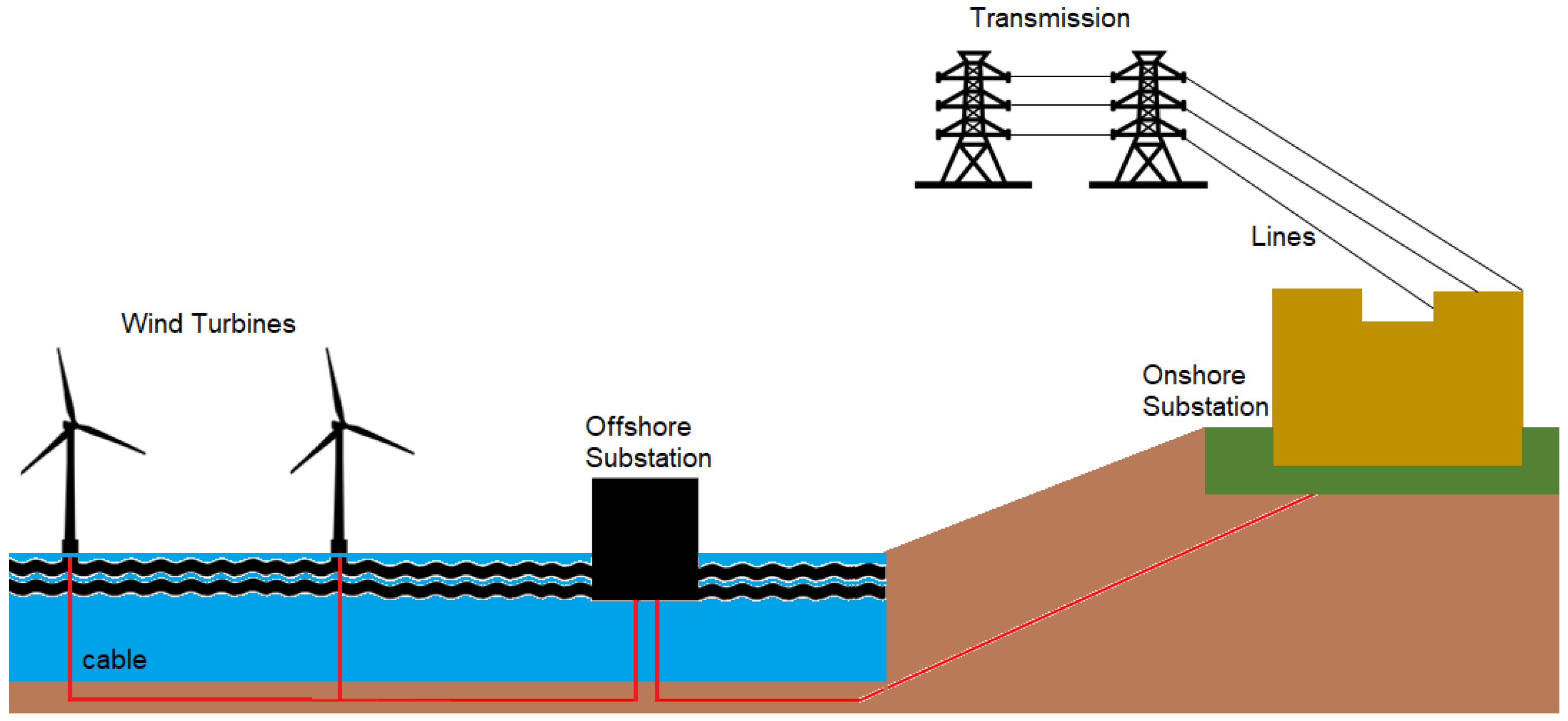Figure 1 shows a simplified scheme of offshore wind energy production.

Generally, wind power generation occurs in three phases, as follows:

• Wind turbines: the blades turn a shaft inside the wind unit. Power energy is produced via a rotational generator (which uses the conversion of magnetic energy into electric);
• Offshore substation: the transformer equipment transforms the power for distribution and delivery to the onshore substation and;
• Lines and grid: power transmission and distribution to consumers.

Active and reactive power dispatch problems are common in the power production area, usually known as optimal power flow (OPF) [6]. Generally, OPF problems have a large dimensional space, and due to their multi-modality, nonlinearity, and non-convexity characteristics, these problems are considered large-scale optimization problems [7]. Solving an OPF consists of finding the more appropriate setups for the controller system (active power and voltages), transformers taps, shunt reactors, and capacitors values [8]. This work addresses an OPF-like problem: A wind power generation problem. We propose an optimal dispatch WPP controller, in which appropriate parameter settings of the algorithm are obtained automatically over time so that its performance is optimized. Several methods and techniques for solving OPF problems have been proposed in the state-of-the-art literature. The advantages and disadvantages associated with the most used methods for solving OPF problems can be found in the works of [6,9,10]. We summarize this information in

Table 1. Methods used to solve electrical dispatch in optimal power flow problems.

Method	Description	Advantages	Disadvantages	Works
Linear	Usage of linear or	Convergence is fast	Inaccuracy due	[11]
Programming	piecewise linear cost	and guaranteed;	to linearization	[12]
	functions and	less computational	of cost funtions
	usage of DC power	effort; easy	and nonlinear
	flow instead	handling of	constraints
	of AC power flow,	inequality constraints
	which provides a
	linear relation between
	injections and
	line flows
Quadratic	Usage of a quadratic	It does not require	Computation cost	[13]
Programming	objective function,	linearization of	can be significantly	[14]
	all constraints	functions	high
	are linear
Meta-heuristics	Genetic Algorithms (GA),	No linearization	The solution	[15]
	Particle Swarm	is required;	obtained is not	[16]
	Optimization (PSO),	uses non-continuos,	guaranteed	[17]
	Differential Evolution (DE),	non convex, and	to be optimal	[18]
	Ant Colony	non differentiable		[19]
	Optimization (ACO)	functions; easy
	are the most	implementation
	applied meta-heuristics

.

Specifically in wind energy production, it is possible to find recent related works in the literature. Kotur and Stefanov [3] proposed an optimal power flow control in a system with offshore wind power plants. Using the IEEE 14-bus system test system, the Interior Point Method was applied to solve the OPF-like problem. The authors concluded that the proposed approach was more efficient than a standard system controller. A mathematical modeling of wind generation was proposed in [4]. The general idea was to minimize costs of wind intermittency using Linear Programming techniques. Results showed that the applied methodology is suitable for quantifying the effects of the shape of the forecast error distribution and the coefficient costs of wind intermittency.

A wind farm control strategy was proposed to maximize the power reserve during de-loading operation while maintaining the total power delivered by the WPP at the point of common coupling (PCC) [20]. The problem was solved by the AEOLUS SimWindFarm (SWF) Simulink toolbox [21]. Sakipour and Abdi [22] proposed a study based on wind power generation testing nine evolutionary algorithms, as Grey Wolf Optimizer (GWO), Artificial Bee Colony (ABC), GA, PSO, and among others. The goal was to find an efficient microgrid configuration using storage systems into a wind farm. Results showed that the GWO performed better, increasing the remaining expected life of batteries in the system.

Self-Adaptive Evolutionary Programming (SAEP) was proposed in [23] to minimize the wind power generation costs. Obtained solutions validated the proposed methodology. Gwabavu and Raji [24] presented a dynamical control system based on model predictive control applying Quadratic Programming to solve the OPF problem. The results showed that the proposed method can reduce grid-connected wind power fluctuations and limit system faults in power generation. Joseph et al. [25] proposed the use of a PSO method to maximize the system loadability within stability margins. Results showed that PSO improved the load carrying capacity when compared to the controller system installed in the plant. Bai et al. [26] applied the ABC algorithm to minimize the production costs on a WPP. A comparison of results between ABC, GA, and PSO was performed, and ABC showed better average results.

Seok and Chen [27] proposed an intelligent wind power plant coalition formation model solved by mathematical programming to achieve profit growth. The authors concluded that the model is especially applicable to heterogeneous WPPs. According to Helmi et al. [28], improving the efficiency of distribution networks is a challenging goal for both large networks and microgrids connected to the public grid. In this context, the Harris Hawks Optimization (HHO) was proposed to minimize power losses of three IEEE systems: 33-bus, 85-bus, and 295-bus. Results showed that HHO performed better than Cuckoo search algorithm (CSA) and PSO for minimizing the losses of systems tested. An optimal network configuration in an active distribution network reduces power loss, improves voltage profile as well as system efficiency and reliability [29]. Thus, the Water Cycle algorithm (WCA) was proposed to reduce the losses of the IEEE 33-bus and IEEE 69-bus systems. WCA outperformed other optimization techniques such as CSA, Harmony Search Algorithm (HSA), and Fireworks Algorithm (FWA). Similar approaches to minimize system loss in wind power plants were proposed in Packiasudha et al. [30] using the Cumulative Gravitational Search Algorithm (CGSA). The minimization of system losses in wind farms was also solved via deterministic algorithms as seen in the works of Huang et al. [31] and Sakar et al. [32].

Pham et al. [33] proposed an optimization method, the Mean-Variance Mapping Optimization (MVMO), to solve the reactive optimal control to WPPs, taking into account the minimization of losses. MVMO was applied to solve the problem using the IEEE 41-bus system as test scenario (available in [34]). Obtained results showed that a fine-tuned MVMO version generated adequate solutions for the OPF-like problem. It is important to say that the IEEE 41-bus system model considers that there is no uncertainty associated with the decision variable values. For dealing with uncertainty in the variables, more complex approaches, such as stochastic or robust optimization methods, are needed. In [35,36], stochastic and a robust approaches were proposed to minimize network losses.

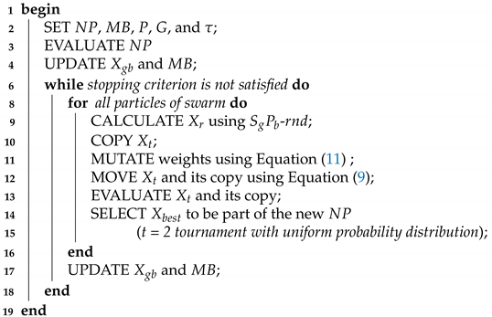
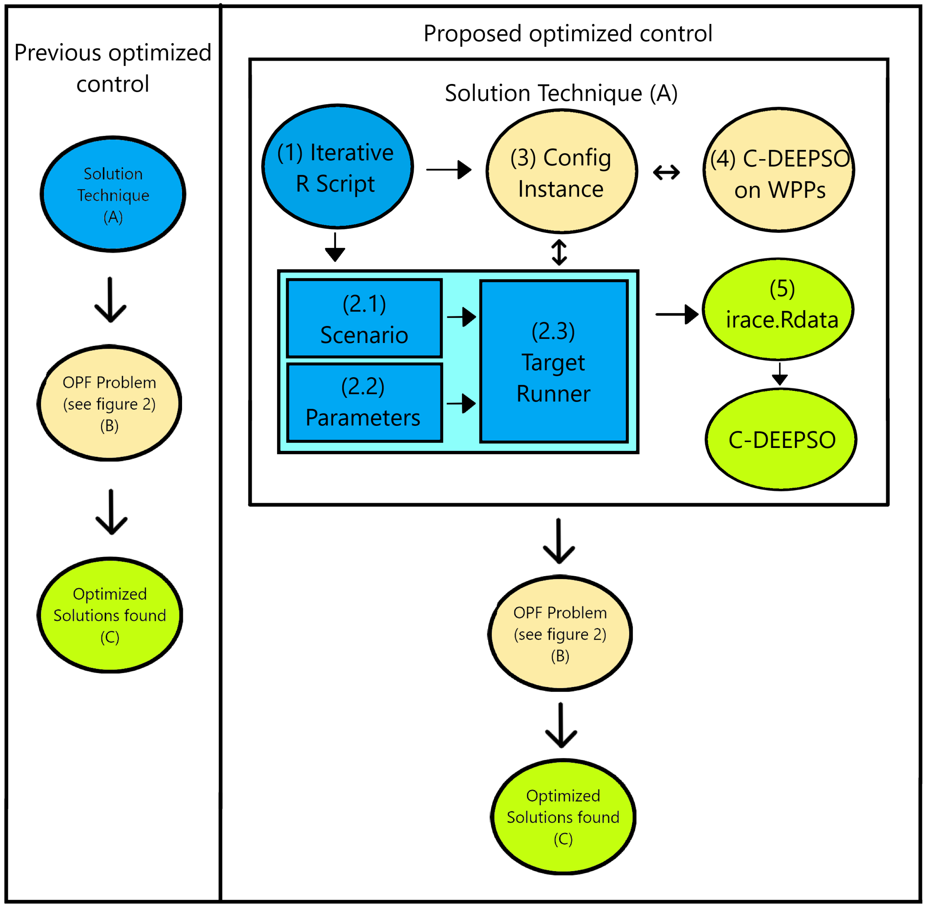
In this work, we solve a dynamic OPF-like problem representing the reactive power dispatch in wind power plants. We propose an integration between the Canonical Differential Evolutionary Particle Swarm Optimization algorithm (C-DEEPSO) [37] and irace [38] as an automatic control system to provide the electric dispatch for WPPs. C-DEEPSO, a hybridization between the particle swarm algorithm and the differential evolution algorithm, was proposed in 2018. The algorithm takes advantage of swarm intelligence methods and the canonical genetic operators of evolutionary computation techniques. Since its proposal, C-DEEPSO has been successfully applied to diverse power systems problems. In general, power system problems such as OPF (optimal power flow) and SCOPF (security constrained optimal power flow) are hard problems to solve, having a high number of distinct optimization variables to optimize and various constraints to deal with. It is well-known that algorithms for solving these types of problems demand a careful design. Motivated by the performance superiority of C-DEEPSO and its variants when applied to such problems (see [37,39,40,41,42,43,44]), C-DEEPSO presents good features and is a viable and competitive method for solving the OPF-like problem in WPP.

However, the C-DEEPSO performance is related to the choice of its main parameters: the weight mutation and the particle communication. Using the irace package as an internal C-DEEPSO mechanism to automatically fine-tune the parameters, we propose a framework capable of establishing an automated controller to carry out the daily electrical dispatch. In the experimental design, 24 h are discretized into 15 min intervals, totalizing 96 test scenarios. The proposed approach finds the best parameter setting yielding the optimal decision variables for each test scenario. Since the daily electrical dispatch problem is solved by breaking it down into 96 sub-problems in a recursive manner, the proposed approach can be seen as a dynamic way of tackling the OPF-like problem in WPP. To the best of our knowledge, this innovation has not yet been found in the state-of-the-art literature. More specifically, this paper presents the following contributions:

• A new electric dispatch controller with automatic adjustment to solve OPF-like problems in WPP;
• A novel framework to fine-tune the parameters of the C-DEEPSO algorithm. For this, the irace package is coupled to the internal mechanism of C-DEEPSO;
• A new approach to compare stochastic algorithms is performed via an application of post hoc tests using the DSCtool in order to validate the statistical robustness of the results;
• An in-depth performance assessment of C-DEEPSO + irace compared to two different algorithms, DEPPSO and MVMO, when solving the OPF-like problem applied to WPPs;
• Obtained results indicate a competitive performance favoring C-DEEPSO in terms of efficiency and accuracy when applied to the OPF-like problem;
• A projection analysis is conducted indicating reduction of the system energy losses around 2.35 MWh per day.

The rest of the paper is structured as follows. Section 2 presents Materials and Methods: the reactive power optimization applied to WPPs; the C-DEEPSO algorithm and the optimal adjustment control are proposed. Section 3 describes the experiments and results. Section 4 carries out a discussion about the obtained results. Finally, Section 5 includes an overall conclusion and future work.

2. Materials and Methods

2.1. Optimal Power Flow Modeling for Reactive Electric Dispatch

In a competitive environment, the active/reactive power dispatch problem can be formulated considering an alternating current representation and solved using the OPF model. Usually, consumers depend on a reliable and secure supply of electricity. Thus, the study of OPF plays an important role in the energy management system in which the entire system operation is supervised at each time interval. Generally, an OPF problem can be formulated minimizing losses in the power production. In addition to this, a variety of formulations that take other features into account has also gained attention in the energy area, such as minimizing costs and pollutant emissions.

Traditionally, OPF is a non-linear, mixed-integer, and difficult-to-solve optimization problem being considered as an NP-hard problem [45]. OPF has equality and inequality constraints that need to be satisfied during the optimization process. Equality and inequality constraints are related to power balance at each node and power flow equations and the operational limits (such as line flows, voltages, and security constraints) [6,9]. This work used as an OPF-like model the well-known IEEE 41-bus system benchmark problem, which characterizes a reactive electrical dispatch problem for an offshore WPP [33].

2.1.1. Optimal Power Flow Formulation

The formulation of OPF for reactive power dispatch aims to minimize the total losses (in MWh) of the energy system.

Table 2. Description of all terms in the mathematical model.

Term	Description
$P_{loss}$	Total losses of the energy system (in MWh)
$NL$	Total number of lines in system
$G_k$	Conductance of line K
U	Voltage magnitude of lines in (in kV): sending end (i); receiving end (j)
$\delta$	Angle of the bus voltages (in degrees)
$P_i$	Active power injected (in MW)
$Q_i$	Reactive power (in MVar)
$\theta$	Voltage angle (in degrees)
$U_i^{min}$, $U_i^{max}$	Bus voltage magnitude in limits minimum and maximum (in kV)
$S_{ij}$	Apparent power flow injection (in MVA)
$T_k$	Tap change limits
$Q_k$	Number of capacitor/reactor banks
$NB$	Number of buses

displays the terms used in the mathematical model.

Equation (1) describes the objective function adopted in the IEEE 41-bus system:

$$\begin{array}{c}\hfill {\displaystyle \mathit{min}{\mathit{P}}_{loss}\left(inMWh\right)=\sum _{K=1}^{{}^{N_L}}{G}_K[U_i^2+U_j^2-2U_i{U}_{j}cos({\delta }_i-{\delta }_j)],}\end{array}$$

(1)

in which the term $N_L$ represents the total number of lines in the system. $G_K$ is the conductance of the line K; $U_i$ and $U_j$ are the magnitudes of the sending end and receiving end voltages of the line. The terms ${\delta }_i$ and ${\delta }_j$ are angles of the bus voltages.

To solve this OPF problem, the optimization algorithm is used as an automatic control to provide an efficient functioning of the WPP according to the input of the reactive power condition of the system. Reactive power is susceptible to failures and losses that must be minimized. Adjustments to minimize losses can be done at the so-called VAR points. The VAR points are inputs to command wind turbines. The input schedules of wind turbines are operated by the WPP control system by allocating the necessary reactive power equally to each generator in the farm.

This optimal reactive power dispatch problem must comply with a group of hard constraints, when the case set conditions for the variables must necessarily be satisfied, or soft set, in which case some variable values can suffer penalization if the conditions are not satisfied. The following set defines the constraints linked to the OPF studied in this work:

• Active (in MW) and Reactive (in MVar) power balance

  $$\begin{array}{c}\hfill P_i=P_i^{gen}-P_i^{load}=\sum _{j=1}^n{U}_i{U}_j[G_{ij}cos({\theta }_i-{\theta }_j)+B_{ij}sin({\theta }_i-{\theta }_j)],\end{array}$$

  (2)

  $$\begin{array}{c}\hfill Q_i=Q_i^{gen}-Q_i^{load}=\sum _{j=1}^n{U}_i{U}_j[G_{ij}sin({\theta }_i-{\theta }_j)-B_{ij}cos({\theta }_i-{\theta }_j)],\end{array}$$

  (3)

  in which $P_i$ is the active power injected, $Q_i$ is the reactive power, $U_i$ is the voltage magnitude, and ${\theta }_i$ is the voltage angle.
• Bus voltage (in kV)

  $$\begin{array}{c}\hfill U_i^{min}\le U_i\le U_i^{max},\end{array}$$

  (4)

  in which $U_i$ corresponds to the bus voltage magnitude vector and its corresponding limits (min and max).
• Branch apparent power flow (in MVA)

  $$\begin{array}{c}\hfill S_{ij}^{min}\le S_{ij}\le S_{ij}^{max},\end{array}$$

  (5)

  in which $S_{ij}$ (MVA) is the apparent power flow injection at the sending end of the transmission circuit connecting bus i to bus j. $S_{ij}^{min}$ and $S_{ij}^{max}$ are the maximum and the minimum limits of apparent power flow.
• Transformer tap

  $$\begin{array}{c}\hfill T_k^{min}\le T_k\le T_k^{max},\end{array}$$

  (6)

  in which $T_k$ corresponds to the vectors of transformer discrete tap change limits (minimum and maximum). The term $T_k$ also means the tap setting position of the On-Load Tap Changer (OLTC).
• Shunt VAR

  $$\begin{array}{c}\hfill Q_k^{min}\le Q_k\le Q_k^{max},\end{array}$$

  (7)

  in which $Q_k$ are capacitor/reactor banks discrete variables.

The penalization of the fitness value of infeasible solutions is a useful approach for treating constraints [42,46,47,48]. Therefore, to meet the constraints, we use the fitness function ($f_p$) provided in the Equation (8):

$$f_p=\left[\begin{array}{cccc}1& 1& 1& 1\end{array}\right]\left[\begin{array}{c}max{(0,P{g}_{REF}-\overline{P{g}_{REF}})}^2+max{(0,\underline{P{g}_{REF}}-P{g}_{REF})}^2\\ {\sum }_{i=1}^{N{B}_{PQ}}{[max(0,U_i-\overline{U_i})+max(0,\underline{U_i})]}^2\\ {\sum }_{i=1}^{NC}{[max(0,\left|S_{ij}\right|-\overline{S_{ij}})+max(0,\left|\begin{array}{c}{S}_{ji}\end{array}\right|-\underline{S_{ij}})]}^2\\ {\sum }_{i=1}^{N{B}_{REF+PU}}{[max(0,Q_i-\overline{Q_i})+max(0,\underline{Q_i}-Q_i)]}^2\end{array}\right].$$

(8)

in which $REF$ is the voltage magnitude, $NB$ is the number of buses, and $NC$ is the number of circuits in the network.

2.1.2. Offshore Wind Power Plant (WPP)

The plant’s components, in general, have to be well organized for the functioning of point of common coupling (PCC). The PCC corresponds to the point in which the generating facility’s local electric power system connects to the utility’s electric system and measures the system losses. Therefore, the task of the proposed WPP optimizer system is to control set points of each generator and the active or passive reactive power compensation equipment, so that control conditions at the PCC are attended. In this work, a version of the WPP modeling (IEEE 41-bus test system) is used to test the robustness of the proposed approach to solve the problem of optimal reactive power dispatch addressed. Figure 2 shows the control scheme of a WPP—a typical topology system. The data about the test network is provided in Appendix A.

From the scheme detailed in Figure 2, the reactors $X_{sh1}$ and $X_{sh2}$ are adjusted continuously; $C_1$ is the capacitor, and it provides support to assist reactive power. The $L1$ term is the active power indicating the load generated by the plant. The reactive power ($q_{ref}$) is provided until it reaches the power of common coupling ($q_{PCC}$) by the controller. Here, the difference between $q_{ref}$ and $q_{PCC}$ for normal is a constraint in which $q_{PCC}$ is the actual reactive power injection at the PCC. The OPF addressed here is considered a mixed-integer problem and is over-contrained. The problem has 22 optimization variables, comprising 18 continuous variables associated with the wind generator reactive power set-points, 02 discrete variables associated with the stepwise adjustable on-load transformers’ tap position, and 02 continuous variables defining the adjustment of shunts ($X_{sh1}$ and $X_{sh2}$).

Table 3. IEEE 41-bus test system characteristics.

IEEE 41-Bus
Test System
Description of test system
	Generators		18
	Linked cable		1
	Transfomers	Fixed tap: T1	33
		Fixed tap: T2	13
Description of the optmization problem		Continuous	18
		variables
	Optimization	Discrete	2
	variables	variables
		Continuous and	2
		stepwise variables
	Constraints system		123

describes the characteristics of the IEEE 41-bus test system and the respective description of the problem taking into account the mathematical formulation described in Section 2.1.1.

2.2. The C-DEEPSO Algorithm

The Canonical Differential Evolutionary Particle Swarm Optimization (C-DEEPSO) [37] is a single-objective algorithm based on the EPSO (Evolutionary Particle Swarm Optimization) [50] and Differential Evolution (DE). C-DEEPSO is an improvement of DEEPSO (see [51,52]). C-DEEPSO has been successfully applied to several optimization problems in power systems, such as: minimization of costs in power production [53], active power dispatch in large scale grids [37], cascade operation in hydropower plants [39], study of energy generation via renewable sources and energy storage systems [41], hybrid microgrid systems operation [43], minimization of active power losses [40], control optimization in hydraulic power plants [44], and pattern classification [54].

C-DEEPSO working mechanisms depend on mutation cycle, recombination, and selection procedures. The idea is to generate a new offspring population such that the overall fitness of the swarm is refined. C-DEEPSO uses a memory archive (Memory B) to use the information archived from previous generations in order to refine the search process. For improving the search assimilation, the movement equation adopted is described by Equations (9) and (10):

$$\begin{array}{c}\hfill V_t=w_I^{*}\times V_{t-1}+w_A^{*}\times (X_{best}+F\times (X_{t-1}-X_r))+w_C^{*}\times \mathcal{C}\times (X_{gb}^{*}-X_{t-1}),\end{array}$$

(9)

$$\begin{array}{c}\hfill X_t=X_{t-1}+V_t,\end{array}$$

(10)

in which $V_t$ is the velocity of the particle, and X is the current solution. $X_{best}$ is the best solution, and $X_{gb}$ the global best solution. The term t means the current generation. $\mathcal{C}$ is a $n\times n$ diagonal matrix that helps the algorithm to escape to a better search region (see [39]). Inertia ($w_I$), assimilation ($w_A$), and communication ($w_C$) are the weights used. $X_r$ is obtained via uniform combination of current and memory populations. Here, we used inspiration from DE algorithm. The DE/best/1 operation is performed inside C-DEEPSO when $X_{t-1}$ is better than $X_r$. In C-DEEPSO, the weights associated with inertia, assimilation, and communication are changed accordingly to Equation (11):

$$\begin{array}{c}\hfill w^{*}=w+\tau \times \mathcal{N}(0,1),\end{array}$$

(11)

in which $\tau$ represents the mutation rate. C-DEEPSO uses a Gaussian Distribution ($N(0,1)$) to move slightly the current solution in the search space.

The global best solution $X_{gb}$ is mutated in order to attract the current individual as next as possible to a attracting promising bay of solutions. The current individual is then slightly moved in the search space using a Gaussian Distribution. The term $X_{gb}$ is mutated using the Equation (12):

$$\begin{array}{c}\hfill X_{gb}^{*}=X_{gb}[1+\tau \times \mathcal{N}(0,1)].\end{array}$$

(12)

C-DEEPSO pseudo-code is shown in Algorithm 1, in which $NP$ is the population size, $MB$ is the memory archive size, and G means generations used. The terms P and $\tau$ are the communication probability and is the mutation rates, respectively.

Algorithm 1:C-DEEPSO algorithm.

2.3. Optimal Adjustment Control Proposed: C-DEEPSO Integrated with irace Package

The electrical dispatch referring to one day (24 h) has been discretized into 15 min intervals, resulting in 96 test scenarios to be solved. Our proposal is to perform the dynamic dispatch of the system performing the automatic adjustment of the C-DEEPSO algorithm. To achieve this goal, we have integrated the irace package within the C-DEEPSO algorithm to automatically adjust the rates of its main operators: mutation and communication. This measure is in line with good practices for carrying out fine-tuning of parameters to evolutionary algorithms.

The fine-tuning process is a methodology that is applied to find the best configurations of parameters considering a set of possible values for the parameters for each problem. We have performed the fine-tuning process using irace tool [38]. The irace is an R package that is able to automatically configure an algorithm when its performance depends on the choice of the parameter settings.

As the OPF problem is both dynamic and a blackbox problem (IEEE 41-bus system), we have created an interface between irace and the Matlab script implementing the C-DEEPSO algorithm. This interface calls C-DEEPSO, runs it only one time in the problem requested by the irace, and returns the best fitness value. The irace package then makes a series of statistical comparisons using hypothesis tests (to check, for instance, mean differences). In our experimental design, we are looking for the best rates for Communication and Mutation Probability parameters for each test scenario.

The irace iterates, for each one of the 96 scenarios, all the possible configurations of mutation probability and communication rate and compares them, excluding the ones that are proven statistically worse. In the end of the iterations, the irace returns a dataframe with all tested configurations (ordered as tested) and a list of the best configurations, called elite configurations. This dataframe, called irace.Rdata, also has a list of rejected configurations that are proven statistically worse than the elite configurations. Figure 3 exemplifies the proposed optimal controller in action. The previous (or classical) optimized control is composed by an optimization algorithm (A), such as DEEPSO, MVMO, or other, that solves the OPF problem (B) and finds an optimized solution (C). In our proposed optimized control, we conduct a process that finds the best parameter configuration for C-DEEPSO algorithm before running it on the OPF-like problem, to obtain the optimized solutions via C-DEEPSO for solving the electric dispatch in a WPP.

3. Experiments and Results

The experimental part of this work is carried out under the observation of the daily electrical dispatch. Generally, when planning the electrical dispatch operation, the seasonality of the region in relation to the generating source must be taken into account. According to Arce et al. [55], the main stages of dispatch operation planning, taking into account seasonality, are: long (several-year horizon), medium (one-year horizon), short-term (one-week horizon), daily (one day), and in real time. In this work, we have chosen to carry out a study under the bias of daily planning of electrical dispatch operation in a wind power plant (WPP). This approach is justified by the fact of having in hand data for only one day testing in IEEE 41 Bus-System. The main rationale behind our choice has been the possibility of a performance comparison among the proposed approach and the two state-of-the-art approaches, DEEPSO and MVMO.

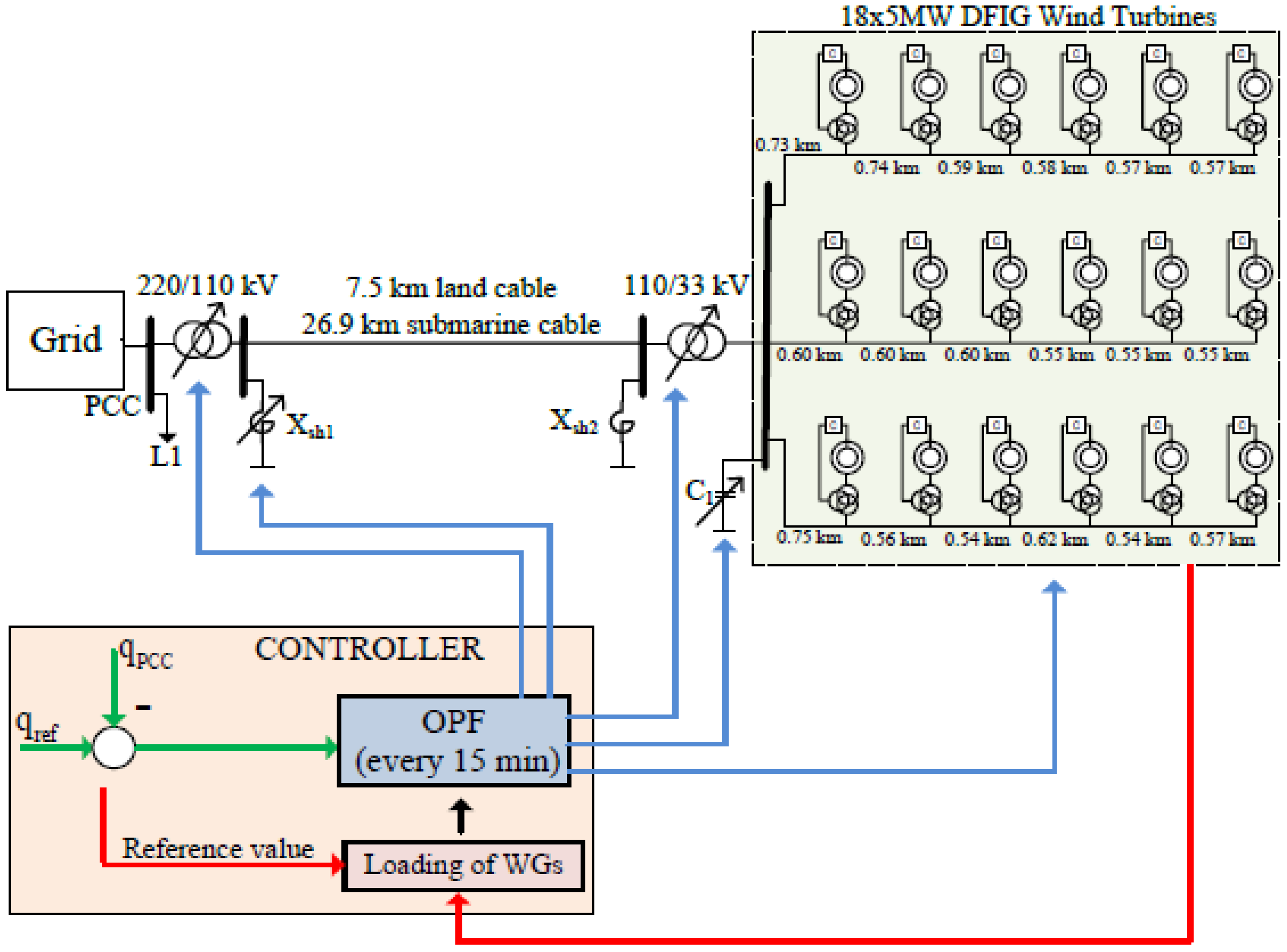
The electrical dispatch in WPPs discussed in this work is dynamic in nature. To handle its dynamicity, we use an integration between C-DEEPSO and irace, which works like an optimized automatic controller. The WPP system has 18 generators (5 MW) that are connected to the transformers (100 MVA) and the grid (220 kV) through a submarine cable (110 kV—around 30 km length). The transformers provide OLTC service and operate T1 (% kV with 33 taps and 220 kV to PCC) and T2 with 13 taps. There is no equality in the distances between the generators and the WPP main collector. Wind turbine terminals need to be maintained between 0.92 and 0.97 kV (which corresponds 920–970 V). The nominal voltage value is 0.95 kV (950 V). The system also has a shunt reactor adjusted with ON/OFF control (500 $\Omega$) to adequate the excessive charging of the submarine cable.

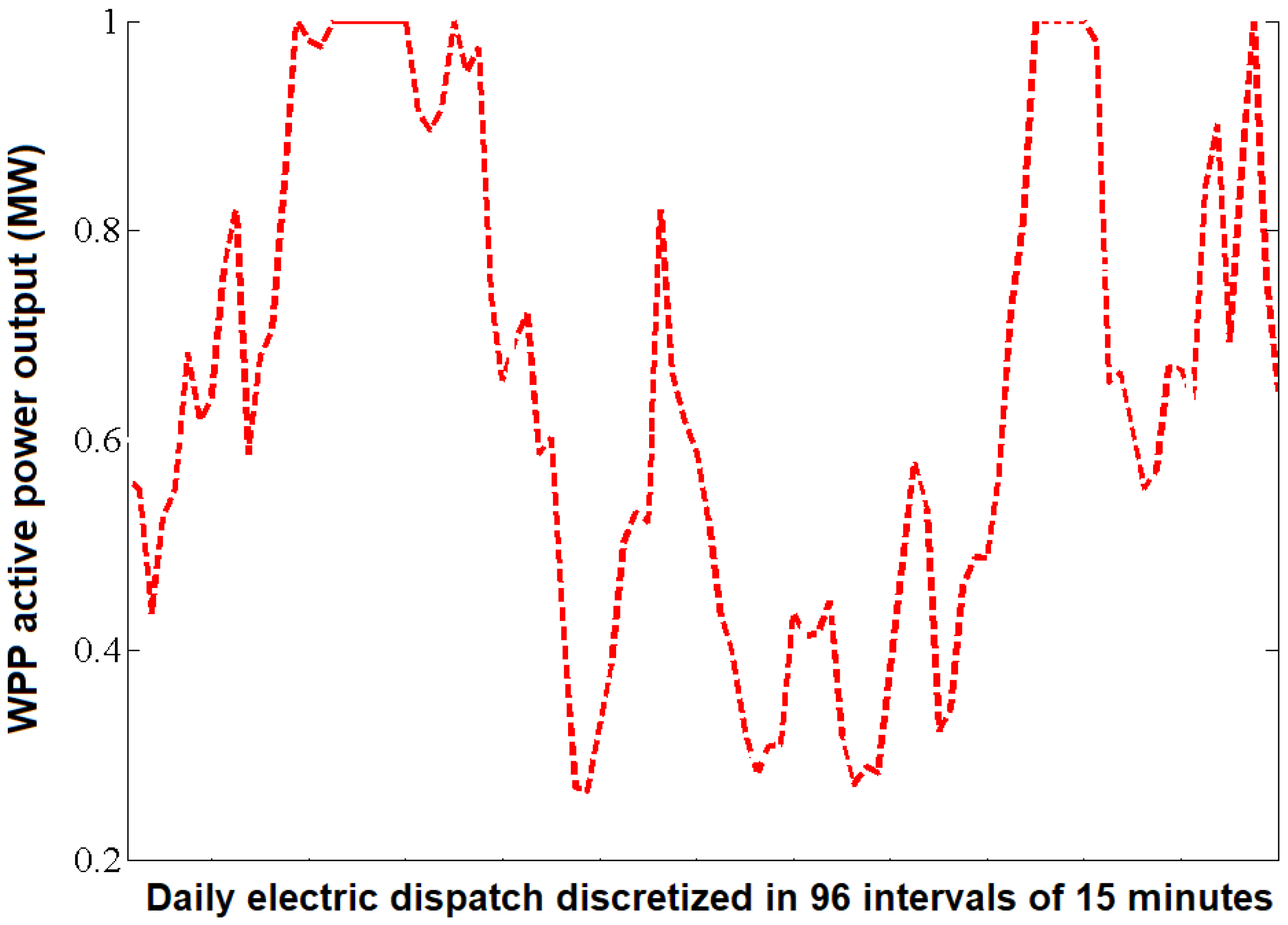
The goal is to provide optimized sets of all VAR sources to meet the actual reactive power requirement at PCC including: the individual reactive power of each wind turbine, OLTC adjustments, and shunt reactor ON/OFF positions. The controller calculates the optimal adjustment in intervals of 15 min, in a total of 96 intervals, for which the reactive electric dispatch must be solved. Simulation has been done to show the reactive power control problem, which is defined by progressive changes in the necessary reactive power ($q_{ref}$). The experimental design contemplates over a period of one day (24 h discretized to in intervals of 15 min). Figure 4 shows a typical WPP output.

A control strategy must be carried out to ensure system availability and to continuously meet reactive power ($q_{ref}$). Here, the adopted experimental design is used to show that C-DEEPSO is able to solve the OPF-like problem addressed, respecting the constraints. C-DEEPSO was runned 31 times in each one of the 96 intervals of power production. The computational simulation was done using an Intel i9 3.7 Ghz and 64 GB de RAM on Ubuntu 20.04.2.0 LTS Operating System computer. The code was implemented in Matlab using the MATPOWER package. The integration of R (4.1.1) and Matlab was done with a Python (3.7) script.

To validate our proposal, the performance of C-DEEPSO integrated with irace is compared to the performance of DEEPSO and MVMO algorithms. Since C-DEEPSO has been derived from DEEPSO, the comparison between those algorithms also aims to see if the improvements brought by C-DEEPSO are relevant. On the other hand, MVMO is the reference algorithm for this problem. DEEPSO and MVMO [33] results have been extracted from [34], where they were used in their best parameter configuration. 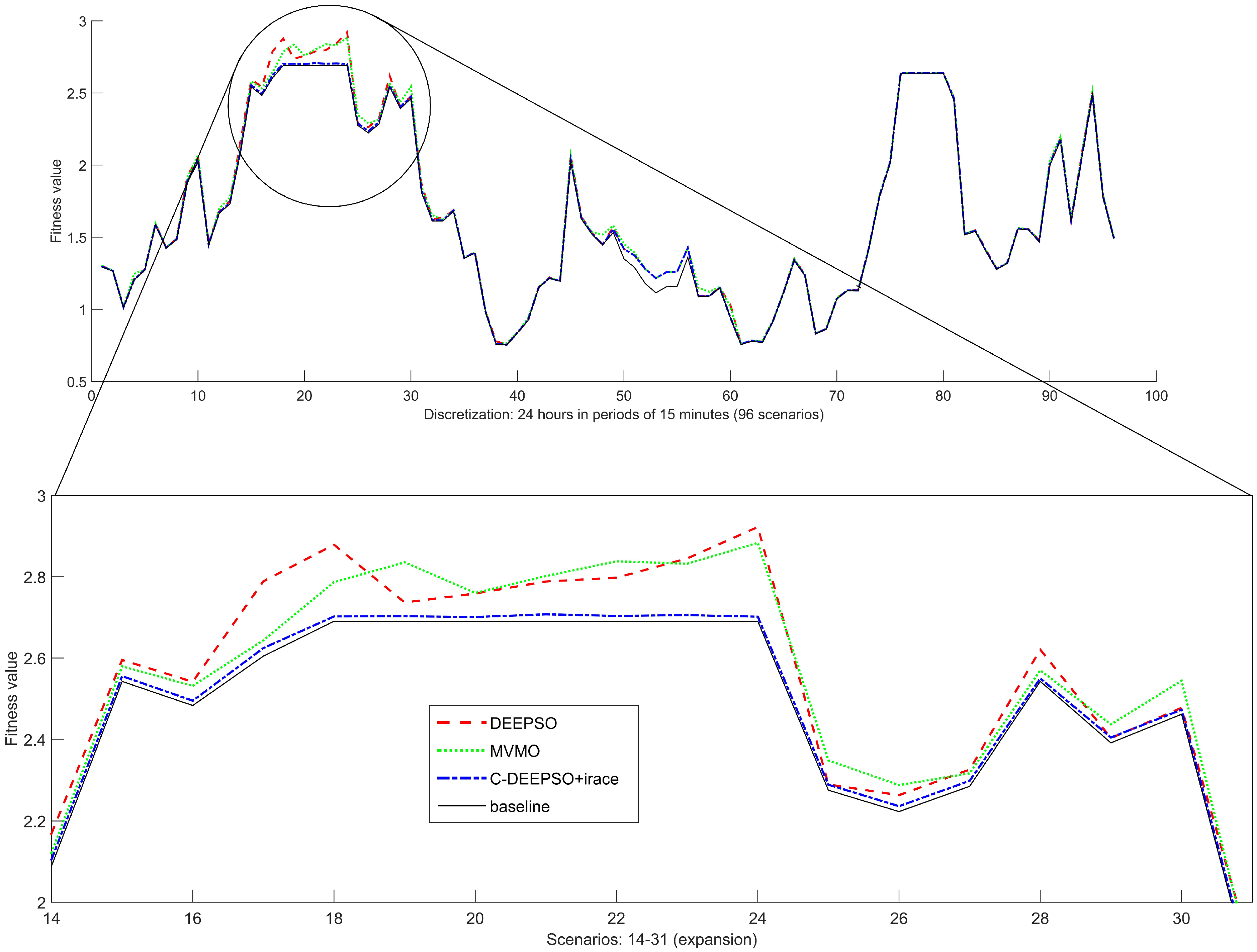Figure 5 shows the result obtained by each tested algorithm: C-DEEPSO + irace, DEEPSO, and MVMO. The graph presents the range of all scenarios, emphasizing cases 14–31 in its expansion. C-DEEPSO shows the best result among the tested methods.

The irace package implements the iterated racing methodology [38], a method for automatic configuration with steps: (1) sampling new configurations according to a particular distribution; (2) selecting the best configurations from the newly sampled ones by means of racing; and (3) updating the sampling distribution in order to bias the sampling towards the best configurations.

Table 4. Comparative result of the C-DEEPSO + irace, DEEPSO and MVMO algorithms. Legend: scenario (Sc.) is the number of each measured interval of energy production (96); significance (S.) with $\alpha =5\%$ on Kolmogorov–Smirnov test (“+” reject null hypothesis of mean difference and “=” not reject the null hypothesis); optimal mutation rate found (Mut.); optimal communication rate found (Com.); mean (mean results of 31 runs); STD (standard deviation of 31 runs).

		C-DEEPSO + irace				DEEPSO		MVMO
Sc.	S. (5%)	Mut.	Com.	AVR	STD	AVR	STD	AVR	STD
1	(+)	0.70	0.50	1.2961	0.0063	1.3004	0.0065	1.2995	0.0021
2	(+)	0.30	0.40	1.2670	0.0007	1.2737	0.0068	1.2709	0.0025
3	(+)	0.50	0.20	1.0137	0.0032	1.0185	0.0091	1.0180	0.0062
4	(+)	0.90	0.50	1.2061	0.0016	1.2104	0.0067	1.2142	0.0125
5	(+)	0.10	0.30	1.2745	0.0012	1.2774	0.0049	1.2775	0.0030
6	(+)	0.40	0.40	1.5893	0.0013	1.5907	0.0024	1.5950	0.0030
7	(+)	0.60	0.90	1.4272	0.0021	1.4306	0.0039	1.4317	0.0034
8	(+)	0.50	0.40	1.4864	0.0023	1.4901	0.0027	1.4912	0.0018
9	(+)	0.70	0.50	1.8886	0.0067	1.9206	0.0251	1.9127	0.0177
10	(+)	0.60	0.70	2.0370	0.0068	2.0599	0.0210	2.0681	0.0248
11	(+)	0.90	0.80	1.4493	0.0018	1.4605	0.0192	1.4668	0.0288
12	(+)	0.20	0.10	1.6732	0.0021	1.6879	0.0092	1.6967	0.0202
13	(+)	0.10	0.10	1.7389	0.0060	1.7545	0.0092	1.7653	0.0197
14	(+)	0.60	0.80	2.1052	0.0067	2.1385	0.0232	2.1313	0.0158
15	(+)	0.60	0.50	2.5555	0.0096	2.5764	0.0157	2.5835	0.0178
16	(+)	0.70	0.30	2.4950	0.0081	2.5230	0.0226	2.5268	0.0157
17	(+)	0.70	0.40	2.6245	0.0127	2.7631	0.0632	2.7530	0.0497
18	(+)	0.70	0.30	2.7023	0.0155	2.8377	0.0498	2.8328	0.0653
19	(+)	0.60	0.40	2.7028	0.0139	2.8389	0.0547	2.8321	0.0596
20	(+)	0.90	0.30	2.7010	0.0185	2.8295	0.0629	2.8368	0.0379
21	(+)	0.50	0.10	2.7075	0.0225	2.8264	0.0541	2.8243	0.0522
22	(+)	0.70	0.30	2.7038	0.0204	2.8400	0.0420	2.8105	0.0433
23	(+)	0.80	0.40	2.7057	0.0174	2.8492	0.0521	2.8130	0.0604
24	(+)	0.90	0.30	2.7018	0.0162	2.8246	0.0604	2.8306	0.0384
25	(+)	0.50	0.70	2.2891	0.0017	2.3205	0.0267	2.3284	0.0260
26	(+)	0.90	0.80	2.2363	0.0085	2.2791	0.0185	2.2739	0.0227
27	(+)	0.90	0.50	2.2987	0.0008	2.3322	0.0199	2.3268	0.0164
28	(+)	0.70	0.50	2.5500	0.0051	2.5840	0.0246	2.5884	0.0252
29	(+)	0.90	0.70	2.4046	0.0047	2.4348	0.0256	2.4355	0.0167
30	(+)	0.60	0.70	2.4728	0.0041	2.5042	0.0195	2.5105	0.0216
31	(+)	0.90	0.90	1.8216	0.0095	1.8371	0.0133	1.8455	0.0319
32	(+)	0.50	0.30	1.6190	0.0032	1.6326	0.0126	1.6384	0.0242
33	(+)	0.40	0.70	1.6158	0.0020	1.6206	0.0055	1.6215	0.0022
34	(=)	0.10	0.80	1.6868	0.0026	1.6888	0.0039	1.6901	0.0024
35	(=)	0.30	0.90	1.3567	0.0022	1.3586	0.0032	1.3593	0.0035
36	(+)	0.70	0.80	1.3935	0.0016	1.3961	0.0032	1.3979	0.0039
37	(+)	0.90	0.90	0.9846	0.0011	0.9891	0.0080	0.9863	0.0023
38	(+)	0.50	0.90	0.7589	0.0015	0.7652	0.0154	0.7616	0.0024
39	(=)	0.40	0.80	0.7549	0.0015	0.7603	0.0126	0.7578	0.0031
40	(=)	0.30	0.90	0.8379	0.0008	0.8402	0.0071	0.8419	0.0053
41	(+)	0.40	0.40	0.9269	0.0136	0.9272	0.0073	0.9272	0.0039
42	(+)	0.80	0.50	1.1522	0.0003	1.1555	0.0052	1.1555	0.0023
43	(+)	0.90	0.70	1.2172	0.0012	1.2209	0.0065	1.2215	0.0044
44	(+)	0.80	0.40	1.1964	0.0012	1.2018	0.0099	1.1997	0.0022
45	(+)	0.70	0.80	2.0350	0.0061	2.0626	0.0186	2.0708	0.0257
46	(+)	0.60	0.10	1.6322	0.0026	1.6450	0.0100	1.6557	0.0256
47	(+)	0.90	0.60	1.5231	0.0019	1.5351	0.0109	1.5530	0.0339
48	(+)	0.80	0.30	1.4491	0.0012	1.4647	0.0211	1.4668	0.0220
49	(+)	0.50	0.80	1.5546	0.0004	1.5732	0.0143	1.5935	0.0382
50	(+)	0.90	0.50	1.4189	0.0001	1.4217	0.0040	1.4298	0.0155
51	(+)	0.80	0.90	1.3725	0.0001	1.3730	0.0006	1.3795	0.0097
52	(=)	0.80	0.90	1.2804	0.0000	1.2803	0.0000	1.2804	0.0001
53	(+)	0.70	0.80	1.2160	0.0000	1.2160	0.0001	1.2161	0.0001
54	(=)	0.70	0.90	1.2579	0.0000	1.2578	0.0000	1.2578	0.0000
55	(=)	0.60	0.90	1.2610	0.0000	1.2611	0.0000	1.2611	0.0000
56	(+)	0.60	0.70	1.4257	0.0001	1.4279	0.0029	1.4352	0.0164
57	(+)	0.80	0.50	1.0896	0.0013	1.1006	0.0192	1.1134	0.0098
58	(+)	0.80	0.70	1.0940	0.0057	1.1071	0.0241	1.1287	0.0379
59	(+)	0.40	0.30	1.1506	0.0027	1.1626	0.0252	1.1852	0.0330
60	(+)	0.90	0.50	0.9422	0.0012	0.9676	0.0411	0.9699	0.0126
61	(+)	0.90	0.40	0.7590	0.0009	0.7683	0.0195	0.7642	0.0098
62	(+)	0.90	0.60	0.7825	0.0079	0.7859	0.0103	0.7883	0.0133
63	(+)	0.90	0.50	0.7726	0.0010	0.7820	0.0185	0.7800	0.0126
64	(+)	0.90	0.50	0.9194	0.0007	0.9249	0.0168	0.9238	0.0095
65	(+)	0.90	0.90	1.1182	0.0007	1.1215	0.0043	1.1202	0.0024
66	(+)	0.90	0.50	1.3421	0.0012	1.3444	0.0022	1.3445	0.0014
67	(+)	0.40	0.90	1.2360	0.0013	1.2396	0.0048	1.2393	0.0013
68	(+)	0.40	0.70	0.8317	0.0009	0.8387	0.0145	0.8341	0.0036
69	(+)	0.50	0.70	0.8642	0.0044	0.8690	0.0106	0.8660	0.0021
70	(+)	0.50	0.80	1.0739	0.0006	1.0766	0.0045	1.0757	0.0015
71	(+)	0.50	0.70	1.1317	0.0005	1.1339	0.0031	1.1344	0.0041
72	(+)	0.70	0.70	1.1299	0.0004	1.1329	0.0034	1.1324	0.0028
73	(=)	0.50	0.10	1.4195	0.0016	1.4244	0.0035	1.4223	0.0021
74	(+)	0.90	0.60	1.7804	0.0041	1.7891	0.0250	1.7833	0.0038
75	(+)	0.80	0.80	2.0113	0.0003	1.2987	0.0018	2.0223	0.0030
76	(+)	0.90	0.50	2.6373	0.0000	1.2964	0.0010	2.6373	0.0000
77	(=)	0.20	0.20	2.6373	0.0000	1.2972	0.0018	2.6373	0.0000
78	(+)	0.30	0.40	2.7373	0.0000	1.2963	0.0010	2.6373	0.0000
79	(=)	0.80	0.30	2.6373	0.0000	1.2974	0.0020	2.6373	0.0000
80	(=)	0.30	0.40	2.6373	0.0000	2.6373	0.0000	2.6373	0.0000
81	(+)	0.70	0.20	2.4610	0.0012	2.4738	0.0373	2.4637	0.0070
82	(+)	0.80	0.80	1.5201	0.0017	1.5227	0.0030	1.5248	0.0022
83	(+)	0.40	0.50	1.5445	0.0017	1.5465	0.0030	1.5493	0.0020
84	(+)	0.60	0.90	1.4070	0.0022	1.4095	0.0026	1.4096	0.0013
85	(+)	0.10	0.90	1.2795	0.0019	1.2822	0.0035	1.2819	0.0012
86	(+)	0.60	0.90	1.3203	0.0028	1.3238	0.0033	1.3229	0.0018
87	(+)	0.10	0.50	1.5585	0.0014	1.5608	0.0025	1.5635	0.0014
88	(+)	0.10	0.90	1.5526	0.0018	1.5546	0.0022	1.5574	0.0020
89	(+)	0.40	0.50	1.4724	0.0012	1.4757	0.0034	1.4769	0.0017
90	(+)	0.20	0.70	2.0066	0.0026	2.0119	0.0068	2.0221	0.0063
91	(+)	0.80	0.70	2.1807	0.0004	2.1924	0.0126	2.1981	0.0053
92	(=)	0.30	0.60	1.6123	0.0018	1.6172	0.0024	1.6223	0.0032
93	(+)	0.80	0.90	2.0554	0.0059	2.0642	0.0102	2.0719	0.0052
94	(+)	0.60	0.90	2.4899	0.0043	2.5161	0.0236	2.5123	0.0071
95	(+)	0.60	0.80	1.7829	0.0015	1.7849	0.0036	1.7923	0.0050
96	(+)	0.80	0.40	1.4976	0.0016	1.5001	0.0022	1.5030	0.0028
		Total		38.01 (MWh)		38.80 (MWh)		40.35 (MWh)

shows the algorithms’ results in terms of average (AVR) and standard deviation (STD). The configurations of Mutation and Communication rates found by irace are also displayed. As can be seen in Table 4, C-DEEPSO coupled to irace obtained, after the iterated racing process, a specific set of parameters for each test scenario.

Results from 31 runs of each algorithm show that C-DEEPSO has the lowest average in 100% of cases tested. To show the efficiency of C-DEEPSO, we carried out a more complete statistical analysis. We used a new tool to perform a post hoc Kolmogorov–Smirnov test to perform a hypothesis test about mean differences, the DSCTool [56]. We compared the results of the algorithms in order to rank them for each of the problem instances using DSCTool. DSCTool is a statistical tool used to compare the performance of algorithms under different scenarios. We applied the DSCTool with the Kolmogorov–Smirnov test with 95% confidence to compare the results of C-DEEPSO against the MVMO and DEEPSO algorithms for all 96 instances of the WPP problem. The algorithms have been ranked as shown in Table 4. (Aiming to allow reproducibility and extension of our results, an online publicly repository is made available at https://github.com/jvcavancini/C-DEEPSO (accessed on 17 October 2021). It contains our proposed approach (C-DEEPSO + irace), the WPP model, and a.csv file containing the optimal decision variable values for each test scenario, corresponding to the median solution over the 31 runs.)

4. Discussion

We adopted an $\alpha =5\%$ (significance level) to conduct the inference statistical test. In each power production interval (in a total of 96), if the Kolmogorov–Smirnov test finds a significant difference between the mean of algorithms, the DSCtool provides the ranking among of algorithm performances. Table 4 shows the signal of statistical test realized: (+) exists differences among the means of algorithms with confidence of 95%, and (=) null hypothesis of equality of means is rejected. In our analysis, 84 test cases (87% of them, respectively) show that there are differences among the algorithm means. However, in 12 out of 96 scenarios, or in 12.5% of the scenarios, the Kolmogorov–Smirnov test was unable to reject the null hypothesis.

Thus, we can say that C-DEEPSO + irace has results with greater robustness when compared to the others in 87% of cases. Observe that C-DEEPSO + irace shows a lower mean value and presents the maximum ranking in the Kolmogorov–Smirnov test, as shown in Table 4 with symbol (+). In the remaining 12 scenarios, the null hypothesis cannot be rejected, showing that there is no statistical significance in the difference of the algorithm means when compared to DEEPSO (indicated by the symbol (=) symbol in Table 4). To summarize, in 87.5% of the test cases, C-DEEPSO + irace is the most efficient algorithm when compared to DEEPSO. In 12.5% of the test cases, C-DEEPSO + irace and DEEPSO are tied in the first position. It is worthwhile to notice that, in all 96 scenarios, C-DEEPSO + irace shows a low average in comparison to MVMO (state-of-the-art algorithm). Therefore, we can say that MVMO is always classified in the third position for solving the OPF-like problem addressed in this work.

Therefore, we consider that C-DEEPSO + irace is an effective method to solve the electric dispatch problem performing an optimal control of the WPP. C-DEEPSO minimizes the transmission losses. Furthermore, it complies with PCC power requirements ensuring the adjustment of all correlated variables. Observe that DEEPSO and MVMO use a single set of optimal parameters considering the whole time scenario. The novelty of the proposed approach is to treat the OPF-like problem in WPP as having a dynamic optimal set of parameters. Integrating irace with C-DEEPSO, the optimal parameters have been adjusted for each of the 96 test cases. This dynamic parameter configuration is responsible for the optimized performance of the proposed approach. C-DEEPSO has proved to be efficient and competitive for solving the problem in a dynamic way. Our algorithm works as a joint electrical dispatch control that learns from the system’s input data at each measured time interval. irace identifies the best mutation and communication rates at each time interval, ensuring the robustness of the proposed system controller.

The total sum of losses is shown in Table 4 for each algorithm. The proposed approach presents a cumulative daily average value of 38.01 MWh per day, while DEEPSO and MVMO present 38.80 MWh and 40.35 MWh, respectively. As shown, the decrease in daily cumulative value is approximately 3% compared to C-DEEPSO and 6% in relation to MVMO. The statistical tests indicate these values show significant improvements. Considering C-DEEPSO + irace and the reference algorithm, MVMO, there is a difference of 2.35 MWh per day, favoring the C-DEEPSO + irace. In a monthly projection, we would have a total loss of $70.02$ MWh per day, supporting the C-DEEPSO + irace.

5. Conclusions

Recent works have shown that wind and solar power have become viable energy sources in developing countries to serve as a sustainable way to produce electricity. The electric dispatch problem in wind power plants can be expressed as an OPF-like problem, in which the goal is to minimize the cost losses of a WPPs. In this work, we used an integrated methodology to minimize reactive power losses in the transmission network in wind farms (OPF-like), coupling C-DEEPSO and irace package (in a fine-tuning methodology). The C-DEEPSO + irace incorporates a single-objective meta-heuristic, implementing some procedures of Swarm Intelligence and Evolutionary Computation. In the proposed approach, the daily dispatch (24 h) was discretized into 15 min intervals, totalizing 96 test scenarios. For each test scenario, irace finds the best parameter configuration for the mutation and communication rates and C-DEEPSO finds the optimal decision variables yielding the minimization of the power losses. The problem is solved in a recursive way and can be seen as an automatic controller for the problem. Using the IEEE 41-bus test system, the proposed algorithm was compared to two other algorithms: DEEPSO and MVMO. Both algorithms were at their best performance with the set of best parameters optimized by their proponents. The results indicated that the proposed C-DEEPSO + irace algorithm outperformed its competitors, being statistically superior when dealing with hard OPF-like problems in WPP.

Although being a very promising approach, the proposed methodology has some limitations that can be addressed in future works. The problem can be solved using long- or medium-term electrical dispatch planning. Different objective criteria such as the minimization of the overall costs can be applied for solving the problem. The irace can also be coupled with a multi-objective evolutionary algorithm for solving the OPF-like problem, taking into account the two or more objective functions simultaneously. Finally, the IEEE 41-bus system model considers that there is no uncertainty associated with the decision variable values; however, a robustness analysis is an important aspect to be analyzed.

References

1. Nations, U. Paris Agreement. Available online: https://unfccc.int/process-and-meetings/the-paris-agreement/the-paris-agreement (accessed on 5 July 2021).
2. Huang, K.; Xu, L.; Liu, G. A Diode-MMC AC/DC Hub for Connecting Offshore Wind Farm and Offshore Production Platform. Energies 2021, 14, 3759. [Google Scholar] [CrossRef]
3. Kotur, D.; Stefanov, P. Optimal power flow control in the system with offshore wind power plants. Int. J. Electr. Power Energy Syst. 2019, 105, 142–150. [Google Scholar] [CrossRef]
4. Jabr, R.; Pal, B. Intermittent wind generation in optimal power flow dispatching. IET Gener. Transm. Distrib. 2009, 3, 66–74. [Google Scholar] [CrossRef]
5. Bhattacharya, S.; Biswal, S.; Aleem, M.; Amani, S.; Prabhakaran, A.; Prakhya, G.; Lombardi, D.; Mistry, H. Seismic Design of Offshore Wind Turbines: Good, Bad and Unknowns. Energies 2021, 14, 3496. [Google Scholar] [CrossRef]
6. Frank, S.; Steponavice, I.; Rebennack, S. Optimal power flow: A bibliographic survey (I)—For deterministics methods and deterministic methods. Energy Syst. 2012, 3, 221–258. [Google Scholar] [CrossRef]
7. Abido, M. Optimal power flow using particle swarm optimization. Electr. Power Energy Syst. 2002, 24, 563–571. [Google Scholar] [CrossRef]
8. Bhaskar, M.; Muthyala, S.; Maheswarapu, S. Security Constraint Optimal Power Flow (SCOPF)—A compreensive Survey. Int. J. Comput. Appl. 2010, 2, 42–52. [Google Scholar] [CrossRef]
9. Frank, S.; Steponavice, I.; Rebennack, S. Optimal power flow: A bibliographic survey (II)—Non-deterministics and hybrid methods. Energy Syst. 2012, 3, 259–289. [Google Scholar] [CrossRef]
10. Pandya, K.; Joshi, S. A Survey of optimal power flow methods. J. Theor. Appl. Inf. Technol. 2008, 4, 450–458. [Google Scholar]
11. Rau, N. Issues in the path toward an RTO and standard markets. IEEE Trans. Power Syst. 2003, 18, 435–443. [Google Scholar] [CrossRef]
12. Stott, B.; Jardim, J.; Alsac, O. DC power flow revisited. IEEE Trans. Power Syst. 2009, 24, 1290–1300. [Google Scholar] [CrossRef]
13. Horst, R.; Pardalos, P.; Thoai, N. Introduction to Global Optimization, 2nd ed.; Springer: New York, NY, USA, 2000. [Google Scholar]
14. Burchett, R.; Happ, H.; Wirgau, K. Large scale optimal power flow. IEEE Trans. Appar. Syst. 1982, 101, 3722–3732. [Google Scholar] [CrossRef]
15. Teng, J.; Liu, Y. A novel ACS-based optimum switch relocation method. IEEE Trans. Power Syst. 2003, 18, 113–120. [Google Scholar] [CrossRef]
16. Gasbaoui, B.; Allaoua, B. Ant colony optimization applied on combinatorial problem for optimal power flow solution. Leonardo J. Sci. 2009, 14, 1–17. [Google Scholar]
17. Aminudin, N.; Rahman, T.; Musirin, I. Optimal power flow for load margin improvement using evolutionary programming. In Proceedings of the 5th Student Conference on Research and Development (SCOReD2007), Selangor, Malaysia, 11–12 December 2007; Volume 1, pp. 1–6. [Google Scholar] [CrossRef]
18. Liang, C.; Chung, C.; Wong, K.; Duan, X.; Tse, C. Study of differential evolution for optimal reactive power flow. IET Gener. Transm. Distrib. 2007, 1, 253–260. [Google Scholar] [CrossRef]
19. Yumbla, P.; Ramirez, J.; Coello, C. Optimal power flow subject to security constraints solved with a particle swarm optimizer. IEEE Trans. Power Syst. 2008, 23, 33–40. [Google Scholar] [CrossRef]
20. Siniscalchi-Minna, S.; Bianchi, F.; De-Prada-Gil, M.; Ocampo-Martinez, C. A wind farm control strategy for power reserve maximization. Renew. Energy 2019, 131, 37–44. [Google Scholar] [CrossRef]
21. Grunneta, J.; Soltani, M.; Knudsen, T.; Kragelund, M.; Bak, T. Aeolus toolbox for dynamics wind farm model, simulation and control. In Proceedings of the European Wind Energy Conference & Exhibition, Warsaw, Poland, 20–23 April 2010; Volume 1, pp. 1–8. [Google Scholar]
22. Sakipour, R.; Abdi, H. Optimizing Battery Energy Storage System Data in the Presence of Wind Power Plants: A Comparative Study on Evolutionary Algorithms. Sustainability 2020, 12, 10257. [Google Scholar] [CrossRef]
23. Shi, L.; Xu, G. Self-adaptive evolutionary programming and its application to multi-objective optimal operation of power systems. Electr. Power Syst. Res. 2001, 57, 181–187. [Google Scholar] [CrossRef]
24. Gwabavu, M.; Raji, A. Dynamic Control of Integrated Wind Farm Battery Energy Storage Systems for Grid Connection. Sustainability 2021, 13, 3112. [Google Scholar] [CrossRef]
25. Joseph, S.; Skariah, E.; Joseph, T.; Sreedharan, S.; Chittesh, C.; Vipin, P.; Vishnu, J. PSO Based Controller Algorithm for Optimal Allocation & Setting of Fuel Cell in a Wind—PV Integrated Power System for Maximizing Loadability. In Proceedings of the 2014 International Conference on Advances in Green Energy (ICAGE), Thiruvananthapuram, India, 17–18 December 2014; Volume 1, pp. 1–8. [Google Scholar] [CrossRef]
26. Bai, W.; Eke, I.; Lee, K.Y. Heuristic Optimization for Wind Energy Integrated Optimal Power Flow. In Proceedings of the IEEE Power & Energy Society General Meeting, Denver, CO, USA, 26–30 July 2015; Volume 1, pp. 1–5. [Google Scholar] [CrossRef]
27. Seok, H.; Chen, C. An intelligent wind power plant coalition formation model achieving balanced market penetration growth and profit increase. Renew. Energy 2019, 138, 1134–1142. [Google Scholar] [CrossRef]
28. Helmi, A.; Carli, R.; Dotoli, M.; Ramadan, H. Efficient and Sustainable Reconfiguration of Distribution Networks via Metaheuristic Optimization. IEEE Trans. Autom. Sci. Eng. 2021, 1, 1–17. [Google Scholar] [CrossRef]
29. Muhammad, M.; Mokhlis, H.; Naidu, K.; Amin, A.; Franco, F.; Othman, M. Distribution Network Planning Enhancement via Network Reconfiguration and DG Integration Using Dataset Approach and Water Cycle Algorithm. J. Mod. Power Syst. Clean Energy 2020, 8, 86–93. [Google Scholar] [CrossRef]
30. Packiasudha, M.; Suja, S.; Jerome, J. A new Cumulative Gravitational Search algorithm for optimal placement of FACT device to minimize system loss in the deregulated electrical power environment. Int. J. Electr. Power Energy Syst. 2017, 84, 34–46. [Google Scholar] [CrossRef]
31. Huang, S.; Li, P.; Wu, Q.; Li, F.; Rong, F. ADMM-based distributed optimal reactive power control for loss minimization of DFIG-based wind farms. Int. J. Electr. Power Energy Syst. 2020, 118, 105827. [Google Scholar] [CrossRef]
32. Sakar, T.; Bhattacharjee, A.; Samanta, H.; Bhattacharya, K.; Saha, H. Optimal design and implementation of solar PV-wind-biogas-VRFB storage integrated smart hybrid microgrid for ensuring zero loss of power supply probability. Energy Convers. Manag. 2019, 191, 102–118. [Google Scholar] [CrossRef]
33. Pham, H.; Rueda, J.; Erlich, I. Online Optimal Control of Reactive Sources in Wind Power Plants. IEEE Trans. Sustain. Energy 2014, 5, 608–616. [Google Scholar] [CrossRef]
34. Erlich, I.; Lee, K.; Rueda, J.; Wildenhues, S. Competition on Application of Modern Heuristic Optimization Algorithms for Solving Optimal Power Flow Problems; Technical Report; WGMHO: Atlanta, GA, USA, 2014. [Google Scholar]
35. Scarabaggio, P.; Grammatico, S.; Carli, R.; Dotoli, M. Distributed Demand Side Management with Stochastic Wind Power Forecasting. IEEE Trans. Control Syst. Technol. 2021, 1, 1–16. [Google Scholar] [CrossRef]
36. Raposo, A.; Rodrigues, A.; Silva, M. Robust meter placement for state estimation considering DistributionNetwork Reconfiguration for annual energy loss reduction. IEEE Trans. Control Syst. Technol. 2020, 182, 106233. [Google Scholar] [CrossRef]
37. Marcelino, C.; de Almeida, P.; Wanner, E.; Baumann, M.; Weil, M.; Carvalho, L.; Miranda, V. Solving security constrained optimal power flow problems: A hybrid evolutionary approach. Appl. Intell. 2018, 48, 3672–3690. [Google Scholar] [CrossRef] [Green Version]
38. Lopez-Ibaneza, M.; Dubois-Lacoste, J.; Perez, L.; Birattari, M.; Stutzle, T. The irace package: Iterated racing for automatic algorithm configuration. Oper. Res. Perspect. 2016, 3, 43–58. [Google Scholar] [CrossRef]
39. Marcelino, C.; Leite, G.; Oliveira, L.; Delgado, C.; Wanner, E.; Jimenes-Fernandez, S.; Salcedo-Sanz, S. An Efficient Multi-objective Evolutionary Approach for Solving the Operation of Multi-Reservoir System Scheduling in Hydro-Power Plants. Expert Syst. Appl. 2021, 185, 115638. [Google Scholar] [CrossRef]
40. Yoshida, H.; Azuma, D.; Fukuyama, Y. Dependable Parallel Canonical Differential Evolutionary Particle Swarm Optimization for Voltage and Reactive Power control. IFAC-PapersOnLine 2018, 51, 167–172. [Google Scholar] [CrossRef]
41. Marcelino, C.; Pedreira, C.; Baumann, M.; Weil, M.; Almeida, P.; Wanner, E. A Viability Study of Renewables and Energy Storage Systems Using Multicriteria Decision Making and an Evolutionary Approach. Lect. Notes Comput. Sci. 2019, 11411, 655–668. [Google Scholar] [CrossRef]
42. Yoshida, H.; Fukuyama, Y. Dependable Parallel Multi-Swarm C-DEEPSO with Migration for Voltage and Reactive Power Control. IFAC-PapersOnLine 2019, 52, 18–23. [Google Scholar] [CrossRef]
43. Marcelino, C.; Baumann, M.; Carvalho, L.; Chibeles-Martins, N.; Weil, M.; Almeida, P.; Wanner, E. A combined optimisation and decision-making approach for battery-supported HMGS. J. Oper. Res. Soc. 2020, 71, 762–774. [Google Scholar] [CrossRef]
44. Marcelino, C.; Oliveira, L.; Wanner, E.; Delgado, C.; Jimenes-Fernandez, S.; Salcedo-Sanz, S. A Hybrid Multiobjective Solution for the Short-termHydro-power Dispatch Problem: A Swarm Evolutionary Approach. In Proceedings of the 2021 IEEE Congress on Evolutionary Computation (CEC), Kraków, Poland, 28 June–1 July 2021; Volume 1, pp. 1–8. [Google Scholar] [CrossRef]
45. Gan, L.; Low, S. Optimal power flow in direct current networks. IEEE Trans. Power Syst. 2014, 29, 2892–2904. [Google Scholar] [CrossRef]
46. Kaur, M.; Narang, N. An integrated optimization technique for optimal power flow solution. Soft Comput. 2020, 24, 10865–10882. [Google Scholar] [CrossRef]
47. Diana, R.; Souza, S.; Wanner, E. A robust multi-response VNS-aiNet approach for solving scheduling problems under unrelated parallel machines environments. Expert Syst. Appl. 2021, 182, 115140. [Google Scholar] [CrossRef]
48. Marcelino, C.; Camacho-Gomez, C.; Jimenes-Fernandez, S.; Salcedo-Sanz, S. Optimal Generation Scheduling in Hydro-Power Plants with the Coral Reefs Optimization Algorithm. Energies 2021, 14, 2443. [Google Scholar] [CrossRef]
49. Marcelino, C.; Almeida, P.; Wanner, E.; Carvalho, L.; Miranda, V. Fundamentals of the C-DEEPSO Algorithm and its Application to the Reactive Power Optimization of Wind Farms. In Proceedings of the 2016 IEEE Congress on Evolutionary Computation (CEC), Vancouver, BC, Canada, 24–29 July 2016; Volume 1, pp. 1–8. [Google Scholar] [CrossRef] [Green Version]
50. Miranda, V.; Fonseca, N. EPSO best-of-two-worlds meta-heuristic applied to power system problems. In Proceedings of the 2002 Congress on Evolutionary Computation. CEC’02 (Cat. No.02TH8600), Honolulu, HI, USA, 12–17 May 2002; Volume 1, pp. 1080–1085. [Google Scholar]
51. Miranda, V.; Alvez, R. Differential Evolutionary Particle Swarm Optimization (DEEPSO): A Successful Hybrid. Congr. Comput. Intell. 2013, 1, 368–374. [Google Scholar] [CrossRef]
52. Duman, S.; Rivera, S.; Li, J.; Wu, L. Optimal power flow of power systems with controllable wind-photovoltaic energy systems via differential evolutionary particle swarm optimization. Int. Trans. Electr. Energy Syst. 2020, 30, 1–28. [Google Scholar] [CrossRef]
53. Niu, X.; Nguyen, H.; Sun, J.; Han, Z. Privacy-preserving Computation for Large-scale Security-Constrained Optimal Power Flow Problem in Smart Grid. IEEE Access 2021, 1, 1–13. [Google Scholar] [CrossRef]
54. Leite, G.; Marcelino, C.; Wanner, E.; Pedreira, C.; Jimenes-Fernandez, S.; Salcedo-Sanz, S. Pattern classification applying Neighbourhood Component Analysis and Swarm Evolutionary Algorithms: A coupled methodology. In Proceedings of the 2021 IEEE Congress on Evolutionary Computation (CEC), Kraków, Poland, 28 June–1 July 2021; Volume 1, pp. 1–8. [Google Scholar] [CrossRef]
55. Arce, A.; Ohishi, T.; Soares, S. Optimal dispatch of generating units of the Itaipu hydroelectric plant. IEEE Trans. Power Syst. 2002, 17, 154–158. [Google Scholar] [CrossRef]
56. Eftimov, T.; Petelin, G.; Korosec, P. DSCTool: A web-service-based framework for statistical comparison of stochastic optimization algorithms. Appl. Soft Comput. 2020, 87, 105977. [Google Scholar] [CrossRef]
Figure 1. Example of a generic offshore wind power generation scheme.
Sustainability 13 11924 g001
Figure 2. WPP control scheme layout inspired on [49].
Sustainability 13 11924 g002
Figure 3. Proposed optimized control: the iterative R Script (1) is responsible for iterating the instances of the WPP problem and calling irace (2). The irace uses three main files: the scenario (2.1), where we set the number of times the algorithm should run, the hypothesis test we want to use, and the confidence we want in our results; the parameters (2.2), where we set what parameters we want to find the best values in the fine-tuning process; and the target runner (2.3), which is responsible for running the algorithm and performing the tests to find out the best parameters values. There is also one Config Instance Matlab script (3) that creates an interface between the irace and the C-DEEPSO (4), running C-DEEPSO for the WPP problem instance (from iterative R script) with the irace parameters. In the end, the irace returns a data structure called irace.Rdata (5) with the results.
Sustainability 13 11924 g003
Figure 4. Day profile of active power dispatch for individual wind turbines.
Sustainability 13 11924 g004
Figure 5. Algorithms results with an expansion graph (scenarios 14–31).
Sustainability 13 11924 g005