Abstract
Subjective Well-Being (SWB) is an important indicator reflecting the satisfaction of residents’ lives and social welfare. As a prevalent technique, machine learning is playing a more significant role in various domains. However, few studies have used machine learning techniques to study SWB. This paper puts forward a stacking model based on ANN, XGBoost, LR, CatBoost, and LightGBM to predict the SWB of Chinese residents, using the Chinese General Social Survey (CGSS) datasets from 2011, 2013, 2015, and 2017. Furthermore, the feature importance index of tree models is used to reveal the changes in the important factors affecting SWB. The results show that the stacking model proposed in this paper is superior to traditional models such as LR or other single machine learning models. The results also show some common features that have contributed to SWB in different years. The methods used in this study are effective and the results provide support for making society more harmonious.
1. Introduction
SWB is an eternal pursuit of human beings. Studies on SWB began in the first half of the 20th century. They were mainly focused on psychology and philosophy and placed the locus of happiness within the attitudes and temperament of individuals [1,2]. Warner’s review entitled “Correlates of Avowed Happiness” presented the measurement, dimensions, and correlates of SWB [1]. After that, research involving SWB expanded rapidly to economics, sociology, and beyond, and placed the locus of happiness in external conditions such as income and status [2,3]. With different academic backgrounds, scholars have tried not only to define what happiness is, but have also tried to find factors that contribute to it [1,2,3]. The factors that underpinned SWB ranged from genetics to societal conditions [4]. Measuring, predicting, and knowing the influences on individuals’ SWB has become an important research domain and many advanced techniques are well suited to this forecasting task.
Many techniques are used to measure and predict individuals’ SWB. Traditional methods to predict SWB mainly include the Logistic Regression (LR) and Probit models. With the ordered Logistic regression model, Yang et al. analyzed the impact of the income gap, housing property rights, and real estate numbers on the SWB of urban residents [5]. It was found that the impact of the income gap was an inverted U-shape; the residents that lived in their own houses were much happier than those who lived in rented houses, and the more houses the residents had, the happier they were [5]. Ferrer-i-Carbonell and Gowdy, using an ordered probit model, found that personal concern for positive environmental characteristics (such as plants and animals) was positively related to happiness, while the concern for negative environmental characteristics (such as pollution) was negatively related to happiness [6]. Traditional statistical models are always criticized for their failure to deal with multi-dimensional data as well as their strict restrictions on data generation.
As a vital part of artificial intelligence, machine learning promotes the application of artificial intelligence in sociology, economics, and many other fields. Since the characteristics of data related to individual SWB are substantial, multi-dimensional, and non-linear, traditional statistical techniques are limited by the sample size and depend excessively on the statistical distribution of data. However, machine learning has significant advantages due the reduced need for the potential probability distribution of data, which allows for the processing of high-dimensional big data and reduces the dimensionality easily. Therefore, it can be used broadly in the study of SWB and can provide reasonable policy suggestions. Zhang et al. used the gradient boosting algorithm to predict undergraduate students’ SWB with online survey data and the results showed that 90% of individuals’ SWB could be predicted correctly [7].
This work attempts to predict residents’ SWB by using a stacking model. Four years of data (2011, 2013, 2015, 2017) from the CGSS were employed in the case study [8]. The remainder of this study is structured as follows. Section 2 reviews the related research of SWB and machine learning models. Section 3 elaborates on the construction of the stacking model, the materials, and the empirical process. In this section, the correlated features are preprocessed to remove redundant and irrelevant information, which is beneficial for improving the performance of classification models. Section 4 presents the empirical results of this study. Residents’ SWB is predicted by single models as well as a stacking model with a different construction. The empirical results prove that, compared with the benchmark models proposed in this paper, the stacking model possesses better forecasting precision. Moreover, the Friedman test and the Nemenyi test are used to verify that the differences in performance are statistically significant. Section 5 discusses the contributing factors of SWB in different years. In the Section 6, a conclusion is drawn, and some future work is provided for further research.
2. Related Work
Well-being is an important value in people’s lives and there are two main approaches for its measurement: objective well-being and subjective well-being. Since humans are conscious beings, they can subjectively evaluate their appreciation of life [9]. Over the past years, scholars have paid great attention to SWB and identified its dimensions as well as its relevant determinants, which can be both positive or negative [1,3,4]. Veenhoven defined SWB as an individual’s evaluation of his overall quality of life, and attributed happiness as one of the four qualities of life: livability of environment, the ability of life, the utility of life, and the subjective enjoyment of life [10]. To break the fuzziness of the term “happiness”, Diener suggested using SWB instead of happiness [2]. Until now, SWB has been widely accepted in academia, and is considered to be a reasonable evaluation of national welfare and the overall satisfaction of individuals. Generally speaking, SWB represents all benefits, and can be used interchangeably with happiness or quality of life to indicate personal or social welfare.
Aiming to improve individuals’ SWB and build a more harmonious stable society, scholars have paid great attention to what factors influence SWB. From the perspective of the natural and social environment, Shi and Yi [11], based on CGSS2015 data, found that environmental governance had regional, urban, and rural heterogeneity in relation to residents’ happiness. Pan and Chen quantitatively analyzed the impact of three crucial ecological and environmental factors, namely water, atmosphere, and greening, on the happiness of Chinese residents [12]. From the perspective of economics, Clark et al. believed that it was more realistic to see the impact of relative income on happiness in economics [13]. Besides, social status, economic status and economic resources also affect the happiness of individuals at certain degrees. Esping-Anderson and Nedoluzhko found that the lower social and economic status of the group, the lower happiness state of the group [14]. Johnson and Krueger believed that, according to the national middle-aged development survey, economic resources could protect life satisfaction from environmental impact [15]. Tan et al. used a meta-analysis to test whether the relationship between socio-economic status (SES) and SWB would differ when the SES was measured subjectively or objectively [16]. It was confirmed that subjective SES has a stronger impact on SWB.
Machine learning, at the intersection of statistics and computer science, uses algorithms to extract information and knowledge from data [17]. As a subfield of artificial intelligence, it was first put forward in 1959, and allowed computers to learn without explicit programming [18]. The central goal of machine learning is prediction. With its advantages in relation to the processing of multi-dimensional data and the ability to fit nonlinear data well, machine learning has been widely applied in economics, political science, and sociology [17]. Some classical machine learning models have been created in recent years, including the support vector machine (SVM), decision tree (DT), and K-nearest neighbor (KNN) algorithms [19]. Saputri and Lee used a SVM model to predict the SWB of people in different countries and obtained the best forecasting accuracy compared with other models [20]. Jaques et al. adopted machine learning models to forecast the SWB of students and obtained a classification accuracy of 70% [21]. Marinucci et al. conducted a multiple regression analysis to study the interpersonal SWB based on observed social media data and the corresponding predicted variables given by machine learning models [22].
With the development of technologies, scholars have found that using multiple models and ensemble learning algorithms can achieve superior performance compared to a single model. Dietterich proved that ensemble learning was superior to a single model in statistics, computation, and representation [23]. Until now, dozens of ensemble learning algorithms have been created, but they can all be classified into three categories according to different ensemble strategies: bagging, boosting, and stacking. The bagging algorithm uses all the features to train the basic learning machine models by sampling a large amount of data in parallel at one time and combines the prediction results of each basic learner through a combination of strategies to output. Bagging usually performs well on unstable base classifiers. Small changes in the training data will lead to huge changes in the learning model [24]. That means the more sensitive the base classifier is, the better the bagging model performs [25]. Recently, Tuysuzoglu and Birant proposed an enhanced bagging model, which is a novel modified version of bagging, and has a good prediction performance [26].
The boosting algorithm includes a gradient boosting algorithm, a gradient boosting decision tree (GBDT), an extreme gradient boosting (XGBoost) algorithm, a light gradient boosting machine (LightGBM) algorithm, and category boosting (Catboost). GBDT, proposed by Friedman [27], is a kind of decision tree algorithm based on gradient lifting. Based on GBDT, Chen and Guestrin proposed an improved gradient lifting model— XGBoost [28]. XGBoost can effectively alleviate the overfitting problems and accelerate the convergence speed. Without losing the accuracy of the boosting algorithm, the LightGBM algorithm, proposed by the Microsoft Asia Research Institute, has improved the operation speed of the model [29]. In 2017, Yandex, a Russian search giant, proposed a new gradient promotion algorithm—Catboost—to make further improvements. Prokhorenkova et al. found that Catboost had a better performance and a shorter running time than the XGBoost and LightGBM algorithms [30].
The stacking algorithm was first proposed by Wolpert [31], who opened up a new direction in the field of the combined model. Ting and Witten proved that the stacking model could obtain better results than its base models [32]. Sigletos et al. comprehensively compared the bagging, boosting, and stacking algorithms and found that the stacking algorithm has significant advantages in robustness [33]. Cao et al. used the stacking algorithm to evaluate personal credit and found that the classification accuracy of the stacking model was better than other machine learning models [34].
Besides these traditional machine learning models and ensemble learning algorithms, modern models such as the artificial neural network (ANN) and the convolutional neural network (CNN) are also widely used to conduct empirical research. For the development of the neural network models, McCulloch and Pitts proposed the formal mathematical description of neurons, which laid the theoretical foundation for neural networks [35]. However, due to the limitations of computer power, neural network algorithms did not gain much attention until the end of the 20th century. Egilmez et al. used an ANN model to identify graduate students’ SWB, which had a superior accuracy compared with multiple linear regression (MLR) [36].
Though machine learning has been widely used in academia, related studies still have some limitations. For example, when selecting models, most studies use the single machine learning model, which is insufficient for the generalization and robustness of the research. Meanwhile, regression algorithms used on the data might not meet their strict statistical assumptions, which affects the accuracy of their models. Moreover, when constructing data indices, related research encounters problems such as a reduced sample size and fewer comprehensive evaluation indices, which might also affect their results.
3. Materials and Methods
3.1. Construction of the Stacking Model
LR is a classic binary classification model proposed by Verhulst, which can predict the probability of an event or its classification. LR is widely used in sociology, economics, and many other fields because of its computing speed and interpret-ability.
XGBoost is an open-source machine learning project developed by Chen Tianqi. It improve the GBDT algorithm in a fast and accurate way. The idea of integration is at the core of XGBoost, which uses second-order Taylor expansion to solve the minimum loss function, determine the splitting nodes, and construct the whole model.
LightGBM is an efficient, fast, and distributed learning gradient boosting tree algorithm, proposed by Microsoft in early 2017. It can be used for classification, regression, and ranking. Having partly overcome the shortcomings of traditional models, LightGBM supports efficient parallel training with the advantages of a fast-training speed, low memory consumption, and the ability to process large amounts of data.
CatBoost, a kind of boosting algorithm, is a machine learning library opened in 2017. Based on the GBDT algorithm framework, this algorithm has a better performance in dealing with category features and greatly enriches the dimensions of features. In addition, CatBoost can effectively reduce the problem of overfitting and improve its forecasting accuracy and generalizing ability.
ANN is a machine learning model which imitates the structure and function of biological neural networks. The single-layer neural network gives different weights to the inputs and obtains outputs by activating the function. The multi-layer neural network is a combination of dozens of single layers, which are usually composed of three parts: input layer, hidden layers, and output layer. ANN has remarkable advantages in dealing with random data and nonlinear data. It is especially suitable for large-scale, complex structures and systems.
CNN is a variant of ANN with the characteristics of local connection and weight sharing, which is usually used in artificial intelligent due to its powerful capability of compressing information. In the structure of CNN, the original inputs are processed by every layer to join another layer. Each filter of CNN is to extract the most significant data features, and the main function of the pooling layer is reducing dimensionality.
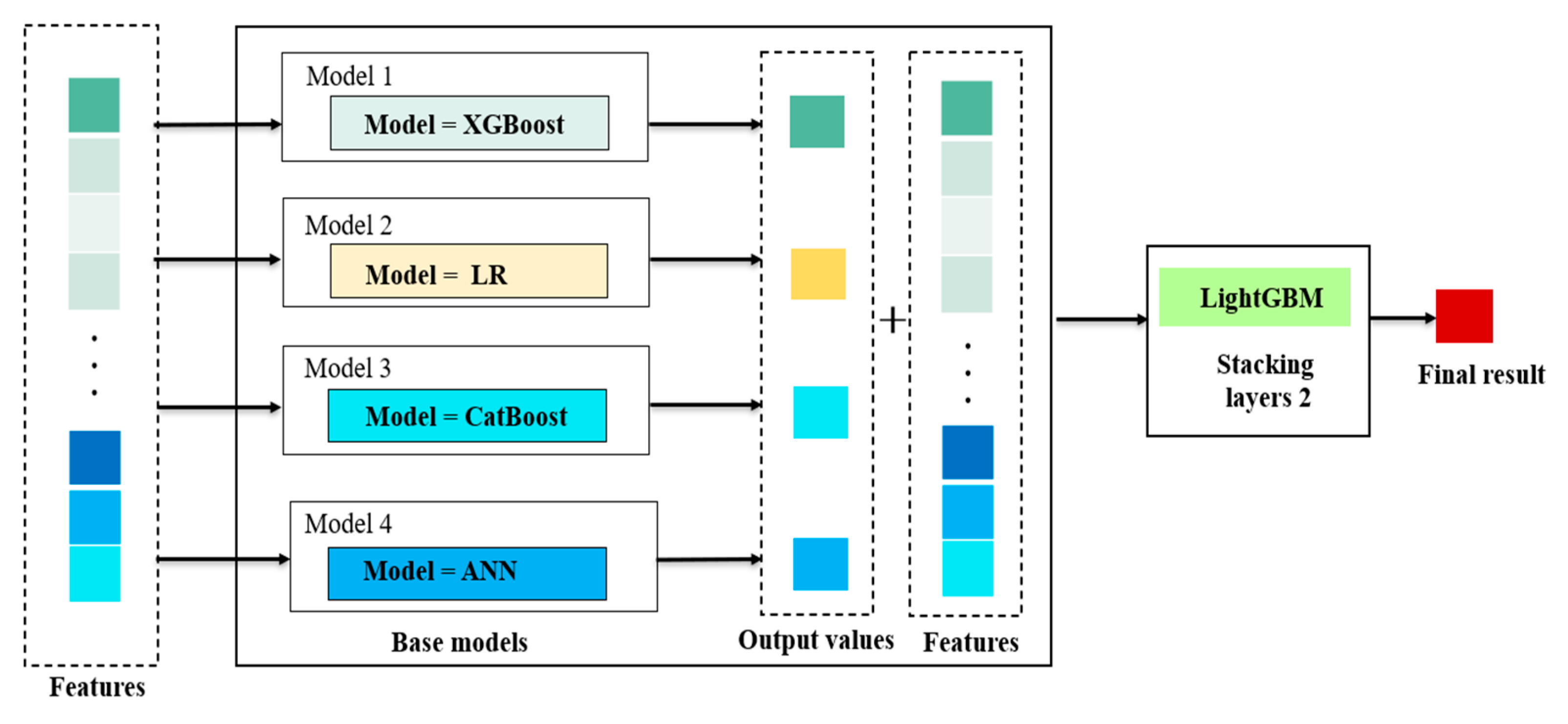
Stacking method is an ensemble machine learning algorithm which can use meta-learning algorithms to learn how to combine the predictions from some base models best. It mainly trains a new model by taking the output of multiple weak learners as input. Based on the stacking, we established a combined model with LR, XGBoost, CatBoost, and ANN as the base models and LightGBM as the meta model, as shown in Figure 1.

Figure 1.
Ensemble Model by Stacking. Note: Features in Figure 1 are the characteristic variables of the respondents in the CGSS sample. Models 1–4 are the base models. Output values are prediction results of the underlying model. LightGBM is in the second layer of the stacking model, which is the meta model.
In our stacking model, the features affecting residents’ SWB from the CGSS data are put into the traditional statistical model LR and the machine learning models—XGBoost, CatBoost and ANN. Then the predictions of these four models and the original features are put into the LightGBM model. The output results of LightGBM are the basis for judging residents’ SWB. The models selected above obey different principles when fitting datasets and have their own advantages in dealing with various types of variables. For the base models, LR has a strong stability and interpretability. The XGBoost model adds a regular term to control the complexity of the model, which can effectively improve the prediction accuracy of the model. CatBoost can deal with the classification features more efficiently and reasonably, which has solved the problems of gradient deviation and prediction migration and thus reduces the probability of overfitting. ANN has great advantages in dealing with random data and nonlinear data, especially for the large-scale, complex structure and unclear information datasets. For the meta model, LightGBM uses a one-sided gradient algorithm to filter out the samples with small gradients, which reduces the unnecessary calculating and computing. It also uses the optimized features to accelerate parallel calculation. The stacking model can extract more information from these models and combine all these advantages to achieve a good performance on forecasting. Therefore, when selecting models for stacking, we tried to choose models with different fitting principles if possible.
3.2. The Evaluation Index of a Model
Due to the imbalance of datasets, we used over-sampling and under-sampling methods to make the ratio of positive and negative samples at 1:1. Moreover, the ratio of the training set and test set was divided into 8:2. The model evaluation indexes were as follows [37,38].
- (1)
- Accuracy, precision, and F1 score. In the binary classification algorithm model, accuracy is the proportion of all accurate classifications to the number of all samples. Precision is the proportion of positive samples correctly predicted out of all samples predicted as positive. Recall is the proportion of positive samples correctly predicted out of all the positive samples. The F1 score is the harmonic average of precision and recall.
- (2)
- AUC (Area Under ROC Curve) value is a number that ranges from 0 to 1, which measures the area under the ROC (Receiver Operating Characteristic) curve. The higher the AUC value obtained, the better the classification model performs.
- (3)
- KS (Kolmogrov–Smirnov) value represents the ability of the model to segment samples. The greater the KS value is, the stronger the ability.
3.3. Datasets and Features
The data we adopted in this paper were from CGSS, hosted by the National Survey Research Center at Renmin University of China. It collects representative samples of all urban and rural households in 31 provinces/autonomous regions/municipalities (excluding Hong Kong, Macao, and Taiwan) of China, using the multi-stage, hierarchical and PPS (Probability Proportionate to Size Sampling) random sampling methods. The CGSS2011, CGSS2013, CGSS2015, and CGSS2017 datasets used in this paper are samples collected from 100 county-level units plus 5 metropolises, 480 communities (village/neighborhood committees), and 12000 families in China every year. Take CGSS2015 as example. In the preprocessing stage, we took a36 (level of happiness) as the proxy variable for SWB. In the survey, the relevant question was: “Generally speaking, how happy do you feel about your life?” Possible responses included: “totally unhappy”, “a little unhappy”, “neither happy nor unhappy”, “generally happy”, “completely happy”. To simplify the classification, “neither happy nor unhappy”, “generally happy” and “completely happy” were merged as “happy”, and noted as “1”. While “totally unhappy” and “a little unhappy” were merged as “unhappy”, and noted as “0”. Then we deleted the unrelated features in the data and filled the missing values with average values. To extract more effective information and improve prediction accuracy, feature engineering methods were used to add, filter, and merge the original features. The description and measures of the new features are shown in Table 1.

Table 1.
Method and explanation of feature engineering.
3.4. Empirical Process
For the data preprocessing, we first deleted the features unrelated to SWB and constructed some new features. Second, we used the over-sampling and under-sampling methods to balance the ratio of the positive and negative samples. Third, the samples were divided into a training set and a test set at 8:2. Then the balanced data was put into the traditional statistical model, the machine learning model, and the stacking model, respectively.
On the model fitting for the machine learning models, a k-fold cross-validation method was adopted to choose the hyper-parameters and to enhance the robustness and the generalization ability. As shown in Figure 2, we divided the original training data into five equally sized parts (named folds). During the 5 iterations, 4 folds were used for training, while the other 1 fold was used as the test set for the model evaluation. Then, the estimated performance (such as classification accuracy) for each fold was used to calculate the estimated average performance S of the model. By using this cross-validation method, the hyper-parameters of the base models were tuned with the training and validation subsets. After tuning, we trained the base models with the best hyper-parameters and at last, the performance of the best base models was tested in the test subset.
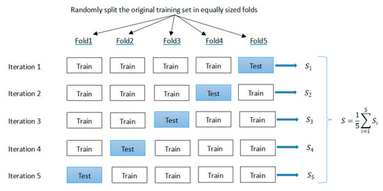
Figure 2.
The figure of k-fold cross-validation.
After adjusting the parameters and analyzing the importance of the features, we compared the results of the base models with the stacking model. Then the common factors that affect SWB across years were obtained.
4. Results
4.1. SWB Prediction Based on Single Models
LR, XGBoost, CatBoost, LightGBM, ANN, and CNN are established in this section, and 5-fold cross-validation is used on the training set to tune their hyper-parameters, respectively (Parameter regulation results can be requested from the author).
4.1.1. LR
Evaluations results based on LR are shown in Table 2.
Table 2.
Evaluation results based on LR.
Evaluations results based on LR, especially the AUC value were used as references to compare with the other models.
4.1.2. XGBoost
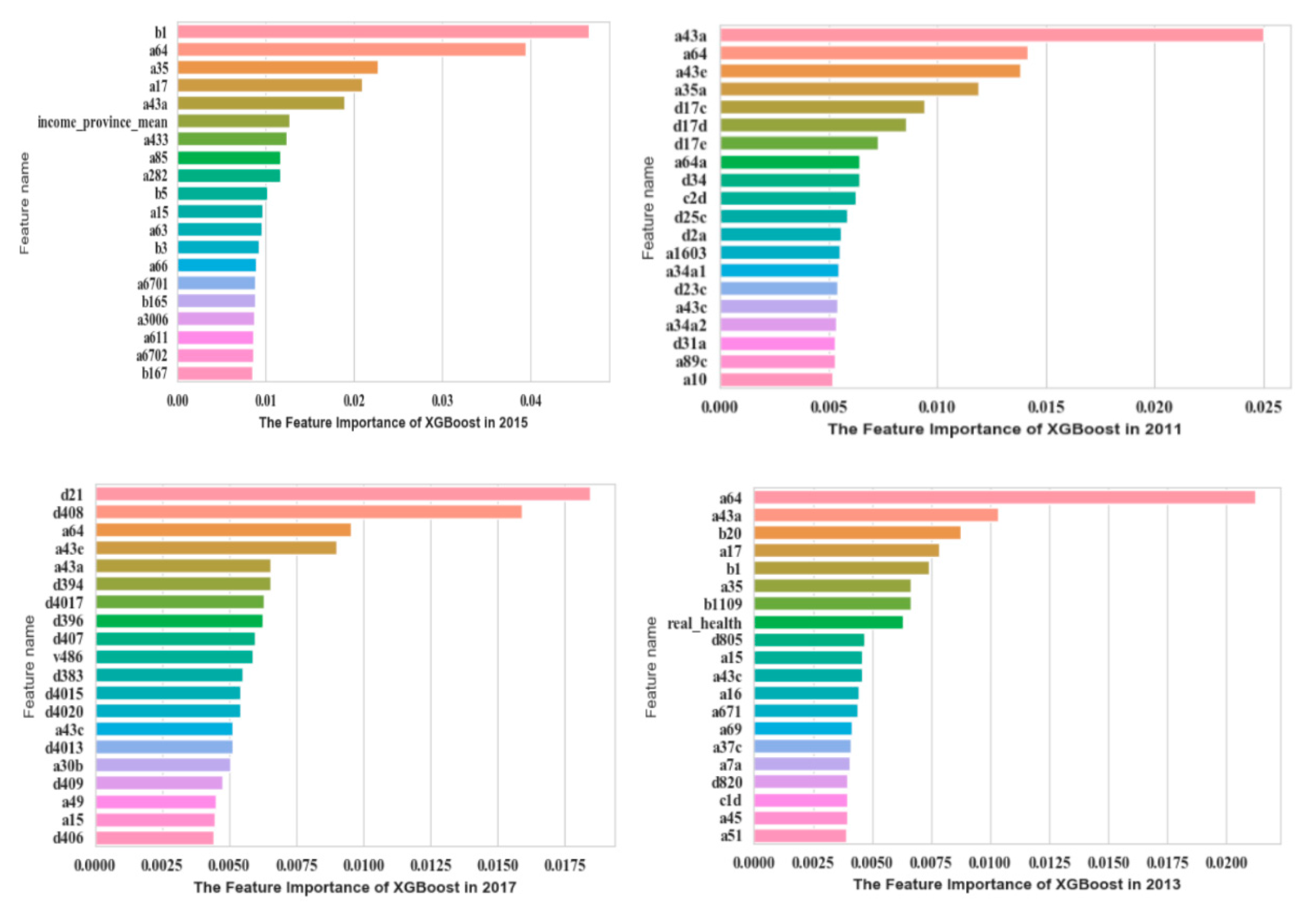
The XGBoost model was established to improve the prediction accuracy. Then we gained the top 20 significant features from the CGSS data. A detailed description is shown in Figure 3.

Figure 3.
Top 20 significant features of CGSS based on XGBoost.
In CGSS2011, a43a (self-perceived social class at present), a64 (family economic status), and a43e (self-perceived social class compared to contemporary) were much more significant. Then in CGSS2013, the importance of features such as a64 (family economic status), a43a (self-perceived social class at present), and b20 (the living conditions compared with ordinary people) ranked higher. In 2015CGSS, b1 (social and economic status compared with peers), a64 (family economic status), and a35 (self-perceived social equity) were the features that contributed the most to SWB. In CGSS2017, features such as d21 (satisfaction with current living conditions), d408 (satisfaction of family’s income), a64 (family economic status), and a43e (self-perceived social class compared to contemporary) ranked higher in importance. It can be judged that these features have a significant influence on SWB.
The evaluation results of the XGBoost are shown in Table 3. The AUC of XGBoost established from the data from 2011, 2013, 2015, and 2017 were better than LR.
Table 3.
Evaluation results based on XGBoost.
4.1.3. CatBoost
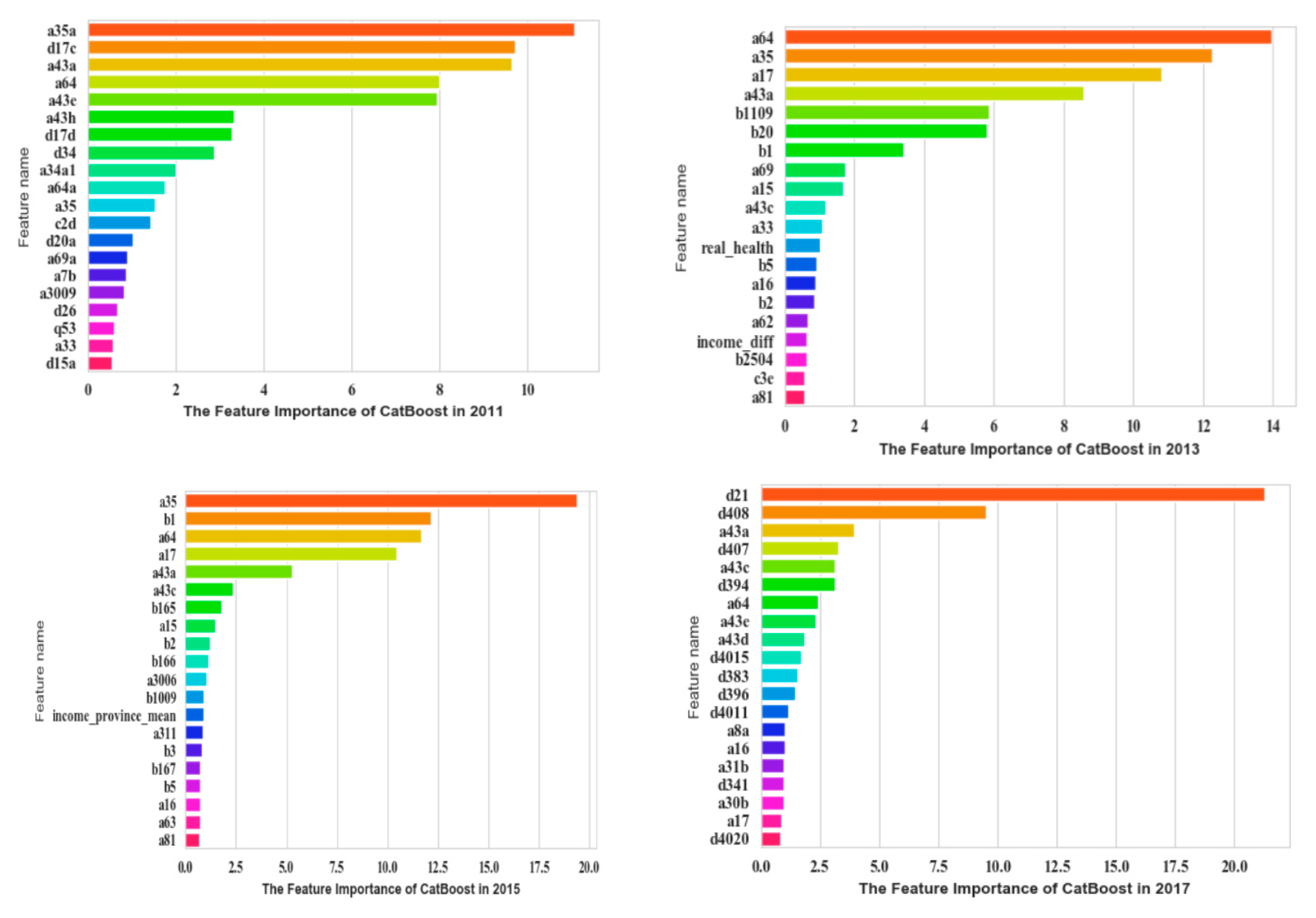
The most significant 20 features were obtained based on CatBoost, which are shown in Figure 4.

Figure 4.
Top 20 significant features of CGSS based on CatBoost.
In CGSS2011, a35a (fairness of current living standard compared with your efforts), d17c (frequency of depression in the past four weeks), a43a (self-perceived social class at present), and a64 (family economic status) ranked higher. In CGSS2013, a64 (family economic status), a35 (self-perceived social equity), a17 (frequency of depression in the past four weeks), and a43a (self-perceived social class at present) ranked higher. In CGSS2015, a35 (self-perceived social equity), b1 (social and economic status compared with peers), a64 (family economic status), and a17 (frequency of depression in the past four weeks) ranked higher. In CGSS2017 d21 (satisfaction with current living conditions), d408 (satisfaction of family’s income), a43a (self-perceived social class at present), and d407 (self-sufficiency compared with people around) ranked higher. The evaluation indexes of the model are shown in Table 4.
Table 4.
Evaluation results based on CatBoost.
4.1.4. LightGBM
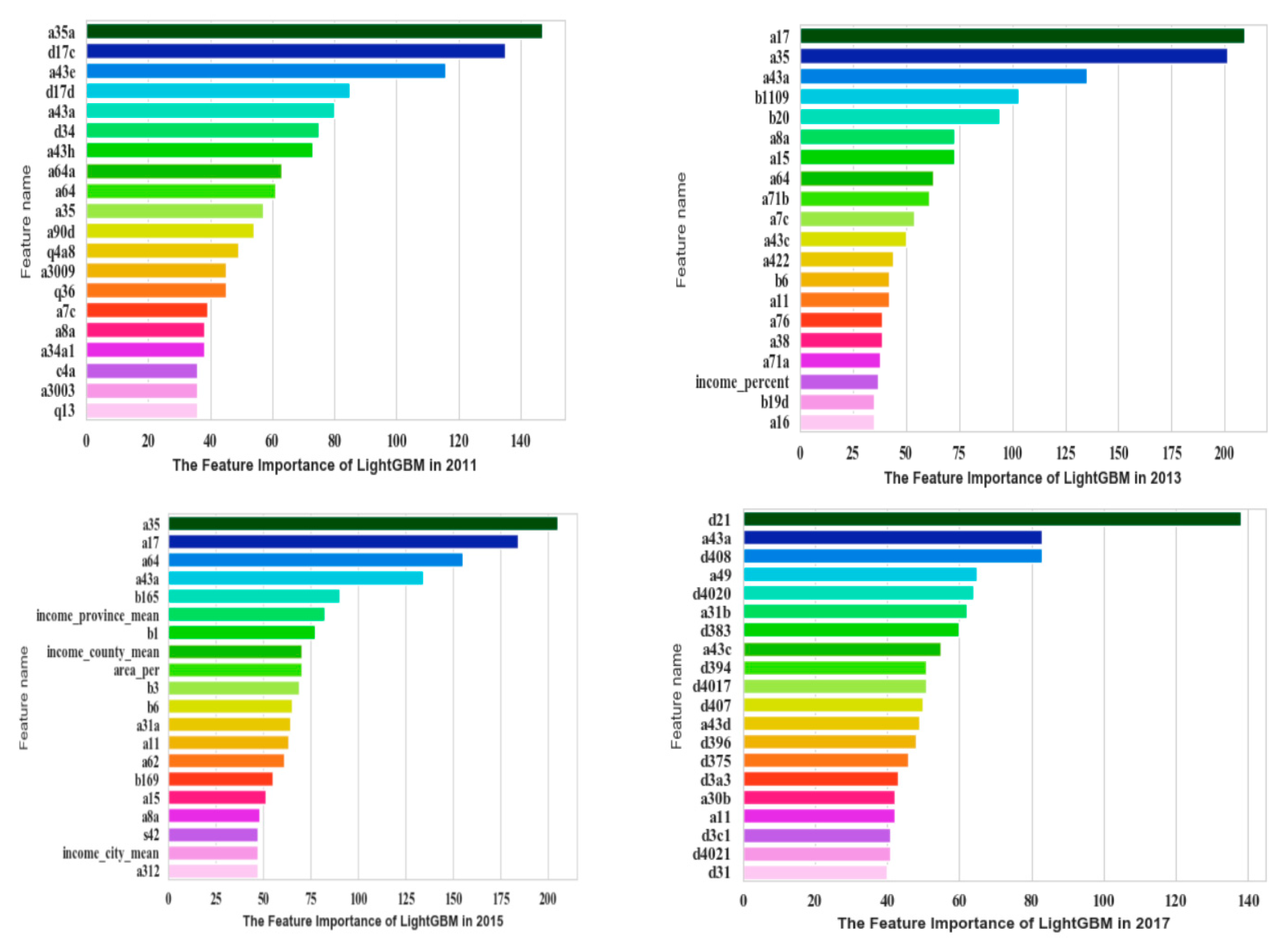
The most important 20 features based on LightGBM are shown in Figure 5.
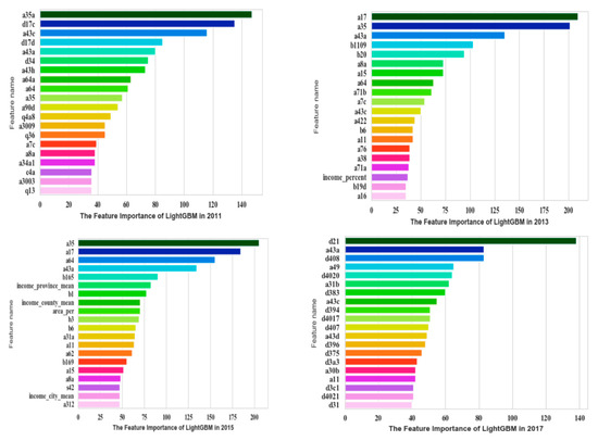
Figure 5.
Top 20 important features of CGSS based on LightGBM.
In CGSS2011, a35a (fairness of current living standard compared with your effort), d17c (frequency of depression in the past four weeks), and a43e (self-perceived social class compared to contemporary) were the most significant features. In CGSS2013, a17 (frequency of depression in the past four weeks), a35 (self-perceived social equity), and a43a (self-perceived social class at present) were the most significant features. In CGSS2015, a35 (self-perceived social equity), a17 (frequency of depression in the past four weeks), a64 (family economic status), and a43a (self-perceived social class at present) were the most significant features. In CGSS2017, d21 (satisfaction with current living conditions), a43a (self-perceived social class at present), d408 (satisfaction of family’s income), and a49 (ability to understand Mandarin) were the most significant features. Table 5 shows the evaluation results of the LightGBM.
Table 5.
Evaluation results based on LightGBM.
4.1.5. ANN
Evaluation results based on ANN are shown in Table 6.
Table 6.
Evaluation results based on ANN.
Evaluations results based on ANN, especially the AUC values were used as references to compare with the other models.
4.1.6. CNN
As a kind of feed-forward neural network, CNN can automatically extract features from its convolution layer to complete the work of model optimization. The evaluation results of the CNN are shown in Table 7.
Table 7.
Evaluation results based on CNN.
Evaluations results based on CNN, especially the AUC value were used as references to compare with the other models.
4.2. SWB Prediction Based on a Stacking Model
To improve the performance of the base models, we proposed a stacking model, combining machine learning and LR to enhance the forecasting process. In this model, LR, XGBoost, CatBoost, and ANN were used as the base models, and LightGBM was used as the meta model to predict the SWB of residents.
With the AUC index, the performance of the stacking model and the single model is shown in Table 8. Compared with the traditional LR model, the AUC value of the stacking model increased by 15.37% in 2017. Compared with other machine learning models, the stacking model is still better, including XGBoost, CatBoost, LightGBM, ANN, and the current popular deep learning model CNN.
Table 8.
AUC values of the single and stacking models.
After considering the classification performance of the stacking model and the single model, the running time of the above models were analyzed. This was computed by putting the target data into the predicting models. The running time is shown in Table 9.
Table 9.
Running time (s) of the single and stacking models.
As shown in Table 9, the LR model had the shortest running time, but the prediction accuracy was low; the CNN model, due to its multiple convolutional layers and pooling layers, had too long a running time to be suitable for real-time detection. Compared with these tree-based single models, the XGBoost model had almost twice the time of the stacking model. Although the running times of CatBoost, LightGBM, and ANN were similar to the stacking model, it can be seen in Table 8 that their prediction accuracy was generally lower. In terms of the classification results and running time, it can be comprehensively stated that the stacking model proposed in this paper has a short running time while achieving the best classification performance.
When selecting the meta model, we compared the performance of the stacking model based on LightGBM, LR, XGBoost, CatBoost, and ANN, respectively. The results are shown in Table 10.
Table 10.
The AUC value of the stacking model based on different meta models.
4.3. Statistical Analysis
In the above experiments, five indicators were used to evaluate the prediction accuracy and prediction ability of the model, but it was still necessary to indicate whether the differences in models’ performance were statistically significant or not. The Friedman test and the Nemenyi test were used to verify the results.
The Friedman test compares the average ranks of algorithms, , where is the rank of the j-th of k algorithms on the i-th of N datasets. In our experiment, there were seven models and four years of datasets, which means N = 4 and k = 7. The average ranks were assigned by sorting the AUC values of the models from good to bad. The null hypothesis of the Friedman test is that all the models are equivalent. The Friedman statistic is distributed according to the F distribution with k − 1 and (k − 1)(N − 1) degrees of freedom, as shown in the following equation [39],
The value of the was 15.1621 and its p-value was 0.0183. Since the p-value was less than 0.05, this indicates that the hypothesis test rejected the null hypothesis and the performance of the model was significantly different.
However, the Friedman test can only show that there is a difference between the accuracy of the models; it cannot distinguish the differences more accurately. Therefore, the Nemenyi test was needed to further verify whether there was a significant difference in the accuracy between the seven models. In the Nemenyi test, the CD (the corresponding average ranks differ by at least the critical difference) values can be calculated by the following formula [39]:
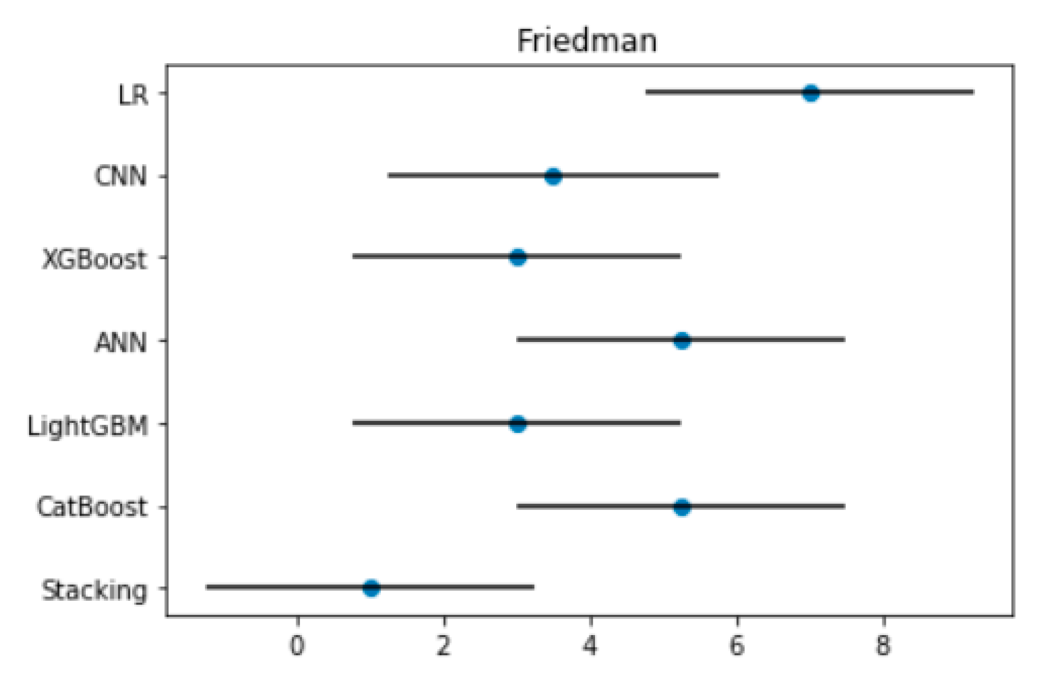
where can be obtained from Demšar J.’s related work. According to the calculation, the is 2.949 at the significance level of α = 0.05 in the paper and the CD is equal to 4.50. This indicates that if the difference of any two models’ average ranks is greater than 4.50, there is a significant difference in performance of the two models. Furthermore, the results of the Friedman test and Nemenyi test can be visually represented in Figure 6.
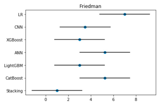
Figure 6.
The figure of the Friedman test. Note: The ordinate in the figure represents the seven models, the horizontal axis represents the average rank value; the solid circle represents the average rank value corresponding to the model; the horizontal line represents the size of the CD.
As shown in Figure 6, there was almost no overlap between the horizontal line segments of the Stacking model and the CatBoost, ANN, and LR models. Therefore, it can be considered that there was a significant difference between these models. The Stacking model and the LightGBM, XGBoost, and CNN models partially overlapped, indicating that the performance of these models had a certain similarity from the perspective of statistical testing.
5. Discussion
This paper has proposed a stacking model with LR, XGBoost, CatBoost, and ANN as the base models and LightGBM as the meta model. Based on data from different years, the stacking model has a good effect on the SWB forecasting. The results show that the stacking model we constructed could learn more information from the same data samples and improve the accuracy by integrating the advantages of different base models. The results prove the applicability of the stacking algorithm on the SWB forecasting tasks.
Nevertheless, we also compared the top 20 features of annual samples (excluding the input variables of the base model in stacking) in the stacking model. Table 11 shows the similar features of each year.
Table 11.
Similar features affecting SWB in different years.
According to Table 11, one of the common significant features of 2011, 2013, and 2015 was the degree of the respondents’ self-perceived social equity (a43e, a35), but the importance of the feature was no longer prominent in 2017. To some extent, the equity and justice in society that Chinese residents have pursued have been realized during the development of the country. It also reveals that the concept of equity has been gradually established in the society. The Chinese government has guided people to establish a dialectical concept of equity, to treat society rationally, and to treat themselves correctly. Under this circumstance, the Chinese people persist in creating happy lives through hard work. Further, through deepening structural reform, China has gradually achieved equity in many areas of society and has improved the sense of social justice and the SWB of citizens.
As another important feature of SWB in 2011 and 2013, respondents’ annual income was not reflected in 2015 and 2017, which means that the influence of total income has gradually decreased as time passed. This result shows that, with the modernization and development of China, the income level of residents has been greatly improved. The absolute income is no longer the only dominant factor affecting SWB.
Furthermore, it is noticeable that there were several important factors which were not related to income in 2011, 2013, 2015, and 2017. In 2011, there were features such as respondents’ self-perceived social class, degree of freedom, and frequency of depression. In 2013, there were features such as self-perceived social class, degree of comfort, and frequency of depression. In 2015, there were features such as respondents’ satisfaction with employment. In 2017, there were features such as the respondents’ self-perceived social class, frequency of social entertainment, and satisfaction of current living conditions. With the continuous development of the economy and society, people’s desire for a better life is becoming much stronger. The demand from people has changed from material wealth to the spiritual aspect, from satisfaction in relation to material quantity to the pursuit of quality of life. Therefore, enriching the demand of people’s spiritual and cultural life, promoting the construction of spiritual civilization, and enhancing people’s sense of security, acquisition as well as happiness will be the direction of further reform and development over a long period.
6. Conclusions
To improve the performance of predicting the SWB of residents and explore the determinant factors, we conduct an empirical analysis based on CGSS2011, CGSS2013, CGSS2015, and CGSS2017 data.
Six machine learning and deep learning algorithms are selected, namely LR, XGBoost, CatBoost, LightGBM, ANN, and CNN. A stacking model is constructed by taking the ANN, XGBoost, LR, and CatBoost as the base models, while the LightGBM is taken as the meta model. With the over-sampling and under-sampling method, we obtain 20 important features which are highly correlated to the SWB of residents. The similarities and differences among these features in 4 years are beneficial for studying what factors influence the SWB of residents the most. The results show that machine learning models can generally achieves a better forecasting accuracy than the traditional LR, while the stacking model achieved the best performance among all the algorithms. Meanwhile, the Friedman test and the Nemenyi test are used to verify the experimental results, indicating that the difference in performance of models is statistically significant.
For the features that affect the SWB of residents in different years, this paper has extracted the top 20 related features. For further research, the scope of influencing features can be expanded to analyze the differences and connections between various features, which will be beneficial for improving the forecasting performance of SWB.
Author Contributions
Conceptualization, N.K., G.S. and Y.Z.; data curation, N.K. and Y.Z.; methodology, N.K. and G.S.; software, N.K. and Y.Z.; visualization, Y.Z.; writing—original draft, N.K., Y.Z. and G.S.; writing—review and editing, N.K. and G.S.; project administration, G.S.; funding acquisition, G.S. All authors have read and agreed to the published version of the manuscript.
Funding
This research was supported by the National Funds of Social Science (China, grant number 13&ZD172).
Institutional Review Board Statement
Not applicable.
Informed Consent Statement
Not applicable.
Data Availability Statement
Publicly available datasets were analyzed in this study. This data can be found here: http://cnsda.ruc.edu.cn/index.php?r=site/datarecommendation, accessed on 30 August 2021.
Conflicts of Interest
The authors declare no conflict of interest.
Abbreviations
| SWB | Subjective Well-Being |
| CGSS | Chinese General Social Survey |
| LR | Logistic Regression |
| SES | Socio-economic Status |
| SVM | Support Vector Machine |
| DT | Decision Tree |
| KNN | K-Nearest Neighbor |
| GBDT | Gradient Boosting Decision Tree |
| XGBoost | Extreme Gradient Boosting |
| LightGBM | Light Gradient Boosting Machine |
| Catboost | Category Boosting |
| ANN | Artificial Neural Network |
| CNN | Convolutional Neural Network |
| MLR | Multiple Linear Regression |
| ROC | Receiver Operating Characteristic |
| AUC | Area Under ROC Curve |
| KS | Kolmogrov-Smirnov |
| BMI | Body Mass Index |
References
- Wilson, W.R. Correlates of avowed happiness. Psychol. Bull. 1967, 67, 294–306. [Google Scholar] [CrossRef]
- Diener, E. The Science of Well-Being; Springer: Dordrecht, The Netherlands, 2009. [Google Scholar] [CrossRef]
- Diener, E.; Suh, E.M.; Lucas, R.E.; Smith, H.L. Subjective well-being: Three decades of progress. Psychol. Bull. 1999, 125, 276–302. [Google Scholar] [CrossRef]
- Diener, E.; Oishi, S.; Tay, L. Advances in subjective well-being research. Nat. Hum. Behav. 2018, 2, 253–260. [Google Scholar] [CrossRef] [PubMed]
- Yang, Q.; Cheng, C.; Zhang, K. Income Gap, Housing Property Rights and the Urban Residents’ Happiness: Based on Empirical Research of CGSS2003 and CGSS2013. Northwest Popul. J. 2018, 39, 11–29. (In Chinese) [Google Scholar]
- Ferrer-I-Carbonell, A.; Gowdy, J.M. Environmental degradation and happiness. Ecol. Econ. 2007, 60, 509–516. [Google Scholar] [CrossRef]
- Zhang, N.; Liu, C.; Chen, Z.; An, L.; Ren, D.; Yuan, F.; Yuan, R.; Ji, L.; Bi, Y.; Guo, Z.; et al. Prediction of adolescent subjective well-being: A machine learning approach. Gen. Psychiatry 2019, 32, e100096. [Google Scholar] [CrossRef] [PubMed]
- Chinese National Survey Data Archive. Available online: http://cnsda.ruc.edu.cn/index.php?r=site/datarecommendation (accessed on 4 January 2021).
- Voukelatou, V.; Gabrielli, L.; Miliou, I.; Cresci, S.; Sharma, R.; Tesconi, M.; Pappalardo, L. Measuring objective and subjective well-being: Dimensions and data sources. Int. J. Data Sci. Anal. 2020, 11, 279–309. [Google Scholar] [CrossRef]
- Veenhoven, R. Happiness: Also Known as “Life Satisfaction” and “Subjective Well-Being”. In Handbook of Social Indicators and Quality of Life Research; Land, K., Michalos, A., Sirgy, M., Eds.; Springer: Dordrecht, The Netherlands, 2012. [Google Scholar] [CrossRef] [Green Version]
- Shi, H.; Yi, M. Environmental Governance, High-quality Development and Residents’ Happiness—Empirical Study Based on CGSS (2015) Micro Survey Data. Manag. Rev. 2020, 32, 18–33. (In Chinese) [Google Scholar]
- Pan, H.; Chen, H. Empirical Research on the Effect Mechanism of Ecological Environment on Residents’ Happiness in China. Chin. J. Environ. Manag. 2021, 13, 156–161, 148. (In Chinese) [Google Scholar]
- Clark, A.E.; Frijters, P.; Shields, M.A. Relative Income, Happiness, and Utility: An Explanation for the Easterlin Paradox and Other Puzzles. J. Econ. Lit. 2008, 46, 95–144. [Google Scholar] [CrossRef] [Green Version]
- Esping-Andersen, G.; Nedoluzhko, L. Inequality equilibria and individual well-being. Soc. Sci. Res. 2017, 62, 24–28. [Google Scholar] [CrossRef]
- Johnson, W.; Krueger, R.F. How money buys happiness: Genetic and environmental processes linking finances and life satisfaction. J. Pers. Soc. Psychol. 2006, 90, 680–691. [Google Scholar] [CrossRef]
- Tan, J.J.X.; Kraus, M.W.; Carpenter, N.C.; Adler, N.E. The association between objective and subjective socioeconomic status and subjective well-being: A meta-analytic review. Psychol. Bull. 2020, 146, 970–1020. [Google Scholar] [CrossRef]
- Molina, M.; Garip, F. Machine Learning for Sociology. Annu. Rev. Sociol. 2019, 45, 27–45. [Google Scholar] [CrossRef] [Green Version]
- Samuel, A.L. Some Studies in Machine Learning Using the Game of Checkers. IBM J. Res. Dev. 1959, 3, 210–229. [Google Scholar] [CrossRef]
- Kotsiantis, S.B.; Zaharakis, I.; Pintelas, P. Supervised machine learning: A review of classification techniques. Emerg. Artif. Intell. Appl. Comput. Eng. 2007, 160, 3–24. [Google Scholar]
- Saputri, T.R.D.; Lee, S.-W. A Study of Cross-National Differences in Happiness Factors Using Machine Learning Approach. Int. J. Softw. Eng. Knowl. Eng. 2015, 25, 1699–1702. [Google Scholar] [CrossRef]
- Jaques, N.; Taylor, S.; Azaria, A.; Ghandeharioun, A.; Sano, A.; Picard, R. Predicting students’ happiness from physiology, phone, mobility, and behavioral data. In Proceedings of the 2015 International Conference on Affective Computing and Intelligent Interaction (ACII), Xi’an, China, 21–24 September 2015; pp. 222–228. [Google Scholar] [CrossRef] [Green Version]
- Marinucci, A.; Kraska, J.; Costello, S. Recreating the Relationship between Subjective Wellbeing and Personality Using Machine Learning: An Investigation into Facebook Online Behaviours. Big Data Cogn. Comput. 2018, 2, 29. [Google Scholar] [CrossRef] [Green Version]
- Dietterich, T.G. Ensemble Methods in Machine Learning; Springer: Berlin/Heidelberg, Germany, 2000; pp. 1–15. [Google Scholar] [CrossRef] [Green Version]
- Breiman, L. Bagging predictors. Mach. Learn. 1996, 24, 123–140. [Google Scholar] [CrossRef] [Green Version]
- Zhang, Z.L.; Wu, D.P. An imbalanced data classification method based on probability threshold Bagging. Comput. Eng. Sci. 2019, 41, 1086–1094. (In Chinese) [Google Scholar]
- Tuysuzoglu, G.; Birant, D. Enhanced Bagging (eBagging): A Novel Approach for Ensemble Learning. Int. Arab. J. Inf. Technol. 2019, 17, 515–528. [Google Scholar]
- Friedman, J.H. Greedy function approximation: A gradient boosting machine. Ann. Stat. 2001, 29, 1189–1232. [Google Scholar] [CrossRef]
- Chen, T.; Guestrin, C. XGBoost: A Scalable Tree Boosting System. In Proceedings of the 22nd ACM SIGKDD International Conference on Knowledge Discovery and Data Mining, San Francisco, CA, USA, 13–17 August 2016; pp. 785–794. [Google Scholar] [CrossRef] [Green Version]
- Ke, G.; Meng, Q.; Finley, T.; Wang, T.; Chen, W.; Ma, W.; Ye, Q.; Liu, T.-Y. LightGBM: A Highly Efficient Gradient Boosting Decision Tree. In Proceedings of the 31st Conference on Neural Information Processing Systems (NIPS 2017), Long Beach, CA, USA, 4–9 December 2017. [Google Scholar]
- Prokhorenkova, L.; Gusev, G.; Vorobev, A.; Dorogush, A.V.; Gulin, A. CatBoost: Unbiased boosting with categorical features. Adv. Neural Inf. Process. Syst. 2018, 31, 6639–6649. [Google Scholar]
- Wolpert, D.H. Stacked generalization. Neural Netw. 1992, 5, 241–259. [Google Scholar] [CrossRef]
- Ting, K.M.; Witten, I. Issues in Stacked Generalization. J. Artif. Intell. Res. 1999, 10, 271–289. [Google Scholar] [CrossRef] [Green Version]
- Sigletos, G.; Paliouras, G.; Spyropoulos, C.D.; Hatzopoulos, M. Combining Information Extraction Systems Using Voting and Stacked Generalization. J. Mach. Learn. Res. 2005, 6, 1751–1782. [Google Scholar]
- Cao, Z.; Yu, D.; Shi, J.; Zong, S. The Two-layer Classifier Model and its Application to Personal Credit Assessment. Control. Eng. China 2019, 26, 2231–2234. (In Chinese) [Google Scholar]
- McCulloch, W.S.; Pitts, W. A logical calculus of the ideas immanent in nervous activity. Bull. Math. Biol. 1943, 5, 115–133. [Google Scholar] [CrossRef]
- Egilmez, G.; Erdil, N.; Arani, O.M.; Vahid, M. Application of artificial neural networks to assess student happiness. Int. J. Appl. Decis. Sci. 2019, 12, 115. [Google Scholar] [CrossRef]
- Tharwat, A. Classification assessment methods. Appl. Comput. Inform. 2020, 17, 168–192. [Google Scholar] [CrossRef]
- Li, Y.; Chen, W. A Comparative Performance Assessment of Ensemble Learning for Credit Scoring. Mathematics 2020, 8, 1756. [Google Scholar] [CrossRef]
- Demšar, J. Statistical comparisons of classifiers over multiple data sets. J. Mach. Learn. Res. 2006, 7, 1–30. [Google Scholar]

Publisher’s Note: MDPI stays neutral with regard to jurisdictional claims in published maps and institutional affiliations. |
© 2021 by the authors. Licensee MDPI, Basel, Switzerland. This article is an open access article distributed under the terms and conditions of the Creative Commons Attribution (CC BY) license (https://creativecommons.org/licenses/by/4.0/).