1. Introduction
Since the creation of stock markets, there have been attempts to predict their movements, and new predictions methodologies have been devised. Since the 2000s, stock market predictions have been made using various machine learning algorithms beyond qualitative and quantitative methods. Research using multiple algorithms such as the hidden Markov model (HMM), artificial neural network (ANN), genetic algorithm (GA), and support vector machine (SVM) or using a combined model for stock market prediction has been conducted [
1,
2,
3]. Recently, due to the development of deep learning technology, studies applying deep learning to financial markets have been actively conducted. Financial market prediction using deep neural networks (DNNs) based on the improvement of PC computational capabilities was first attempted in [
4], and financial market prediction using RNNs suitable for time series data was attempted in [
5]. Since then, studies have shown that LSTM solves the vanishing gradient problem of recurrent neural networks (RNNs) and is more suitable for predicting financial time series [
6,
7].
The Russell 2000 Index, which has been released since 1982 by US investment advisor Frank Russell, is an index that includes 2000 stocks that are among the top 1001 to 3000 stocks based on market capitalization among 10,000 US listed companies. The number of constituent stocks reaches 2000, but the sum of the market caps of all Russell 2000 stocks is only a single digit share of the market caps of all stocks on the New York Stock Exchange. In this light, the Russell 2000 stocks include many small-scale companies with high growth potential. Unlike the Nasdaq 100 Index, which contains large technology stocks of the top 100 companies by market capitalization, the Russell 2000 Index includes stocks from various industries with proportions greater than 10 percent, such as finance, IT, health care, manufacturing, and consumer discretionary goods. A recent study revealed that when the Russell 2000 industry index begins to rise, stocks belonging to the relevant industry in other countries follow the Russell 2000 industry index and enter a trending period [
8]. Based on this empirical result, this study seeks to predict the date when the Russell 2000 index starts to rise by sector.
In this paper, the denoising autoencoder (DAE), long short-term memory (LSTM), and Pettitt’s test are used to predict the rising change points of the Russell 2000 index by industry. First, we use the DAE to remove the noise from Russell 2000 index data and predict future closing prices using LSTM. Then, Pettitt’s test is performed based on the predicted closing prices to detect the change points.
The empirical results show that the model proposed in this paper is good at detecting rising change points for representative industries. The proposed model could predict a change point approximately 7 days before an actual change point date for several industry indices including consumer discretionary, consumer staples, information technology, and health care industries.
Until now, there have been attempts to find change points in past stock price data [
8] or to predict future stock price movements through deep learning. However, no research to date has attempted to predict future stock price change points. Therefore, this study aims to predict future stock price flows through DAE-LSTM and predict the existence and timing of future change points through Pettitt’s test.
The remainder of this study is organized as follows.
Section 2 presents the literature review, and
Section 3 presents the data and methodology used in this paper.
Section 4 describes the empirical study, and
Section 5 presents the conclusions of our study.
2. Literature Review
2.1. Denoising Autoencoder (DAE)
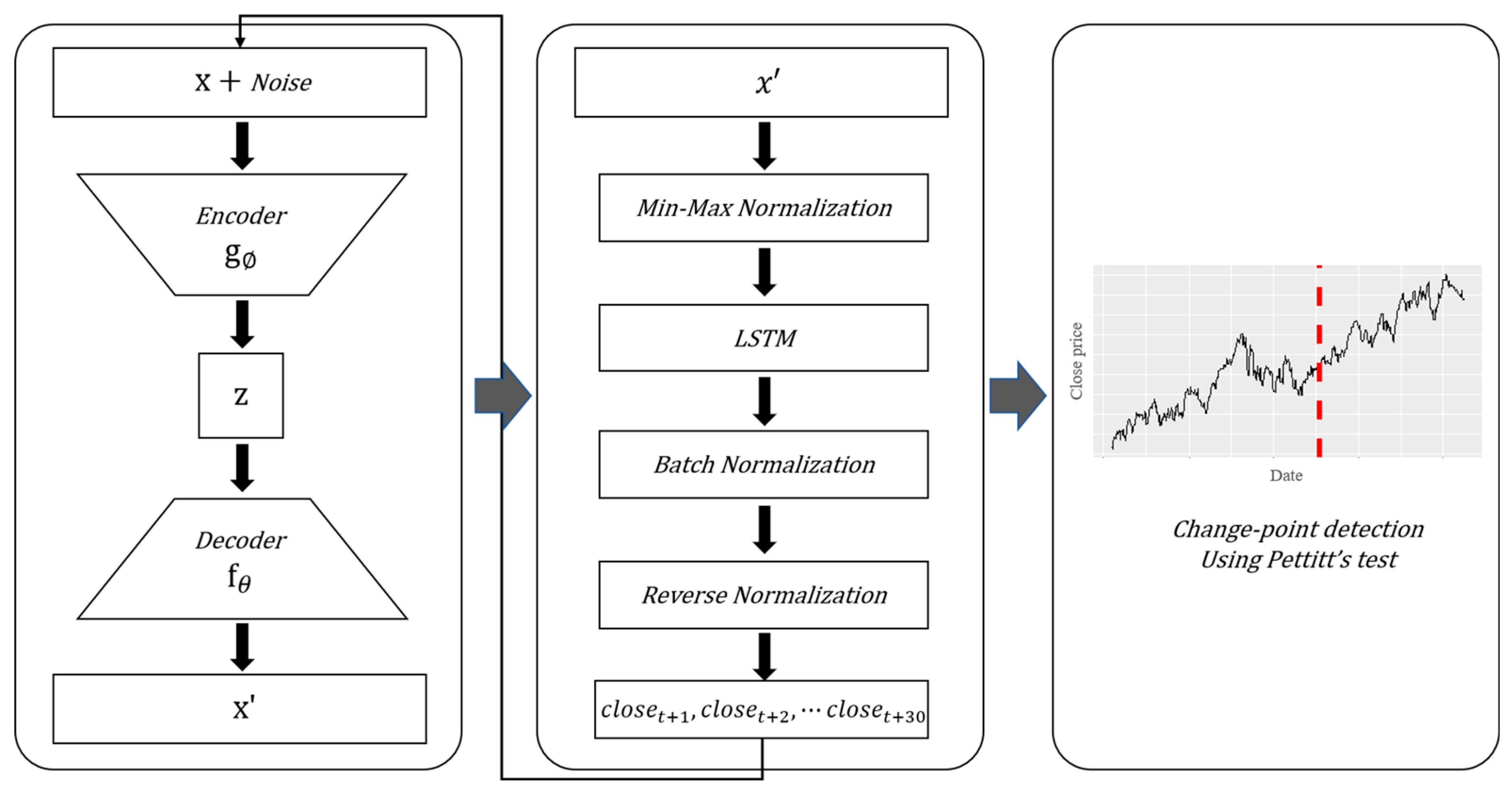
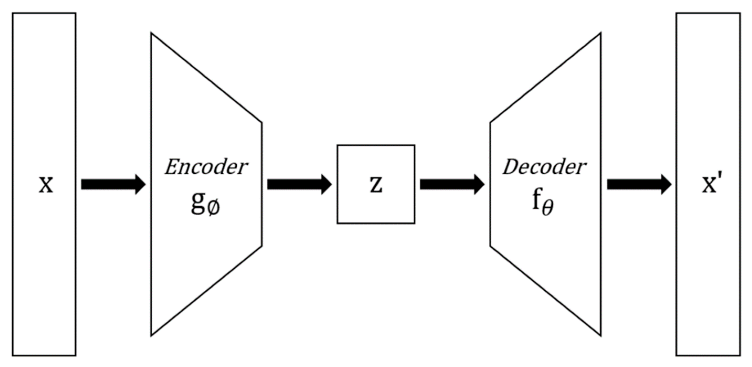
An autoencoder is a type of unsupervised machine learning that learns to approximate an output value to an input value. As shown in
Figure 1, the autoencoder is a neural network structure that consists of an encoder that compresses input data and a decoder that restores the data. In the process of compressing the input data in the encoder, only important information is saved and used as a feature extractor.
The denoising autoencoder, devised by Pascal Vincent [
9], is a model that saves the aforementioned important information and removes the noise of the data by removing the nonessential characteristics. After adding noise to the input data, two methods can be used in the learning process: learning to approximate the data without adding noise and learning by adding dropout to the input. In this study, the model was trained to approximate the original data after adding noise to the input data [
10]. Then, when the data are passed through a neural network that has been trained, noise is removed, and data that retain important features can be obtained.
2.2. Long Short-Term Memory (LSTM)
LSTM is a type of RNN used in deep learning and was designed to solve the vanishing gradient problem, which is a problem in traditional RNNs [
11]. LSTM stores the information of the previous step in a memory cell and determines how much of the past content will be forgotten through the input gate, forget gate, and output gate. The current information is added to the result and delivered to the next point in time.
LSTM networks are suitable for classification, processing, or prediction using time series data. In addition, an advantage of LSTM is that it is insensitive to the length of the input data compared to other algorithms that handle time series data, such as the RNN and HMM. In this study, the tanh function was used as the activation function.
2.3. Pettitt’s Test
Pettitt’s test is a nonparametric test used in several hydroclimatological studies to detect rapid changes in the mean distribution of a variable of interest. This test is based on the Mann–Whitney two-sample test (rank-based test) and can detect a single shift at an unknown time point [
12,
13]. Pettitt’s test, introduced as one of Csorgo and Horvath’s change-point detection methodologies, is defined as follows [
14].
For a series of random variables
two sets of random variables
with the cumulative distribution function
and
with the cumulative distribution function
have a change point at
when
. A test for changes in the distribution uses a nonparametric approach. The alternative hypothesis is established as
, that is, a change point exists; against the null hypothesis
, that is, a change point does not exist. This approach devised by Pettitt [
15] has been applied to detect change points in various continuous data. A test to detect a change point uses the following equations:
The statistic
indicates whether the distributions of the two time series
and
are the same. For
and
at
, Pettitt’s test statistic is defined as follows:
The limiting distribution of
is approximated to
.
2.4. Russell 2000 Index
Managed by FTSE Russell, the Russell 2000 Index was developed in 1984 by the Frank Russell Company. The Russell index is largely divided into three different indices [
16]. These indices are the Russell 1000 index, which consists of the top 1000 stocks by market capitalization; the Russell 2000 index, which consists of the top 1001 to 3000 stocks by market capitalization; and the Russell 3000 index, which consists of the top 3000 stocks by market capitalization. Among these indices, the Russell 2000 index is the most widely used as a small-cap index and the second most used benchmark index after the S&P 500 [
17].
3. Materials and Methodology
The experiment in this study used the daily data of the Russell 2000 sector index from 1 January 2000 to 31 December 2019 provided by Bloomberg. The starting date of the Russell 2000′s trend-up period by industry was used as the starting point of the empirical study [
8].
As shown in
Figure 2, the model proposed in this study is a deep learning combination model for predicting a date when a change point will appear at the present time, and the prediction process is largely composed of three parts. In step 1, after removing the noise from the data through the LSTM stacked denoising autoencoder, LSTM is used to predict the closing price of the next day,
. In step 2, the closing prices of days
,
,…,
are predicted through a moving window model that uses the prediction data generated in step 1 as the input. In step 3, Pettitt’s test is performed with the time series data created in step 2 to find the change points.
3.1. DAE-LSTM-Based Closing Price Prediction Model
In step 1, time point
is determined, and the closing price at time
is predicted using the DAE and LSTM. The autoencoder is trained to approximate the noise-added data to the original data by using 4 years of closing price data as the training dataset and 1 year of closing price data as the validation dataset from the past 5 years of closing price data from time
. We use normally distributed noise at this time following the previous studies that use noise following a normal distribution when they adopt DAE [
18,
19]. Then, the original data are passed through the learned autoencoder to obtain the data from which the nonessential noise has been removed. The denoised data obtained here are used as an input for the LSTM to obtain the closing price at point
.
In the prediction model of step 1, the sequence length when the model is trained and when inputs necessary for prediction are inserted are designated as the five immediately preceding days. All input data are subjected to min–max normalization to improve the learning ability of the model. The final predicted value is calculated by denormalizing the predicted value output through the DAE-LSTM model.
A recent study demonstrated that compared with other machine learning algorithms including multiple linear regression (MLR), support vector regression (SVR), ANN and LSTM, the proposed DAE-LSTM model achieves the best prediction accuracy [
20].
3.2. Repeat the Closing Price Prediction Using LSTM from
to
In this step, the process of predicting the data one point forward is repeated from
to
. At this time, the predicted value of the LSTM model is set to
instead of
to obtain the predicted value of day
, and the predicted value of day
is obtained by setting the predicted value of the model to
. This process is repeated until a predicted value of
is obtained. By repeating this process, the closing price is predicted to obtain a time series predicted from time
to time
.
3.3. Predict Change Points Using Pettitt’s Test
In this step, Pettitt’s test is performed using the predicted time series data obtained through step 1 and step 2 as input data to determine whether there is a change point and to find the date of the change point. Previous studies show that the prediction power in financial markets is improved when the neural network is applied after clustering using the Pettitt’s test [
21,
22]. At this time, if the
p value of Pettitt’s test is less than
, a statistically significant change point is obtained; and if the
p value is greater than
, it can be said that there is no significant change point in the corresponding period.
4. Empirical Study
This study examines four sectors including consumer discretionary (consumer discret), consumer staples, information technology (IT), and health care included in the Russell 2000 index.
Table 1 shows the start date of the rising trend by industry. Only nonoverlapping industries were used among the uptrend days for each industry used in the previous study [
8]. The experiment was conducted using the same process for each industry, and the experiment consisted of three processes.
4.1. Closing Price Prediction Using DAE-LSTM
First, we measured the frequency of change points in the Russell 2000 index by sector. Pettitt’s test was conducted for each sector and period corresponding to the test subject. This period refers to the five-year period before the start of the general trend of each sector. After Pettitt’s test was conducted for the entire period, Pettitt’s test was conducted by dividing the period based on the corresponding change point. This process was repeated until the p value of Pettitt’s test was greater than 0.05 and there was no change point in the corresponding period. The interval of change points was measured and averaged. The average interval of change points based on the 95% confidence level was 25.32 days, and a change point was detected within 30 days. Therefore, 15 days before the start date of the uptrend was set as time
in step 1, and the closing prices from
to
in step 2 were predicted.
The time
set according to the above criteria by sector is as follows.
After dividing the data based on the selected time
t in
Table 2, the noise in the data were removed through the DAE. Five years of daily data before time
t were used. The first 4 years of data were used as the training dataset and the next 1 year of data was used as the validation dataset. In the learning process, the sequence length was set to 5, the learning rate was 0.0001, and the number of learning sessions was set to 10,000. The loss function was the MSE (mean squared error), the optimization function was the Adam optimizer, and batch normalization was used to prevent overfitting during training. The denoised closing price data for each industry were obtained by using the data from the 5 years before point
as input data to the trained model.
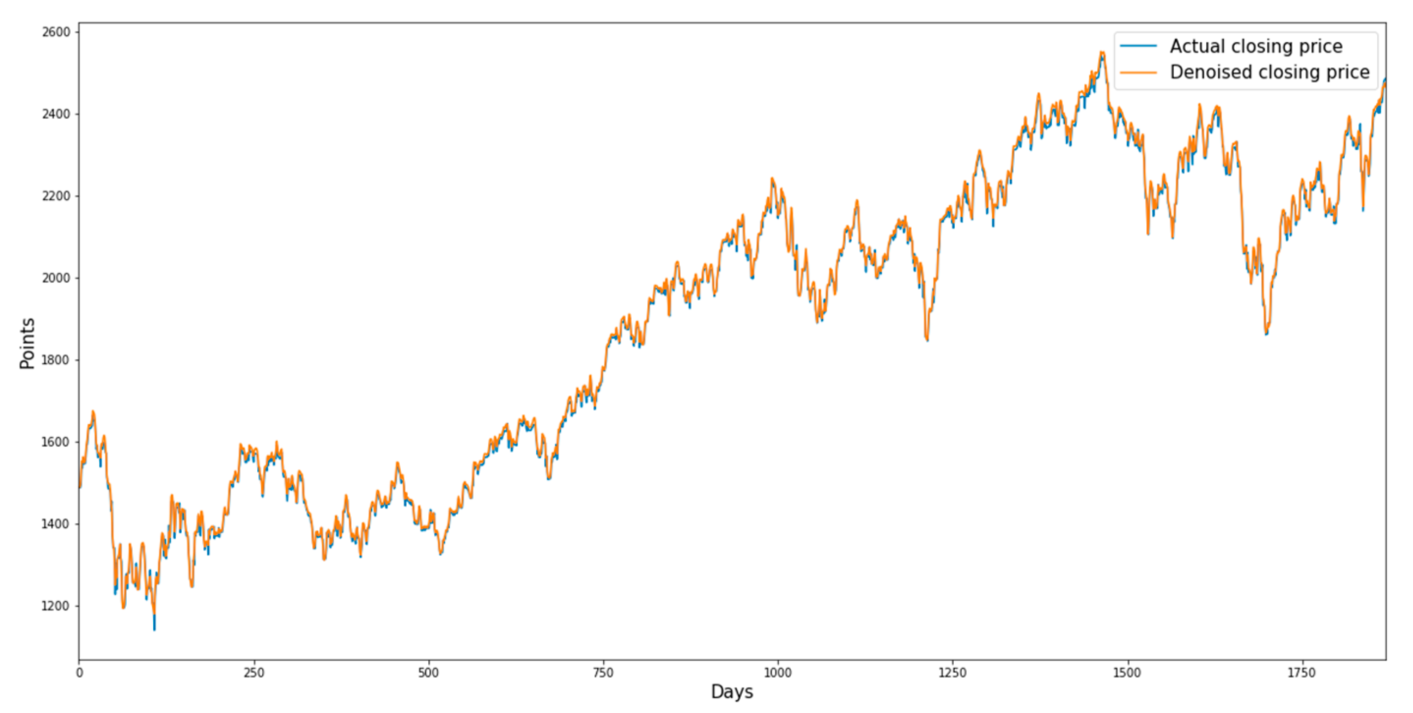
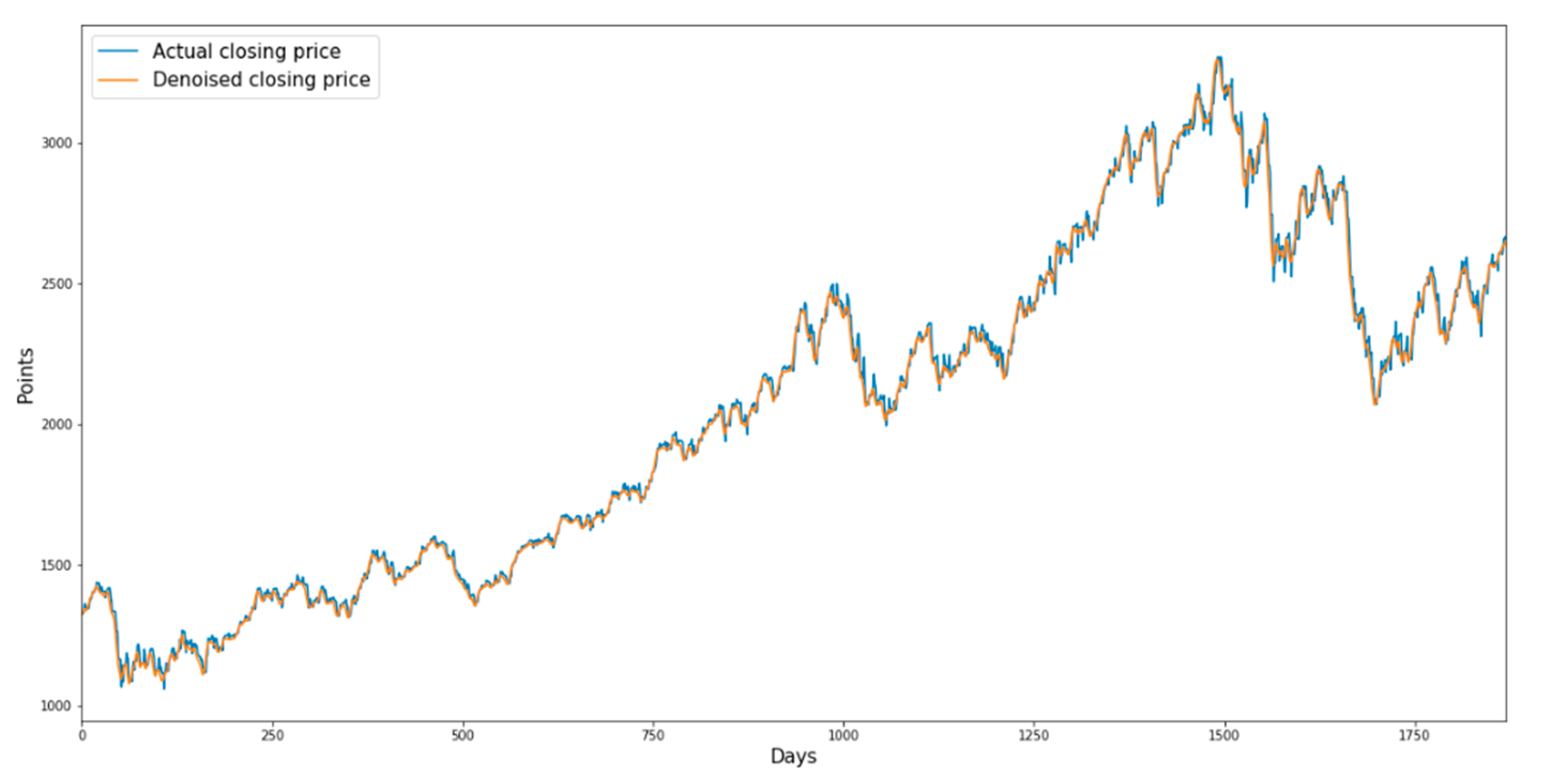
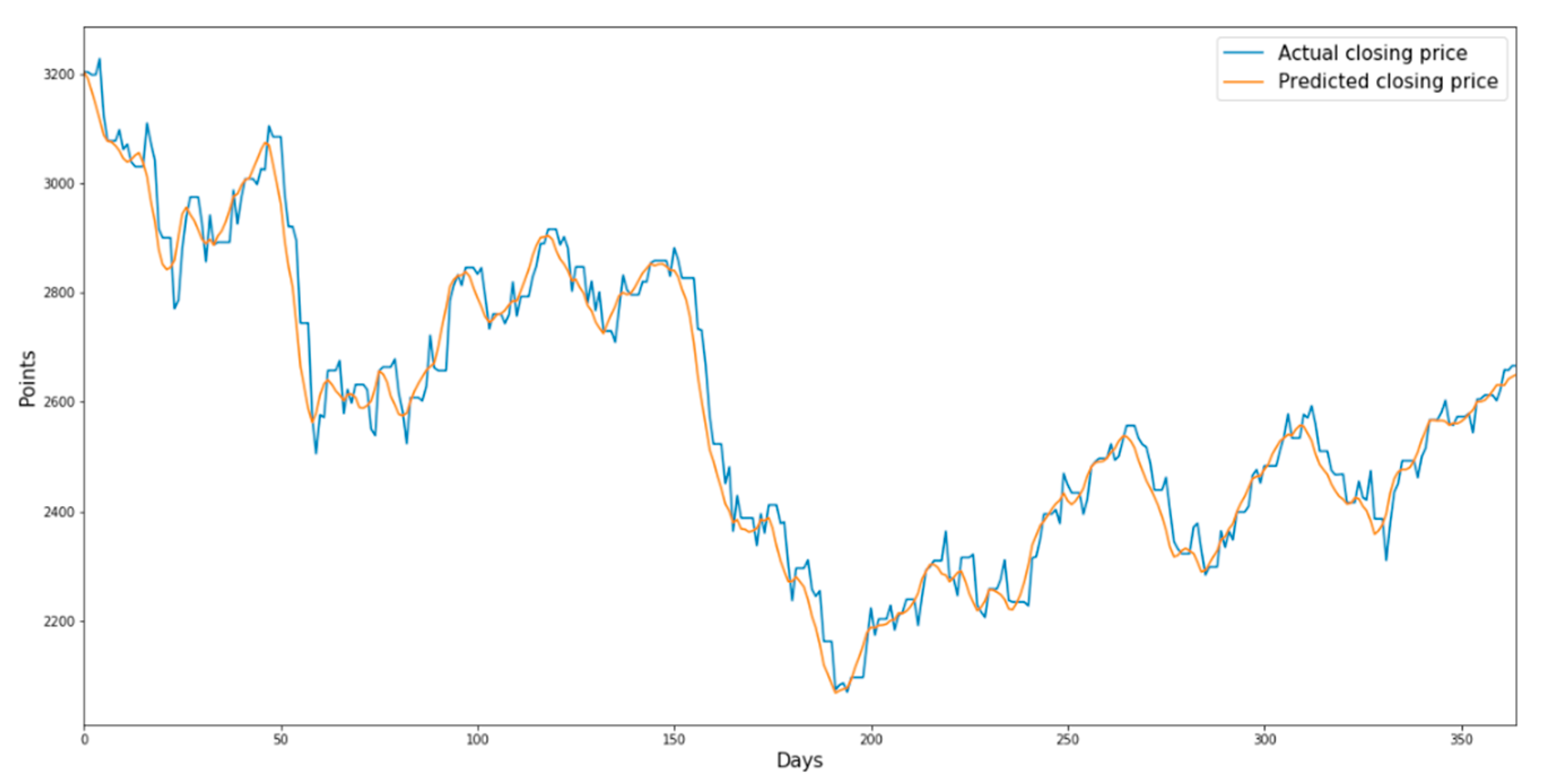
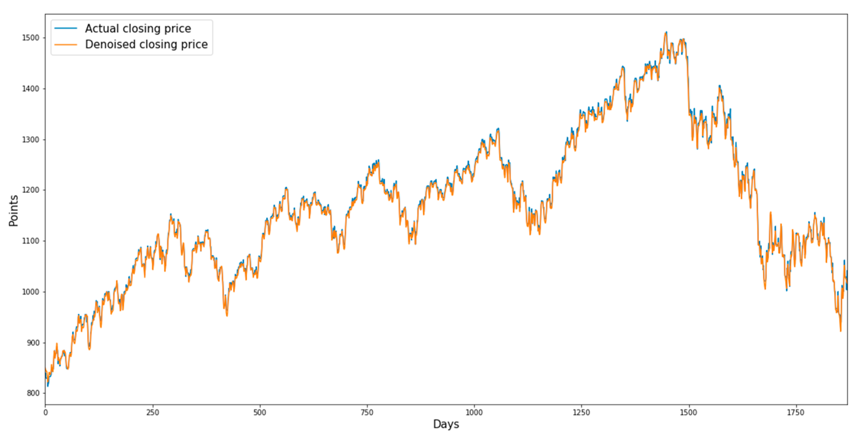
Figure 3,
Figure 4,
Figure 5 and
Figure 6 show the denoised closing prices and actual closing prices of the sector indices.
Figure 3 shows the graphs for the consumer discretionary sector index from 17 June 2003 to 16 March 2007, and
Figure 4 shows the graphs for the consumer staples sector index from 18 July 2006 to 17 July 2010.
Figure 5 and
Figure 6 show the graphs for the IT sector index and health care sector index from 17 June 2011 to 16 June 2015, respectively.
The denoised data obtained through the DAE are divided into a training dataset with 4 years of data and a validation dataset with 1 year of data, and then the LSTM model is trained. In the LSTM model training, the sequence length, learning rate, number of learning iterations, loss function, and optimization function were the same values as those used in the DAE. Using the data up to time
as input data, the predicted value at time
was obtained.
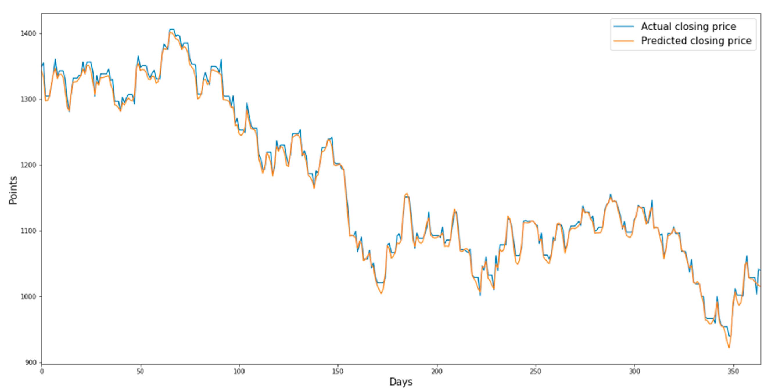
Figure 7 shows the predicted and actual prices of the consumer discretionary sector index from 17 June 2007 to 31 July 2008 when the validation dataset was used as the input data of the trained model. Similarly,
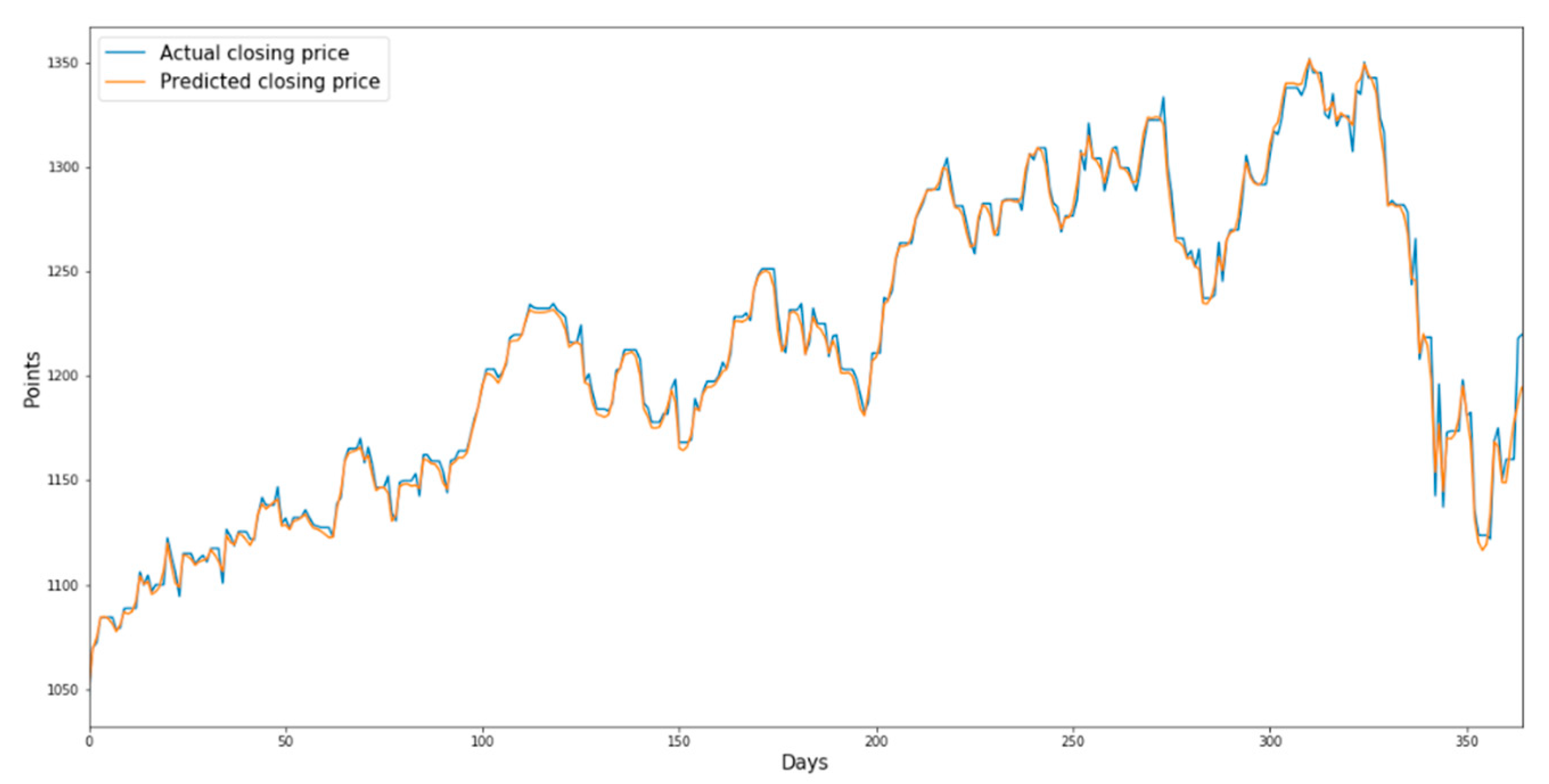
Figure 8 shows the predicted and actual prices of the consumer staples sector index from 18 July 2010 to 17 August 2011 when the validation dataset was used as the input data of the trained model. Finally,
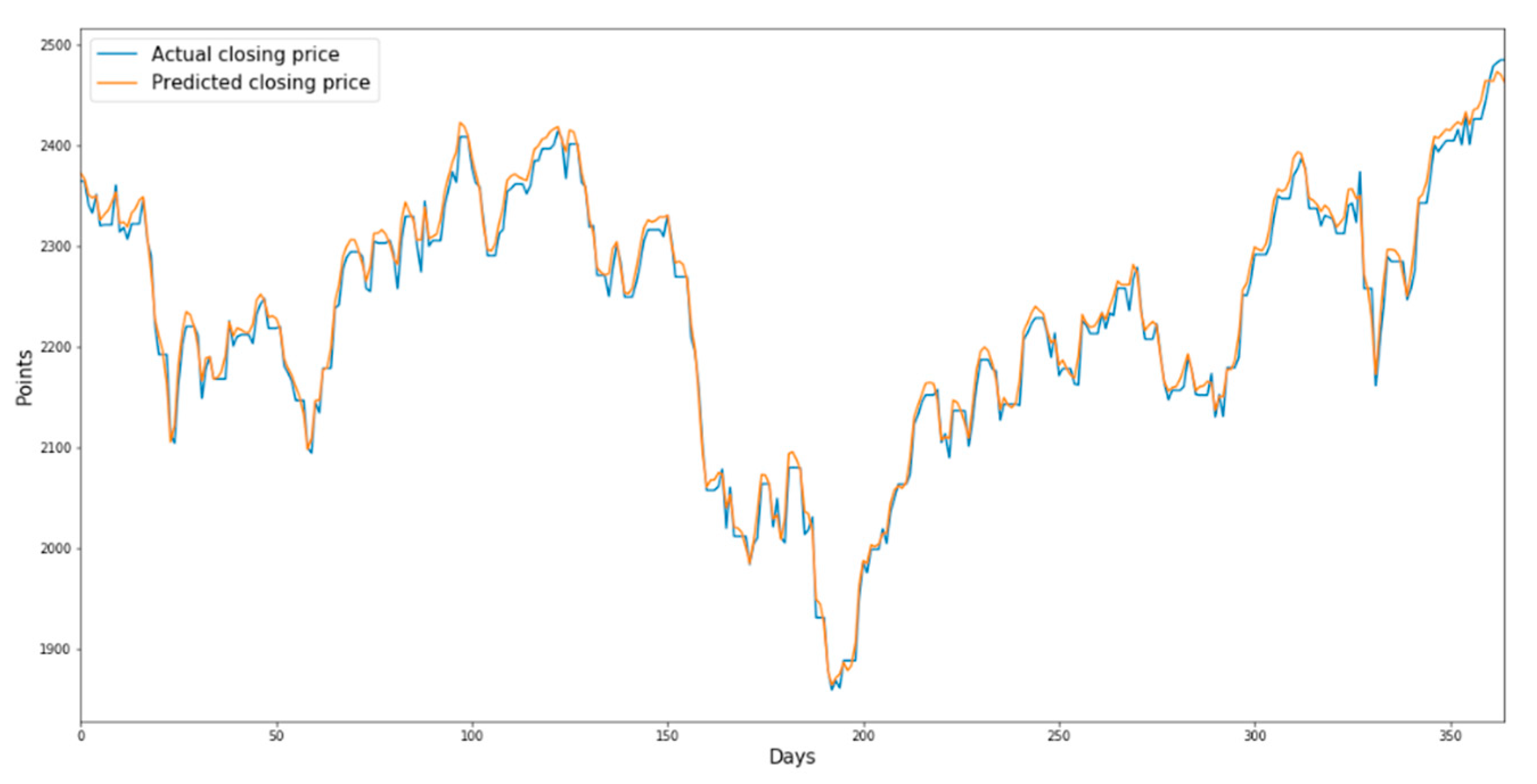
Figure 9 and
Figure 10 show the predicted and actual prices of the IT sector index and the health care sector index from 17 June 2015 to 31 July 2015 when the validation dataset is used as the input data of the trained model, respectively.
4.2. Repeat the Closing Price Prediction Using LSTM from
to
Repeating the same prediction as that performed in step 1, we obtain the predicted closing prices at
,
, …, and
. Given the denoised and predicted values from
to
, we calculated the mean squared error (MSE) for each sector to evaluate the DAE-LSTM model. The MSE is a loss function calculated as the square of the error, which is the difference between the predicted value and the actual value. The MSE is calculated as follows:
In Equation (4),
is the number of values,
is an actual value, and
is a predicted value.
4.3. Prediction of the Change Points Using Pettitt’s Test
Change point detection was performed using Pettitt’s test, as described in step 3, to check whether a significant change point existed in the predicted and actual data, and the date of a change point was recorded.
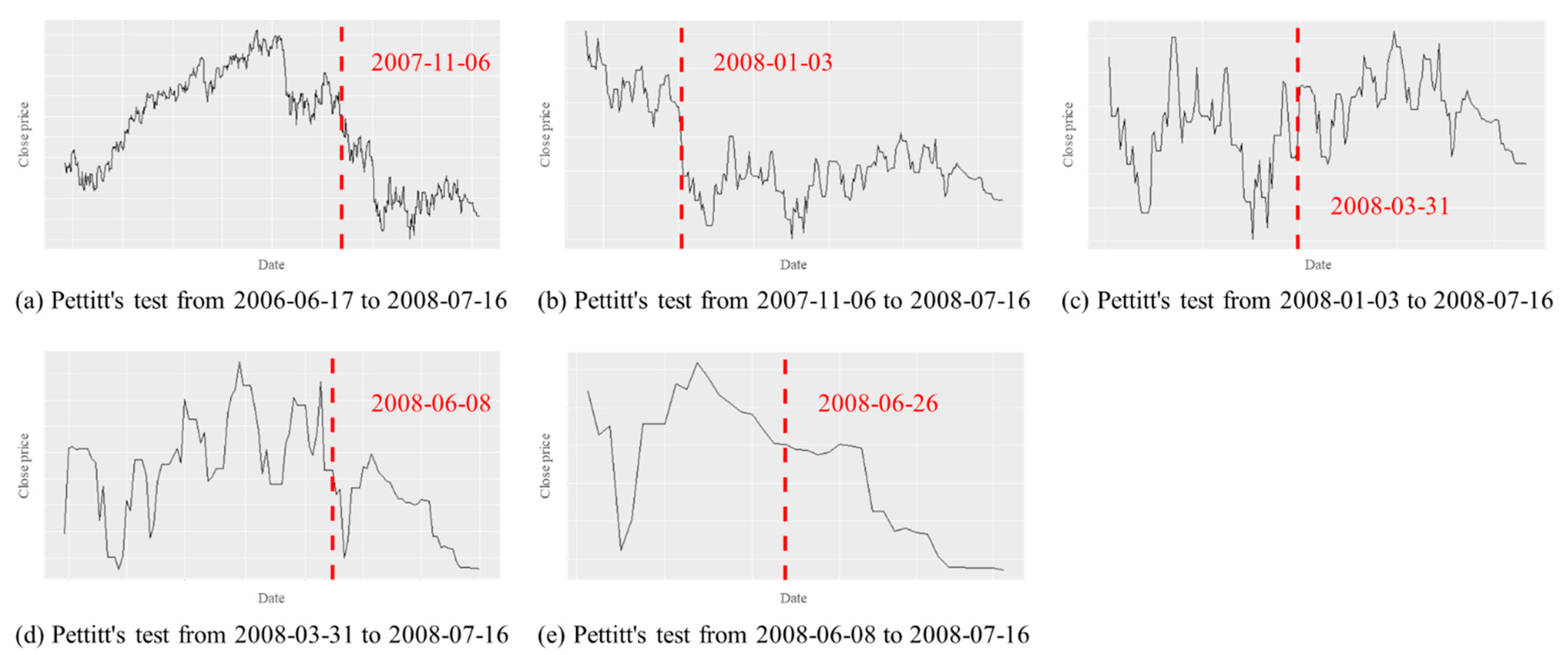
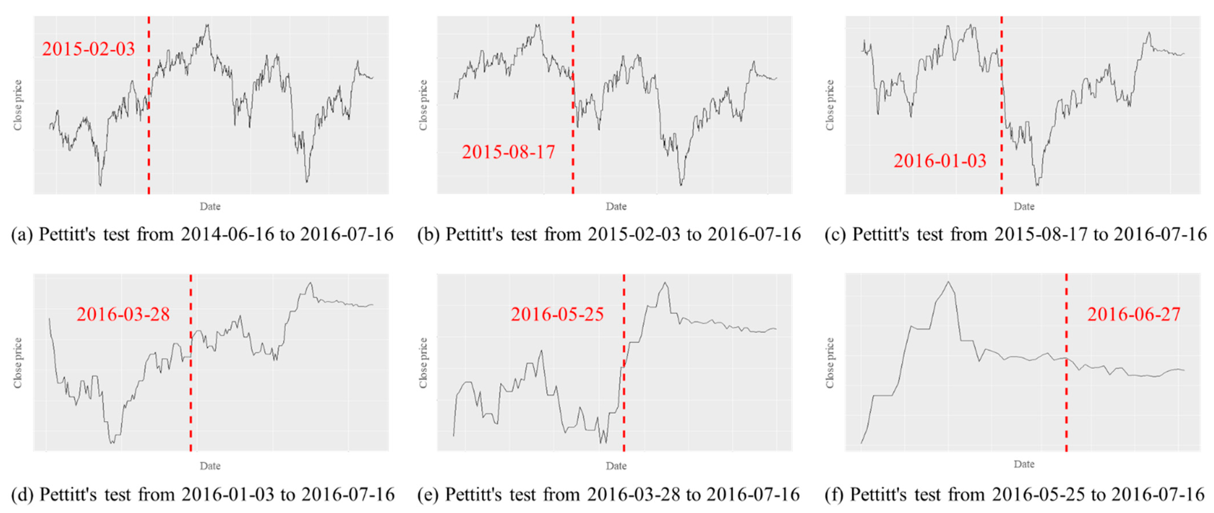
As shown in
Figure 15, in the case of the consumer discretionary sector index, Pettitt’s test was conducted on data from 17 June 2006 to 16 July 2008. During this time period, 6 November 2007 was detected as a change point, as shown in
Figure 15a. Then, as shown in
Figure 15b, Pettitt’s test was performed on the data from 6 November 2007 to 16 July 2008. In this case, 3 January 2008 was detected as a change point. By repeating this process, the first date of the change point detected later than the set time
in
Table 2 was selected as the final predicted change point date. In the case of the consumer discretionary index, since the set time
was 16 June 2008, 26 June 2008 was selected as the final predicted change point date, as shown in
Figure 15e.
In the same way as for the consumer discretionary sector index, Pettitt’s test is conducted for the consumer staples sector index (
Figure 16), IT sector index (
Figure 17), and health care sector index (
Figure 18) to select each final predicted change points.
Table 3 reports the dates when the change points occurred in the predicted and actual time series data by sector. It is interesting to note that the date of the predicted change point is found within 7 days prior to the start date of the trending upward phase for all sectors.
5. Discussion and Concluding Remarks
The purpose of this study was to use deep learning models to predict the change points that will appear in the future using the Russell 2000 industry index. Pettitt’s test, a statistical model, has been used to find the change points that only occurred in the past using historical data. Furthermore, this study contributes to predicting change points through a combination of statistical and deep learning models.
As shown in the empirical results, we were able to find a change point close to the actual start date of the uptrend for all sectors. Accurate prediction of change points in stock prices provides useful information, and the methodology that combines a deep learning model (DAE-LSTM) and a statistical model (Pettitt’s test) developed in this study can be utilized as a portfolio allocation strategy for investors in stock markets.
There are various assets traded in financial markets, and an enormous number of models or techniques for achieving efficient portfolios have been developed in the literature. Financial assets, investment techniques and investors are critical components in the efficiency of financial markets, and efficient financial markets have been well known to play an important role in sustaining economic growth. Investors in stock markets are able to achieve more efficient portfolios using our deep learning models. In this sense, our approach developed in this paper appears to contribute to the efficiency of financial markets, and hence, plays a role in sustaining economic growth.
It is expected that the methodology developed in this study can be applied not only to sector index data but also to individual stock data or various financial time series data, such as exchange rates, interest rates, and various macroeconomic indicators, to predict change points and use them for various purposes.
However, this study has potential limitations. The empirical results are limited to Russell 2000 stocks in four sectors. Based on our DAE-LSTM methodology, future research can enrich the topic by developing a new model that can be utilized for various types of financial time series data from global markets. In addition, the problem of LSTM prediction error could be improved by utilizing a deep learning model for better prediction of performance in future studies.
Author Contributions
Project administrator, K.O.; proposed the methodology, S.Y.; data curation and validation, S.J. (Sangyong Jeon); writing—original draft preparation, S.J. (Seunghwan Jeong) and H.R.; programming and formal analysis, T.P. and Y.C.; and writing—review & editing, H.L. All authors have read and agreed to the published version of the manuscript.
Funding
This work was supported by the National Research Foundation of Korea (NRF) grant funded by the Korean government (MSIT) (No. 2021R1A2C1094211).
Institutional Review Board Statement
Not applicable.
Informed Consent Statement
Not applicable.
Data Availability Statement
Not applicable.
Conflicts of Interest
The authors declare no conflict of interest.
References
- Hassan, M.R.; Nath, B.; Kirley, M. A fusion model of HMM, ANN and GA for stock market forecasting. Expert Syst. Appl. 2007, 33, 171–180. [Google Scholar] [CrossRef]
- Hassan, M.R. A combination of hidden Markov model and fuzzy model for stock market forecasting. Neurocomputing 2009, 72, 3439–3446. [Google Scholar] [CrossRef]
- Huang, S.C.; Wu, T.K. Integrating GA-based time-scale feature extractions with SVMs for stock index forecasting. Expert Syst. Appl. 2008, 35, 2080–2088. [Google Scholar] [CrossRef]
- Lachiheb, O.; Gouider, M.S. A hierarchical deep neural network design for stock returns prediction. Procedia Comput. Sci. 2018, 126, 264–272. [Google Scholar] [CrossRef]
- Rout, A.K.; Dash, P.K.; Dash, R.; Bisoi, R. Forecasting financial time series using a low complexity recurrent neural network and evolutionary learning approach. J. King Saud Univ. Comput. Inf. Sci. 2017, 29, 536–552. [Google Scholar] [CrossRef] [Green Version]
- Yan, B.; Aasma, M. A novel deep learning framework: Prediction and analysis of financial time series using CEEMD and LSTM. Expert Syst. Appl. 2020, 159, 113609. [Google Scholar]
- Cao, J.; Li, Z.; Li, J. Financial time series forecasting model based on CEEMDAN and LSTM. Phys. A Stat. Mech. Its Appl. 2019, 519, 127–139. [Google Scholar] [CrossRef]
- Jeon, S.Y.; Ryou, H.S.; Kim, Y.; Oh, K.J. Using Change-Point Detection to Identify Structural Changes in Stock Market: Application to Russell 2000. Quant. Bio-Sci. 2020, 39, 61–69. [Google Scholar]
- Vincent, P.; Larochelle, H.; Bengio, Y.; Manzagol, P.A. Extracting and composing robust features with denoising autoencoders. In Proceedings of the 25th International Conference on Machine Learning, Helsinki, Finland, 5–9 July 2008; pp. 1096–1103. [Google Scholar]
- Yang, J.H.; Kim, Y.; Oh, K.J. Forecasting the KOSPI 200 Stock Index Based on LSTM Autoencoder. Quant. Bio-Sci. 2020, 39, 101–109. [Google Scholar]
- Hochreiter, S.; Schmidhuber, J. Long short-term memory. Neural Comput. 1997, 9, 1735–1780. [Google Scholar] [CrossRef] [PubMed]
- Mallakpour, I.; Villarini, G. A simulation study to examine the sensitivity of the Pettitt test to detect abrupt changes in mean. Hydrol. Sci. J. 2016, 61, 245–254. [Google Scholar] [CrossRef] [Green Version]
- Conte, L.C.; Bayer, D.M.; Bayer, F.M. Bootstrap Pettitt test for detecting change points in hydroclimatological data: Case study of Itaipu Hydroelectric Plant, Brazil. Hydrol. Sci. J. 2019, 64, 1312–1326. [Google Scholar] [CrossRef]
- Csörgö, M.; Csörgö, M.; Horváth, L. Limit Theorems in Change-Point Analysis; Wiley Series in Probability and Statistics; Wiley: New York, NY, USA, 1997. [Google Scholar]
- Pettitt, A.N. A non-parametric approach to the change-point problem. J. R. Stat. Soc. Ser. C Appl. Stat. 1979, 28, 126–135. [Google Scholar] [CrossRef]
- FTSE Russell. Russell U.S. Equity Indexes. Available online: https://www.ftserussell.com/products/indices/russell-us (accessed on 8 August 2021).
- Petajisto, A. The index premium and its hidden cost for index funds. J. Empir. Financ. 2011, 18, 271–288. [Google Scholar] [CrossRef]
- Liu, P.; Zheng, P.; Chen, Z. Deep learning with stacked denoising auto-encoder for short-term electric load forecasting. Energies 2019, 12, 2445. [Google Scholar] [CrossRef] [Green Version]
- Romeu, P.; Zamora-Martínez, F.; Botella-Rocamora, P.; Pardo, J. Stacked denoising auto-encoders for short-term time series forecasting. In Artificial Neural Networks; Springer: Cham, Switzerland, 2015; pp. 463–486. [Google Scholar]
- Zhao, Y.; Ren, X.; Zhang, X. Optimization of a Comprehensive Sequence Forecasting Framework Based on DAE-LSTM Algorithm. J. Phys. Conf. Ser. 2021, 1746, 012087. [Google Scholar] [CrossRef]
- Oh, K.J.; Han, I. Using change-point detection to support artificial neural networks for interest rates forecasting. Expert Syst. Appl. 2000, 19, 105–115. [Google Scholar] [CrossRef]
- Oh, K.J.; Kim, K.J. Analyzing stock market tick data using piecewise nonlinear model. Expert Syst. Appl. 2002, 22, 249–255. [Google Scholar] [CrossRef]
Figure 1.
Structural diagram of a denoising autoencoder (DAE).
Figure 1.
Structural diagram of a denoising autoencoder (DAE).
Figure 2.
Proposed model.
Figure 2.
Proposed model.
Figure 3.
Denoised closing prices and actual closing prices of the consumer discretionary sector index.
Figure 3.
Denoised closing prices and actual closing prices of the consumer discretionary sector index.
Figure 4.
Denoised closing prices and actual closing prices of the consumer staples sector index.
Figure 4.
Denoised closing prices and actual closing prices of the consumer staples sector index.
Figure 5.
Denoised closing prices and actual closing prices of the IT sector index.
Figure 5.
Denoised closing prices and actual closing prices of the IT sector index.
Figure 6.
Denoised closing prices and actual closing prices of the health care sector index.
Figure 6.
Denoised closing prices and actual closing prices of the health care sector index.
Figure 7.
Prediction chart of the consumer discretionary sector index using LSTM for the validation dataset.
Figure 7.
Prediction chart of the consumer discretionary sector index using LSTM for the validation dataset.
Figure 8.
Prediction chart of the consumer staples sector index using LSTM for the validation dataset.
Figure 8.
Prediction chart of the consumer staples sector index using LSTM for the validation dataset.
Figure 9.
Prediction chart of the IT sector index using LSTM for the validation dataset.
Figure 9.
Prediction chart of the IT sector index using LSTM for the validation dataset.
Figure 10.
Prediction chart of the health care sector index using LSTM for the validation dataset.
Figure 10.
Prediction chart of the health care sector index using LSTM for the validation dataset.
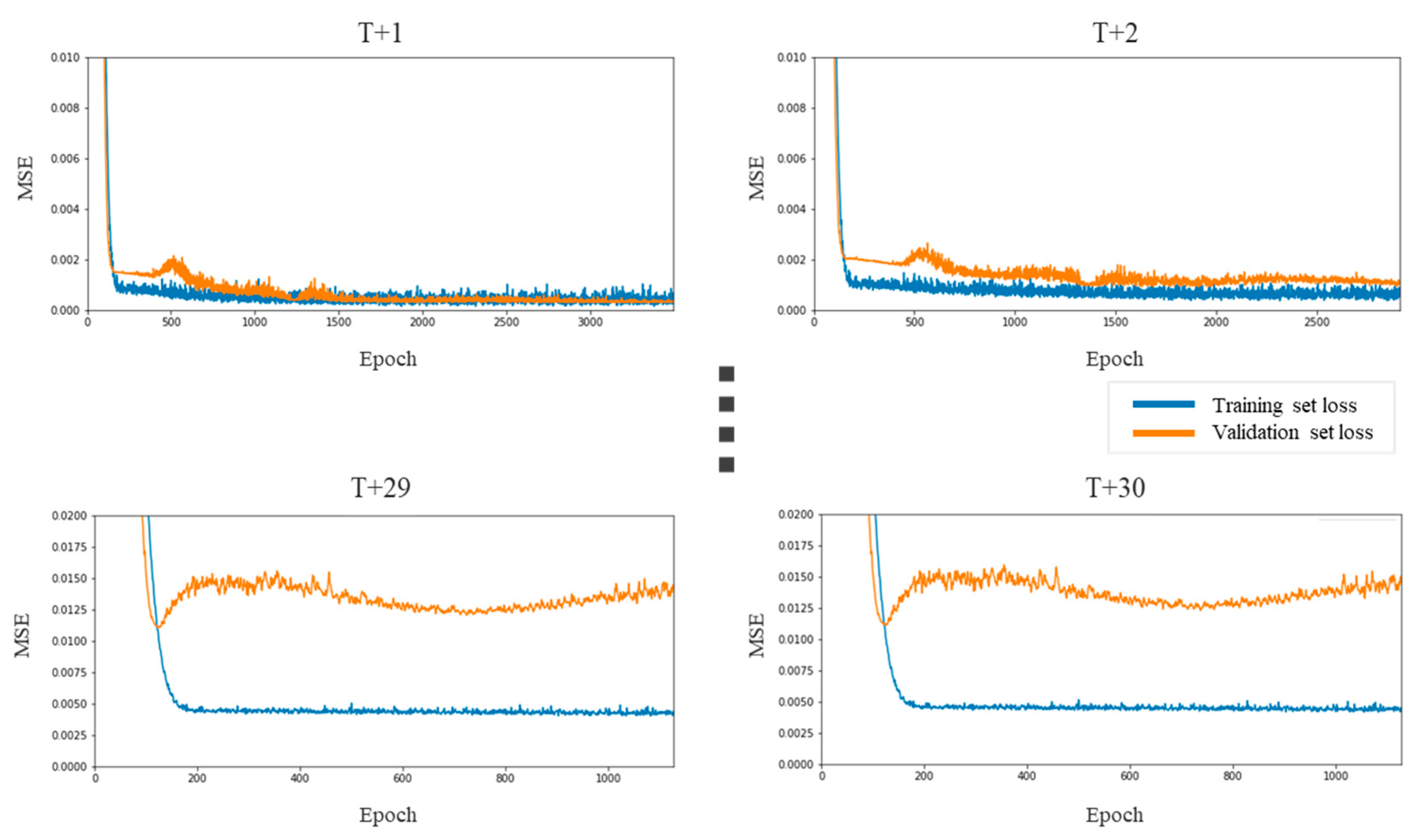
Figure 11.
LSTM prediction errors for the consumer discretionary sector.
Figure 11.
LSTM prediction errors for the consumer discretionary sector.
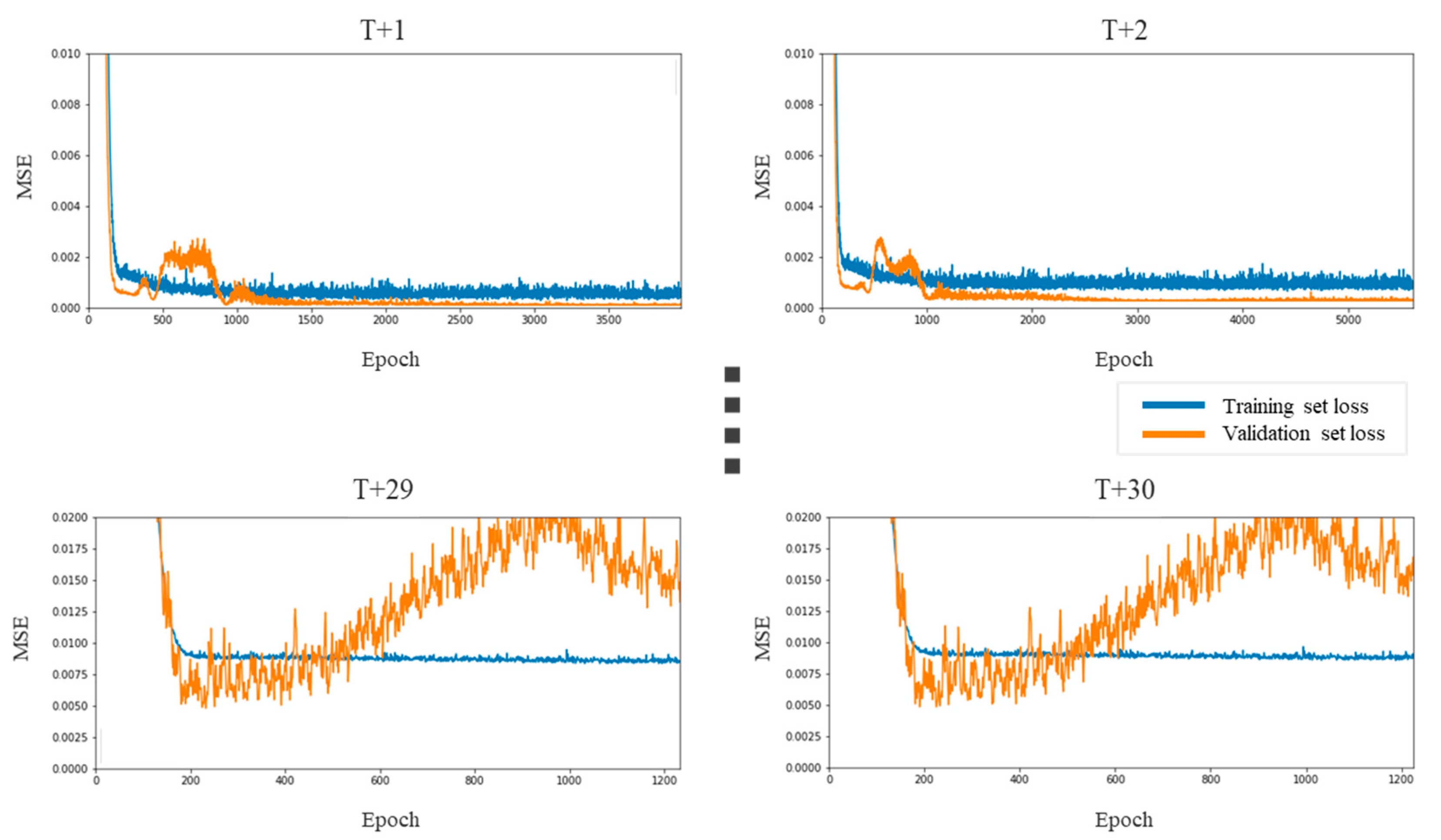
Figure 12.
LSTM prediction errors for the consumer staples sector.
Figure 12.
LSTM prediction errors for the consumer staples sector.
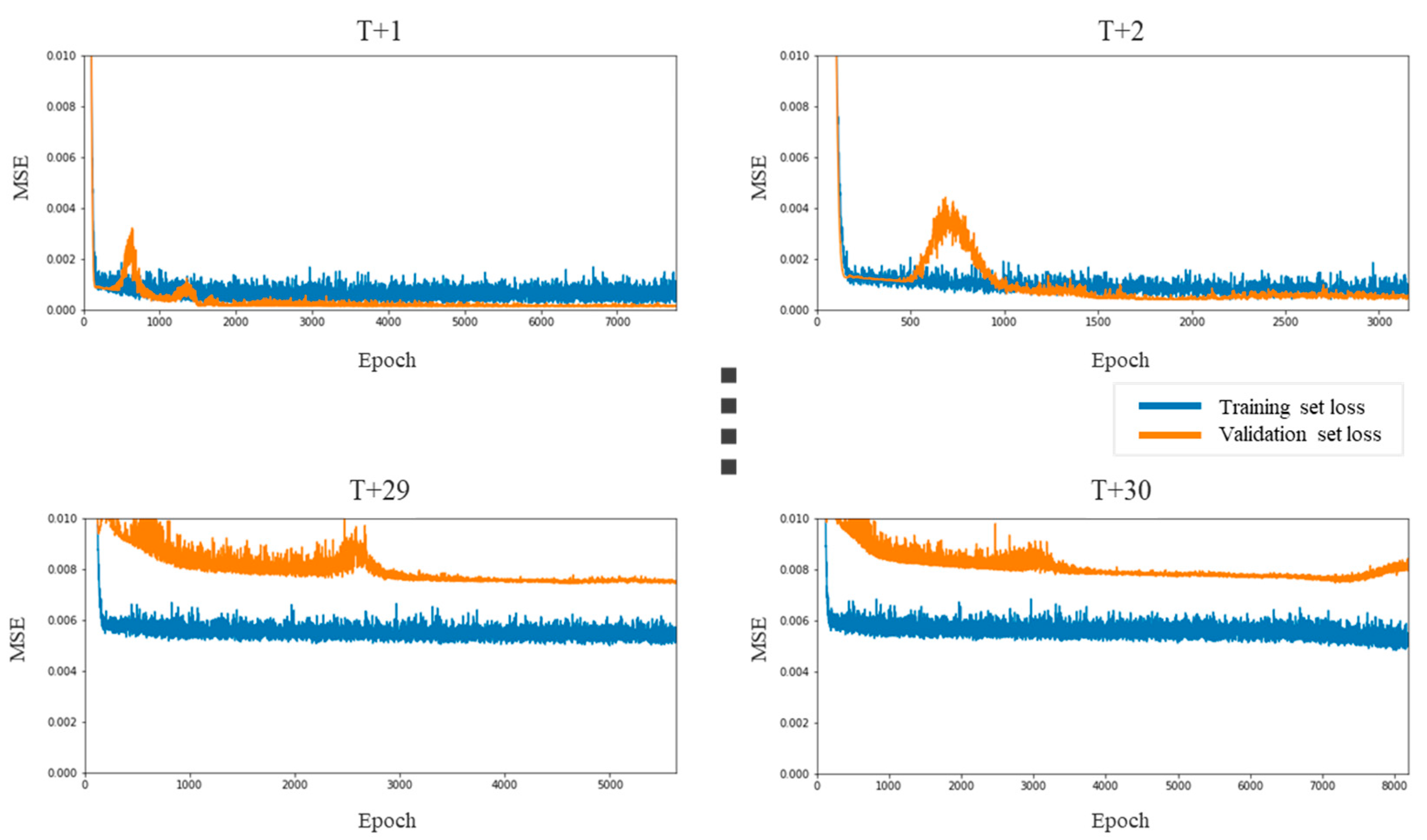
Figure 13.
LSTM prediction errors for the IT sector.
Figure 13.
LSTM prediction errors for the IT sector.
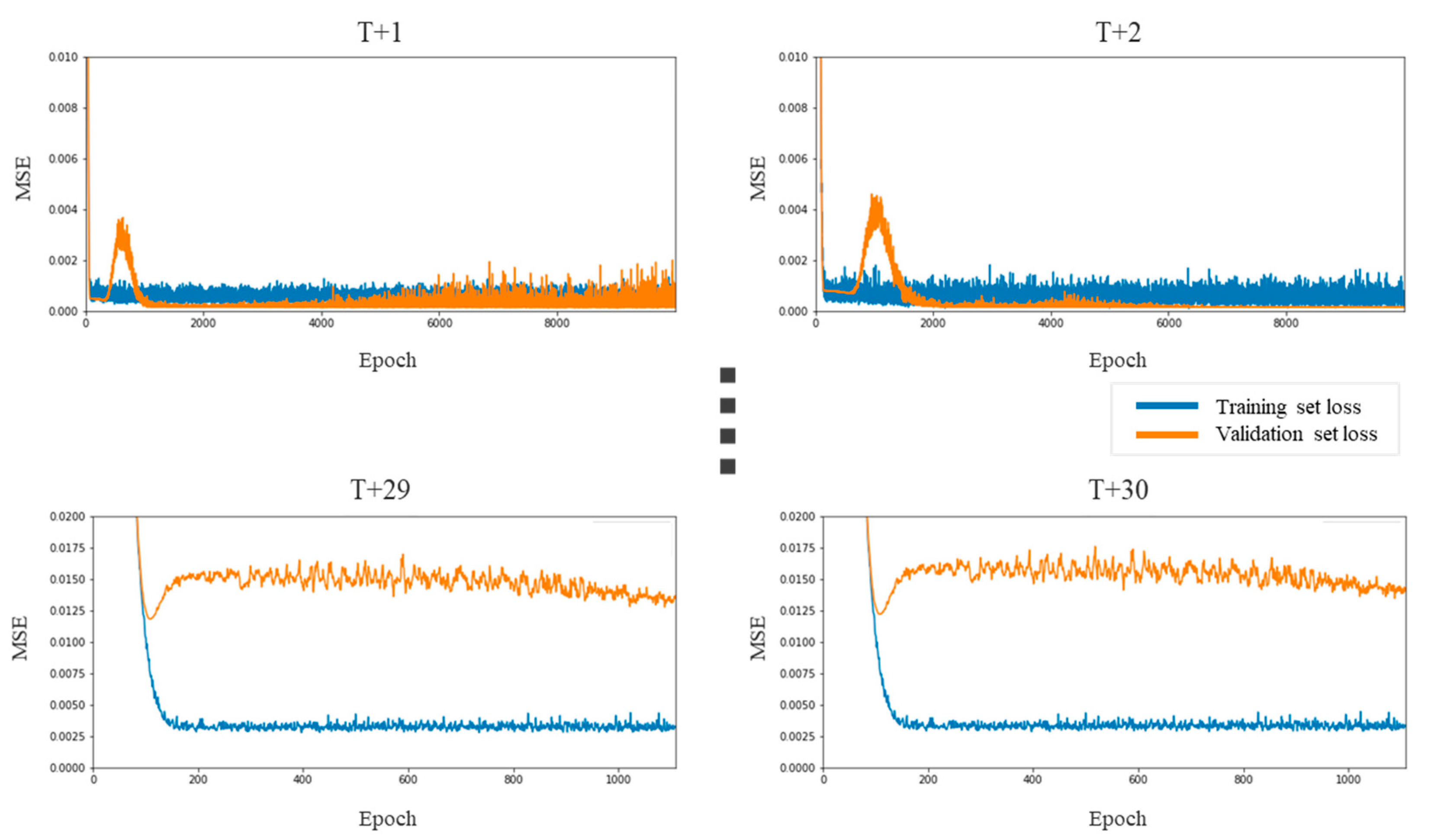
Figure 14.
LSTM prediction errors for the health care sector.
Figure 14.
LSTM prediction errors for the health care sector.
Figure 15.
Pettitt’s test for the consumer discretionary sector index.
Figure 15.
Pettitt’s test for the consumer discretionary sector index.
Figure 16.
Pettitt’s test for the consumer staples sector index.
Figure 16.
Pettitt’s test for the consumer staples sector index.
Figure 17.
Pettitt’s test for the IT sector index.
Figure 17.
Pettitt’s test for the IT sector index.
Figure 18.
Pettitt’s test for the health care sector index.
Figure 18.
Pettitt’s test for the health care sector index.
Table 1.
Start date of the uptrend of Russell 2000 stocks by sector.
Table 1.
Start date of the uptrend of Russell 2000 stocks by sector.
| Sector | Uptrend Start Date (yyyy–mm–dd) |
|---|
| Consumer Discret. | 2008–07–01 |
| Consumer Staples | 2011–08–01 |
| IT | 2016–07–01 |
| Health Care | 2016–07–01 |
Table 2.
Time t by sector.
Table 2.
Time t by sector.
| Sector | Interval of Change Points | t (yyyy–mm–dd) | Start Date of Uptrend (yyyy–mm–dd) |
|---|
| Consumer Discret | 24.68 | 2008–06–16 | 2008–07–01 |
| Consumer Staples | 23.71 | 2011–07–17 | 2011–08–01 |
| IT | 29.47 | 2016–06–16 | 2016–07–01 |
| Health Care | 23.42 | 2016–06–16 | 2016–07–01 |
Table 3.
Predicted and actual change points by sector.
Table 3.
Predicted and actual change points by sector.
| Sector | Predicted Change Point Date (yyyy–mm–dd) | Actual Change Point Date (yyyy–mm–dd) |
|---|
| Consumer Discret | 2008–06–26 | 2008–07–01 |
| Consumer Staples | 2011–07–25 | 2011–08–01 |
| IT | 2016–06–27 | 2016–07–01 |
| Health Care | 2016–06–24 | 2016–07–01 |
| Publisher’s Note: MDPI stays neutral with regard to jurisdictional claims in published maps and institutional affiliations. |
© 2021 by the authors. Licensee MDPI, Basel, Switzerland. This article is an open access article distributed under the terms and conditions of the Creative Commons Attribution (CC BY) license (https://creativecommons.org/licenses/by/4.0/).


 ,
, 


