Optimal Internet of Things Technology Adoption Decisions and Pricing Strategies for High-Traceability Logistics Services

Abstract

The Internet of Things (IoT) technology-based tracking system can reduce freight loss/damage during delivery, thereby avoiding wasting social resources. In this study, we address the issue of whether an E-retailer with a logistics arm should provide high-traceability logistics value-added service (based on IoT technology) in two customer segments and analyze their pricing decision. We found that companies always adopt IoT when equipment operation cost is low and not when the cost is high. Otherwise, the optimal IoT adoption strategy for a company depends on multiple factors, for example, the internal operation efficiency of a company. Providing high-traceability service as one kind of public service does not necessarily optimize social welfare even if the overall delivery failure is reduced. The customers’ preference for traceability significantly affects the company’s decision. Hence, we suggest that the company should implement a comprehensive investigation before launching a specific strategy.

1. Introduction

In 2020, the average daily express processing volume of Chinese express enterprises exceeded 230 million, and the annual express business volume exceeded 83.36 billion [1]. The global E-commerce sector shows a dramatic increase in its share of all retail sales from 16% in 2019 to 19% since the COVID-19 pandemic [2].

As E-commerce is blooming, the influence of a fast-growing express industry on the environment is getting significant. In the top 100 cities globally, the carbon emission volume caused by the shipping industry is 19 million tons, and emissions from delivery traffic will increase by 32% in 2030 [3]. In addition, in E-commerce shipping, the use of plastic packaging and air pillows further strengthens the effect on the environment [4]. When delivery failure happens, for example, lost or damaged freight (caused by theft, rough handling, and misoperation) during the transportation, the whole logistics activity becomes an ineffective operation, which only wastes social resources and deepens environmental pollution. The delivery failures are on the rise, where 56% of the US customers have received damaged parcels in 2018 [5] and the loss and damage of parcels accounted for 17.7% and 11.7% of the total valid complaints of consumers in the Chinese express industry, respectively [6]. Of the examples listed above, the common feature is that tracking back to the source (responsible party) of delivery failure is difficult. The inability to trace the logistics process in a real-time manner is common in the present industry.

The freight damage rate and logistics information transparency (location of the goods, the route of goods transportation, and the distance from destination) have an important effect on customers’ satisfaction [7]. The National Association of Citizens Advice Bureau of The United Kingdom [8] claimed that the delivered problems, such as loss or damaged parcel, cause UK consumers a GBP 85 million loss. For an individual customer, fixing a parcel issue takes an average of 2 h and GBP 15.50, and some customers even become stressed and anxious. Customer dissatisfaction will affect E-retailer’s long-term competitiveness.

However, the recent technology development, such as the Internet of Things (IoT)-based high logistics traceability solution, is promising to help firms overcome the challenges that arise from the lack of comprehensive real-time logistics information, ensuring product quality and integrity [9]. The commonly used IoT equipment includes radio-frequency identification devices (RFID), Global Positioning System (GPS), and other sensors [9]. In the shipping industry, RFID offers protection against theft and fraud and helps businesses track damage, loss, error, expiration, and increases overall accuracy [10]. Except for fraud, theft, and process errors, the RFID system can also detect freight damage, combined with additional sensors, such as shock and impact recorders, vibration sensors, and temperature monitors. The system can reveal any drops, shocks, or impacts that could damage shipment, and thus, the responsible party can be easily confirmed [11].

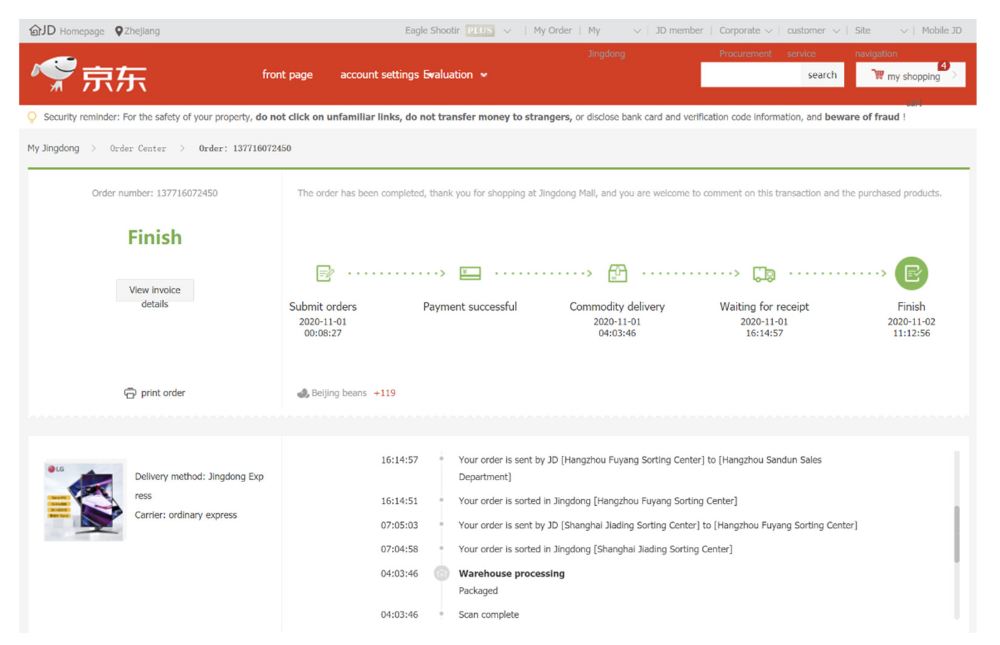
Nowadays, customers can acquire real-time location information of their same-day delivery orders [12]. However, such service is not popular in conventional e-commerce logistics services, and most logistics service providers (LSPs) only provide customers with fragmented information. Figure 1 shows that JD, as an E-retailer with its own logistics arm, only provides the information of packages entering and leaving a certain warehouse if customers choose basic logistics service. The responsible party could not be easily recognized when the cargos are damaged or lost. However, by introducing the high-traceability system, the firm can acquire real-time logistics information. For example, IoT innovator Hanhaa provides the IoT hardware “ParceLive”, which can provide highly accurate GPS tracking, record temperature/humidity, and identify if the freight has been dropped or opened. This postcard-sized equipment can easily be inserted into a parcel. The real-time logistics information can be accessed on ParceLive Portal [13].Two LSPs, Sigma Retail Solutions, and Avarto Bertelsmann adopt the ParceLive in their services and intend to satisfy customers’ need for real-time logistics information, enhance customers’ confidence in service quality, and reduce the burden of customer support [14]. Except for ParceLive, many other IoT-based logistics high-traceability solutions (also refers to the tracking system) are promoted. Roambee [15] provides the industry’s first end-to-end wireless Bluetooth Low Energy (BLE) tags/GPS/Wi-Fi-based monitoring solution. The company that adopts the solution of Roambee can customize the traceability level, at a vehicle, container, pallet, or shipment level. Arviem provides real-time, carrier-independent data on the cargo condition (location, estimated time of arrival, temperature and humidity, door opening and light intrusion, shock) during the whole journey. Customers can view all freight movements and other conditions in real-time on an interactive map. The service can minimize the risk of damage and theft [16]. Adopting IoT technology significantly promotes logistics operation efficiency. The leading less-than-truckload (LTL) company in the US, Old Dominion FreightLine, Inc., invests in improving logistics traceability and reducing the freight loss from 1.5% to 0.2%, which is 60% lower than the industry average level [17]. By continuously updating and optimizing information systems, YTO Express (Famous Chinese LSP) reduced the complaint rate by 92.89% in 2019 compared with that in 2018 [18].

In fact, E-retailers including Alibaba, TAOBAO, and JD also develop IoT-based tracking system [19,20]. JD’s logistics arm launched a value-added service (VAS) called “Feather Letter”, which can also provide their customers the accurate logistics information in a real-time manner [20].

Logistics performance significantly affect customers loyalty in e-commerce [21]. Therefore, for an E-retailer as JD, providing a high-traceability logistics service as a VAS will enhance the firm’s profitability while optimizing customers’ experience. VAS refers to the unique or specific activities that firms can jointly develop to enhance their efficiency, and eventually provide competitive advantages in the marketplace [22,23]. VAS determines the level of express enterprises, and by providing VAS, LSP can enter different market segments and open up new profit sources [24]. In total, 88% of customers want to acquire real-time logistics information throughout the whole delivery process [5]. UPS provides real-time freight tracking for expensive delivery services, such as UPS Air since 2016 [25]. Customers trust UPS for its comprehensive tracking system [26]. According to a report from the Boston Consulting Group, more than 85% of Chinese consumers who are born after 1990 frequently use Cainiao’s mobile software to check logistics information [27]. This result indicates customers’ preference for the availability of logistics information (Cainiao is a leading logistics company in China).

To summarize, for E-retailer with a logistics arm, the benefits of providing an IoT-based high-traceability logistics service as VAS are threefold:

• Reduce the probability of loss and damage of freight and avoid the social resource waste (including freight value loss, compensation cost to customers, and the companies’ internal communication cost for resolving delivery failure);
• Satisfy customers’ demand for high-traceability logistics services;
• Enhance the profitability by achieving the first two advantages.

Given the rapid development of the IoT-based high-traceability system, this research aims to understand the influence of traceability on logistics service operations. To be specific, we will investigate the following research questions in the study. First, how will the poor delivery quality affect the company’s profitability? What can the company do? Second, how does high-traceability service affect the company’s pricing decision? Third, what factors affect the company’s high-traceability service adoption decision?

We build stylized models about the optimal IoT adoption decisions of an E-retailer with a self-built logistics arm serving two customer segments, namely, traceability sensitive (TS) and traceability not sensitive (TNS) customers. The customer differs in their sensitivity on logistics traceability. TS customers enjoy the benefits of high-traceability logistics service. For example, they can arrange their schedule freely rather than wait at home if an accurate estimated time of arrival is provided. Thus, TS customers are willing to pay more for the VAS, while such benefits might be less attractive to TNS customers. The E-retailer provides free shipping (basic logistics service) for customers who buy their product and provide high-traceability service as a VAS, which is consistent with the current practice of JD. We examine the performance of several different IoT adoption strategies, which differ in the logistics service traceability level launched in both segments. When basic logistics service is provided, the probability of delivery failure occurring is high, and a corresponding cost could be incurred. When high traceability is introduced, the delivery quality is improved while the IoT operation cost is incurred. To clarify, as Dickey [14] illustrated the definition of “Track & Trace”, “Real-time Tracking”, and “Monitoring”, the high logistics traceability in our research is the same as the concept of Monitoring. The company can monitor several indicators of in-transit freight in real-time, and the indicators include location, temperature, and shock, etc.

Our findings are summarized as follows. First, we found that providing a high compensation rate can effectively enhance profitability, but the premise is that the delivery quality is solid. Second, we characterize the company’s optimal pricing decision and profit under each strategy. We also derive the company’s optimal IoT adoption strategy transfer paths which are characterized by the company’s communication cost and IoT operation cost. The company always chooses to adopt IoT when equipment operation cost is low and not when the cost is high. However, when the IoT cost is at the intermediate level, two strategies could be optimal. One is the differentiated strategy that serves the TNS segment with basic service and serves TS with high-traceability service. The other one is the High-End strategy that excludes the TNS segment and serves TS with high traceability. Third, we consider the situation where the company can acquire full information by analyzing consumer big data. The full information advantage extends the feasible range for the differentiated strategy to be optimal.

Our contributions are as follows. We characterize E-retailer’s problem about whether to provide high-traceability service as VAS. We prove that the E-retailer has sufficient incentive to improve delivery quality. We clarify in what condition the company shall choose to adopt the IoT tracking system in their business model and the pricing of the services. However, the effective implementation of promoted findings depends on the company’s understanding of their customers, selection of IoT solution suppliers, and company operational efficiency. Therefore, the company is suggested to make use of big data with data mining, machine learning, or deep learning techniques to extract the customers’ willingness to pay (WTP) for logistics traceability. Moreover, the company should implement a comprehensive market investigation to select appropriate IoT solutions. Optimizing the company structure to reduce internal communication costs could also be appropriate for small E-retailer if they cannot acquire the IoT system at a low cost.

The remainder of this paper is structured as follows. After the review related literature stream in Section 2, the model will be introduced in Section 3. We launch a comprehensive analysis of LSP’s pricing decision and IoT adoption decision in Section 4. The conclusion is given in Section 5. All proofs are presented in the Appendix A.

2. Literature Review

2.1. Logistics Service Pricing

Our work is related to the logistics service pricing literature. Some scholars promoted the pricing strategy based on distance and freight volume [28,29] or freshness of perishable freight [30,31]. By contrast, our pricing strategy is related to the delivery failure rate, which is caused by the misoperation of the logistics team. Wang and Li [32] investigated a supply chain including a manufacturer, an e-commerce platform, and an LSP. The logistics fee is paid by the manufacturer or platform which depends on who has the dominant position, and either way, the logistics fee will finally be covered by the product price with free shipping (PPFS) paid by the consumer. In our context, the free-shipping policy is adopted; however, the E-retailer has its own logistics arm for delivery rather than outsource to LSP. Lukassen and Wallenburg [33] conducted qualitative research on the origin and categorization of logistics pricing and discussed the relationship between logistics pricing and industrial service pricing. Our work is also related to research on the pricing of value-added logistics services as the corresponding literature is scant. Liu, W. et al. [34] built an analytical model for an Online to Offline service platform’s pricing decision of VAS. In their research, the suppliers on the platform provide basic service, and the platform’s investment in VAS directly enhances customer’s demand but does not affect the service quality. However, in our work, basic service and VAS are fulfilled by the company, and VAS will affect service quality and customer utility.

2.2. Traceability in Supply Chain Management

Our work is related to research about traceability in supply chain management. The food and medicine industries are two of the few industries that widely adopt traceability systems [35]. Ensuring a safe supply is a difficult in food supply chains task where information asymmetry exists [36], and recalling specific batches of products are common in the food/medicine industries, however, adopting the traceability system significantly reduces social risk. Aung and Chang [37] summarized the advantages of the traceability system including reducing the food recall cost after an accident by compressing the recall scale. The system can promptly warn the company to reduce the possibility of a recall event. However, traceability in the above industries does not necessarily improve product quality. Resende-Filho and Hurley [38] indicated that traceability is not a clear signal for safe food, and government regulations based on mandatory traceability and sanctions do not necessarily lead to food safety. Starbird and Amanor-Boadu [39] showed that too high or too low traceability will affect the profit distribution between producers and processors, which will lead to producers providing less reliable products. Sun and Wang [40] analyzed a procurement problem in the food industry, and their research was conducted in the scenario where traceability can/cannot improve product quality. Traceability is an additional attribute that is independent of tangible product quality; hence, traceability can relieve the consequence of food recall but not avoid it. By contrast, traceability in the logistics industry directly affects the service quality (delivery failure rate), making our study differ from the aforementioned works. Some scholars emphasize the integration of traceability information and supply chain operation can improve the firm’s operational performance [41,42]. Wang, X. et al. [41] shows the benefits of integrating traceability systems with supply chain management processes through case study analysis. Wang, X. et al. [42] build an integrated optimization model about optimal production planning which combines product safety related traceability factors with operations factors. Similarly, our work also addresses how traceability can be incorporated into a firm’s operation decision and improve the operation performance eventually.

2.3. IoT Technology Adoption in Supply Chain Management

Finally, our study is related to the literature about IoT technology adoption in supply chain management. de Vass et al. [43] conduct a survey-based study that reveals that multiple forms of IoT technology are adopted in Australian retail supply chains, and find a positive effect of IoT adoption on supply chain integration (with customers) and supply chain performance. de Vass et al. [44] analyze the interviews with managers from the Australian retail industry and prove IoT adoption can improve the company’s sustainability. Our work focuses on one specific application of IoT in e-commerce, where an E-retailer adopts IoT technology as a measure to offer customer real-time logistics traceability, we discuss whether both parties can benefit from such interaction. Rekik et al. [45] indicate that various errors in warehouse operations could lead to a discrepancy between real inventory level and record in the information system, which affects customers’ services level. Some studies [46,47] reveal the performance of launching IoT equipment on reducing the inventory shrinkage (inventory shrinkage means inventory discrepancy caused by loss, damage, or misplacement of inventory). Tao et al. [48] studied the multiperiod inventory control policy with and without RFID adoption. They found that the inventory policy with RFID adoption was much more stable than that without RFID. Fan et al. [49] investigated RFID adoption in the supply chain, which consists of one supplier/manufacturer and one retailer, and found that the RFID is advantageous regardless of the inventory inaccuracy level. Biswal et al. [50] introduced the RFID technology to solve the inventory shrinkage problem in the humanitarian supply chain. Qin et al. [51] studied how supply chain members could apply RFID technology to mitigate the bullwhip effect. The feature of IoT adoption reducing misplacement of freight is kept in our research, and we focus on how IoT adoption affects freight misplacement in multi-stage transportation rather than the freight shrinkage in the single warehouse. The adoption of IoT technology will be more meaningful as the freight is more likely to be misplaced when different logistics teams hand over the freight sequentially. Chadha et al. [52] provide IoT-based logistics policies, and indicate incorporating IoT technical into traditional logistics consolidation strategy will enhance the sustainability of the unimodal freight delivery system. For more detailed literature reviews on how IoT technology disrupts the supply chain management please refer to Ben-Daya et al. [53].

2.4. Contribution to Literature

Our work contributes to the literature on several fronts. First, we focus on the E-retailer’s practice of providing high-traceability logistics service as VAS, which is not yet discussed by the previous literature. Furthermore, consistent with the IoT technology adoption practice in supply chain management, our model equips the logistics team with IoT equipment to reduce misoperation probability and provide real-time logistics information in multi-stage delivery, which affects the company’s profitability and customer utility. All those factors allow our model to yield an ample analysis of E-retailer’s IoT adoption decisions. Finally, our results shed some light on how the free-shipping policy will affect the company’s decision on VAS.

3. Model

Our research is based on the following setting: an E-retailer who provides free shipping for the product sold on their website and uses self-built logistics service arm to deliver those freights (e.g., JD and Vipshop in China). The E-retailer is a monopoly, which is reasonable for the customers to only prefer to buy a certain type of product from this E-retailer. For example, Chinese customers prefer to purchase cosmetics on Vipshop and Consumer Electronic on JD. For brevity, we name this E-retailer as “the company” in the rest of the paper. The company’s profit is affected by delivery quality. If the freight is damaged or lost during delivery, then the E-retailer needs to compensate the customers, and other costs might incur. The company can reduce the probability of delivery failure (e.g., freight damage or loss) by adopting a high-traceability logistics system but not being able to eliminate the risk.

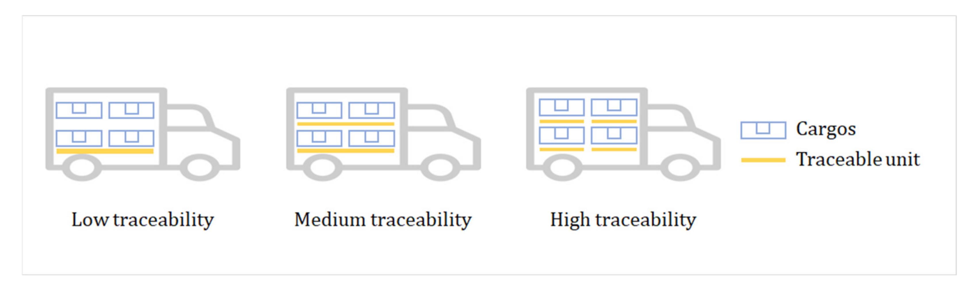
The freight passes several distribution centers until arriving at the designation, and in the meantime, several logistics teams will deliver the freight in a sequential manner (different teams responsible for different logistics legs). The parcel will be loaded into a smart pallet with IoT equipment during transportation. In our study, logistics traceability is measured by the accuracy level of the tracking system, where the accuracy level depends on the capacity of the smallest traceable unit. When a high-traceability system is adopted, the smallest traceable unit is the single smart pallet. The company can customize the size of the smart pallet. The intensity of traceability increases as the traceable unit capacity decreases. In the most extreme situation, pallet capacity is precisely matched with the size of a parcel (similar to ParceLive, the IoT equipment is put inside the parcel), which means that each parcel is tracked separately. Customers can monitor any real-time indicator (location, temperature, shock, etc.) of their freights. Figure 2 shows how the pallet size affects logistics traceability. The smaller pallet capacity grants higher logistics traceability while incurring a higher operation cost (as more pallets will be needed when delivering full-truckload freight).

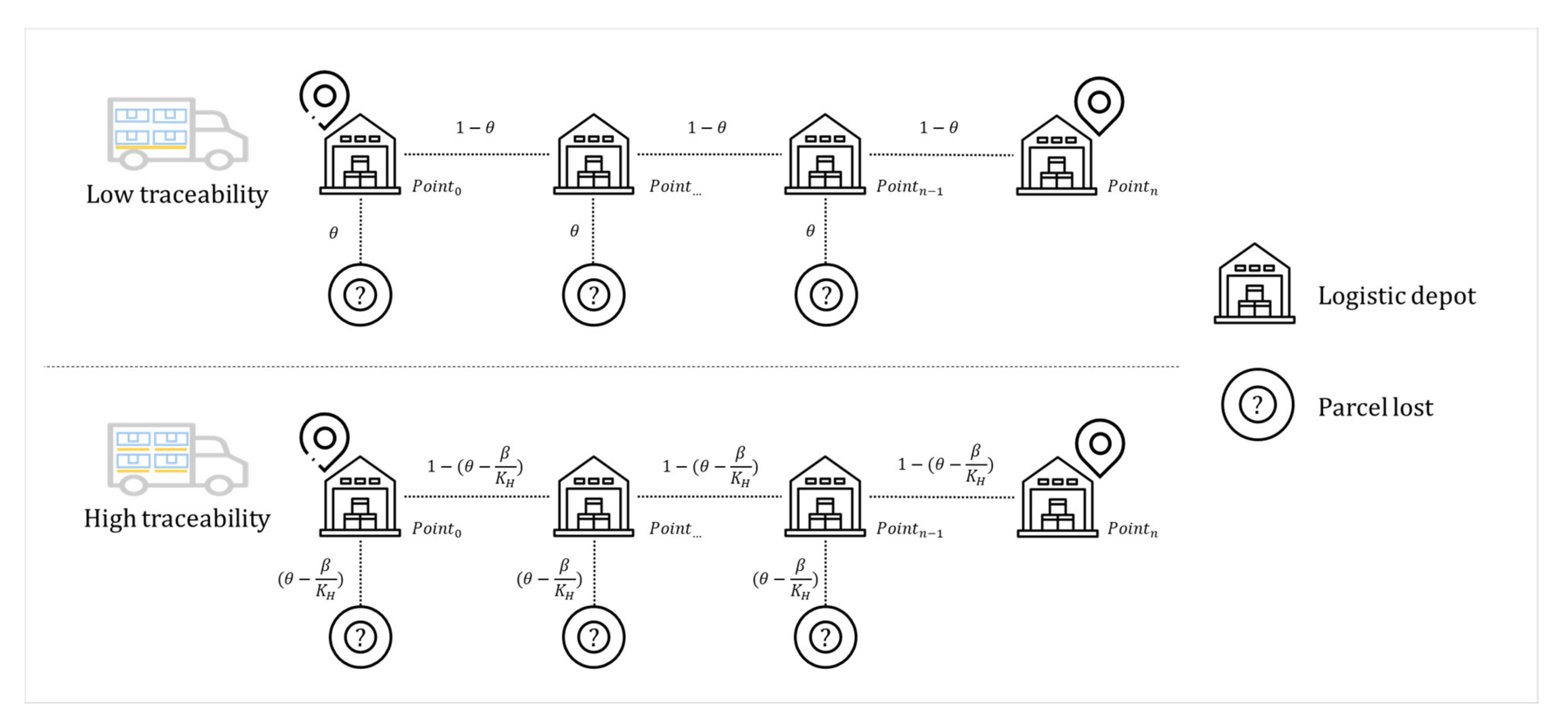
Next, we use a quantitative example to explain how high traceability affects delivery quality. We define the natural probability of the misplacement/damage/loss at one logistics depot as $\theta$. The freight will pass $n$ logistics depots in total. On modeling risk during multi-stage transportation, Erkut et al. [54] noted that the total transport risk shows as the product of the risk rate in all $n$ depots, making the expected probability of freight intact delivered as ${\left(1-\theta \right)}^n$. Therefore, the probability for the freight lost or damaged during the $n$-stage transportation is $1-{\left(1-\theta \right)}^n$. For consistency, we use “natural failure rate” to represent the probability in the rest of the paper. $k_H$ is the capacity of the smart pallet in the high-traceability system, and the system traceability improves as $k_H$ shrinks. $k_0$ marks the smallest traceable unit in basic service (e.g., $k_0$ means the capacity of a truck), and notable, $k_H<k_0$. The smallest traceable capacity $k_0$ incurs a natural failure rate $P^L=\left[1-{\left(1-\mathsf{\theta }\right)}^n\right]$. By introducing the high-traceability system, the probability for the freight lost or damaged in one depot dropping from $\theta$ to $\left(\theta -\beta /k_H\right)$ and the failure rate drops to $P^H=\left[1-{\left(1-\left(\theta -\beta /k_H\right)\right)}^n\right]$, where $\beta$ is a traceability efficiency coefficient. Figure 3 shows how the improved failure rate $P^H$ is calculated. We define ${\tau }_i=1/k_i$, where $i\in \{0, H$}.

3.1. Problem Setting

In this section, we develop a model where the company designs logistics service strategies, which is our benchmark basic service option, and may also introduce a high-traceability logistics service option (by adopting IoT-based tracking system). Two customers segments, namely, TS and TNS customers, are considered. The proportion for TS (TNS) customers in total customers is $n_{TS}$ ($n_{TNS}$) and $n_{TS}+n_{TNS}=1$.

Whether the customers place an order depends on the utility value that they can get from purchasing. We use a linear utility function to model their behavior and preference about price and logistics traceability if they choose basic service:

$$U_i^L=\underset{Expected valuation of receiving product}{\underset{⏟}{\left(1-P^L\right)v}}+\underset{Valuation of logistics traceability}{\underset{⏟}{{\alpha }_i\left({\tau }_0\right)}}-\underset{Product price with free shipping}{\underset{⏟}{r}}+\underset{Compensation}{\underset{⏟}{P^L\lambda r}}, i\in \left\{TS, TNS\right\}$$

for each customer segment, where subscripts $i$ represent TS and TNS customer segments. Parameter $v$ represents the customer’s valuation of receiving the freight (product) when the freight is successfully delivered without loss and damage. The customers’ valuation of logistics traceability ${\alpha }_i\left(·\right)$ measures their additional utility gain from accessing logistics information. TS and TNS customers are heterogeneous in their preference on logistics traceability. TS customers enjoy more benefits from high traceability logistics service than TNS customers. Customers can only recognize the traceability level from the accuracy level of the logistics information that they can access. ${\alpha }_{TS}\left(·\right)$ and ${\alpha }_{TNS}\left(·\right)$ represent the TS and TNS customers’ utility gain from the logistics information and, in this study, have some properties: ${\alpha }_{TS}\left(x\right)\ge {\alpha }_{TNS}\left(x\right)\ge 0$, ${\alpha }_{TS}^{\prime }\left(x\right)\ge {\alpha }_{TNS}^{\prime }\left(x\right)\ge 0$,${\alpha }_{TNS}^{″}\left(x\right)\le {\alpha }_{TS}^{″}\left(x\right)\le 0$. The properties are intuitive as the TS customers value logistics traceability more than TNS, and both segments have a positive utility gain as logistics traceability increases, whereas diminishing the marginal utility is considered.

Any customers who purchase products from the company will be charged a PPFS (the sum of the product price and basic delivery fee) $r$. When the shipment is lost or damaged (with probability $P^L$), the company pays a compensation fee to the customer. We show this amount as a proportion to the price that customers have been charged, and $\mathsf{\lambda }$ is the compensation coefficient.

When high-traceability service is adopted, customer utility function can be written as:

$$U_i^H=\underset{Expected valuation of receiving product}{\underset{⏟}{\left(1-P^H\right)}v}+{\alpha }_i\left({\tau }_H\right)-r-\underset{Value-added service price}{\underset{⏟}{\epsilon }}+\underset{Compensation}{\underset{⏟}{P^H\lambda \left(r+\epsilon \right)}}, i\in \left\{TS, TNS\right\}$$

Table 1. Notations.

Parameters	Meaning
$v$	Freight value
$\theta$	The natural probability of freight loss/damaged in one logistics depot
$\lambda$	The compensation coefficient for delivery failure
$n_i$	The market size of segment $i$, $iϵ\left\{TS,TNS\right\}$
$k_0$	The capacity of the smallest traceable unit when basic service is adopted
${\tau }_0$	Basics logistics traceability level
Decision variables
r	The product price with free shipping (denoted as PPFS) which is the sum of product prices and basic delivery fee
$\epsilon$	The VAS price of high traceability logistics service
$k_H$	The capacity of the smart pallet when high traceability service is adopted
${\tau }_H$	Improved logistics traceability level
Other variables
$U_i^L$	Type $i$ Customers’ utility when choosing basic logistics service, $iϵ\left\{TS,TNS\right\}$
$U_i^H$	Type $i$ Customers’ utility when choosing high-traceability service, $iϵ\left\{TS,TNS\right\}$
$P^j$	The delivery failure rate in the whole delivery process, $j\in \left\{L,H\right\}$
$\Phi$	The operations cost of IoT equipment
${\alpha }_i$	Customers’ additional utility gain from logistics traceability, $iϵ\left\{TS,TNS\right\}$
${\pi }_{\left(A,B\right)}^{*}$	The company’s profit, subscript (A, B) means the services that launched in TNS and TS market segment respectively, $Aϵ\left\{L,H,\varphi \right\}, Bϵ\left\{L,H\right\}$. L/H means low/high traceability, $\varphi$ means the company exits this market segment.
Subscripts
TS	Customers who are sensitive to logistics traceability
TNS	Customers who are not sensitive to logistics traceability

shows the notations that will be frequently used in this study.

3.2. Model Formulation

We consider markets where the company is already present by providing low-traceability service (basic service) to both customer segments (Low-Traceability Strategy, LT), in our model, the company’s IoT adoption pertains to whether it should induce the $\left(H,H\right)$ equilibrium by providing high-traceability service to both customer segments (High-Traceability Strategy, HT),$\left(\varphi ,H\right)$ equilibrium by providing high-traceability service to TS customer segment while exiting the TNS segment (High-end Services Strategy, HES), or $\left(L,H\right)$ equilibrium by providing high-traceability service to the TS customer segment and a low-traceability service to the TNS segment (Differentiated Service Strategy, DS). The four aforementioned IoT adoption strategies differ in the services launching in two customer segments, as shown in

Table 2. IoT Adoption Strategies.

Customer Segment	LT Strategy	HT Strategy	DS Strategy	HES Strategy
TS Customer	Low Traceability	High Traceability	High Traceability	High Traceability
TNS Customer	Low Traceability	High Traceability	Low Traceability	Exit

.

The profit that the company get from providing segment $i$ with low-traceability service at price $r$ is ${\pi }_L=n_i\left(r-P^L\left(\mathsf{\lambda }r+C\right)\right), i\in \left\{TS,TNS\right\}$.

When a low-traceability service is adopted, the delivery failure incurs a communication cost $C$ on the company. The communication cost in our research refers to when delivery failure happens, the company needs to pay for taking a series of actions to resolve the issue, including labor cost to investigate how the loss/damage happened and communicate with the customer. The agent of Amazon or UPS is involved in the complex process of claiming the lost package (e.g., determine the potential value of the lost package, which incurs labor cost). Moreover, the company will pay the compensation according to the ascription of responsibility [55,56], which explains the setting of communication cost $C$ and compensation cost $\mathsf{\lambda }r$ in our model. In addition, when customers complain on social media, the company might suffer from a loss of reputation.

The profit that the company get from providing segment $i$ with high-traceability service at price $r+\epsilon$ is ${\pi }_H=n_i\left(r+\epsilon -\Phi \left({\tau }_H\right)-\lambda P^H\left(r+\epsilon \right)\right), i\in \left\{TS,TNS\right\}$.

Here, the $\Phi \left({\tau }_H\right)$ is the IoT equipment operation cost (e.g., necessary maintenance/replacement cost), which appears as variable expenses. We assume ${\Phi }^{\prime }\left({\tau }_H\right)>0$, and $\epsilon >{\Phi }^{\prime }\left({\tau }_H\right)$ holds for any scenario. Intuitively, the company sets the VAS price higher than the cost for providing this service.

Introducing ${\pi }_L$ and ${\pi }_H$, we next formulate the company’s problem of maximizing the profit from each of $\left(L,L\right)$, $\left(H,H\right)$, $\left(L,H\right)$, and $\left(\varphi ,H\right)$ equilibria. The company knows two customer segments and the preference of each type of customer, whereas individual customers valuation is unobservable to the company. Thus, the company needs to maximize its profit subject to customers’ individual rationality constraints and incentive compatibility constraints under each equilibrium. Therefore, the customers will self-select into the market equilibrium.

3.2.1. Low-Traceability Strategy (LT)

When the company implements the LT strategy, low-traceability services are launched in TS and TNS segments. In particular, the company calculates the price $r^{*}$ that induces both segments to choose low-traceability service over choose nothing (leave the system):

$${\pi }_{\left(L,L\right)}^{*}\left(r\right)= \max \left\{r-P^L\left(\lambda r+C\right)\right\}$$

(1)

$$s.t. \left(1-P^L\right)v+{\alpha }_{TS}\left({\tau }_0\right)-r+P^L\lambda r\ge 0 \left(I{R}_L^{TS}\right)$$

(2)

$$\left(1-P^L\right)v+{\alpha }_{TNS}\left({\tau }_0\right)-r+P^L\lambda r\ge 0 \left(I{R}_L^{TNS}\right)$$

(3)

The individual rationality constraints $I{R}_L^{TS}$ and $I{R}_L^{TS}$ ensure that the two segments benefit from choosing low-traceability services. We consider this situation as the base business model because it has been widely adopted in industry practice. These conditions will align with the strategic intent of the company to guide specific types of customers to choose the appropriate service.

3.2.2. High-Traceability Strategy (HT)

When the company implements the HT strategy, the company launches high-traceability services in TS and TNS segments. In particular, the company determines the PPFS $r^{*}$, VAS price ${\epsilon }^{*}$, and high-traceability level ${\tau }_H$ that induces both segments to choose high-traceability service over choose nothing (leave the system):

$${\pi }_{\left(H,H\right)}^{*}\left(r,\epsilon , {\tau }_H\right)= \max \left\{r+\epsilon -\Phi \left({\tau }_H\right)-\lambda P^H\left(r+\epsilon \right)\right\}$$

(4)

$$s.t. \left(1-P^H\right)v+{\alpha }_{TS}\left({\tau }_H\right)-r-\epsilon +P^H\lambda \left(r+\epsilon \right)\ge 0 \left(I{R}_H^{TS}\right)$$

(5)

$$\left(1-P^H\right)v+{\alpha }_{TNS}\left({\tau }_H\right)-r-\epsilon +P^H\lambda \left(r+\epsilon \right)\ge 0 \left(I{R}_H^{TNS}\right)$$

(6)

The individual rationality constraint $I{R}_H^{TS}$ and $I{R}_H^{TNS}$ ensure that the two segments benefit from choosing high-traceability services.

3.2.3. Differentiated Service Strategy (DS)

In the DS strategy, the company launches high-traceability services in the TS segment while launching low-traceability services in the TNS segment. The company determines the PPFS $r^{*}$, VAS price ${\epsilon }^{*}$, and high-traceability level ${\tau }_H$ to induce TS segment to choose high-traceability service and TNS segment to choose low-traceability service, respectively:

$${\pi }_{\left(L,H\right)}^{*}\left(r,\epsilon , {\tau }_H\right)=\max \left\{n_{TS}\left[r+\epsilon -\Phi \left({\tau }_H\right)-\lambda P^H\left(r+\epsilon \right)\right]+n_{TNS}\left[r-P^L\left(\lambda \mathrm{r}+C\right)\right]\right\}$$

(7)

$$\hspace{0.17em}s.t. \left(1-P^H\right)v+{\alpha }_{TS}\left({\tau }_H\right)-r-\epsilon +P^H\lambda \left(r+\epsilon \right)\ge 0 \left(I{R}_H^{TS}\right)$$

(8)

$$\left(1-P^L\right)v+{\alpha }_{TNS}\left({\tau }_0\right)-r+P^L\lambda r\ge 0 \left(I{R}_L^{TNS}\right)$$

(9)

$$\left(1-P^H\right)v+{\alpha }_{TS}\left({\tau }_H\right)-r-\epsilon +P^H\lambda \left(r+\epsilon \right)\ge \left(1-P^L\right)\mathrm{v}+{\alpha }_{TS}\left({\tau }_0\right)-r+P^L\lambda r \left(I{C}_H^{TS}\right)$$

(10)

$$\left(1-P^L\right)v+{\alpha }_{TNS}\left({\tau }_0\right)-r+P^L\lambda r\ge \left(1-P^H\right)\mathrm{v}+{\alpha }_{TNS}\left({\tau }_H\right)-r-\epsilon +P^H\lambda \left(r+\epsilon \right) \left(I{C}_L^{TNS}\right)$$

(11)

The individual rationality constraint $I{R}_H^{TS}$ and $I{R}_L^{TNS}$ ensure that TS and TNS segments benefit from choosing high-/low-traceability services, respectively. The incentive compatibility constraint $I{C}_H^{TS}$ and $I{C}_L^{TNS}$ ensure that the TS segment prefers high traceability more than low traceability, whereas the TNS segment prefers low over high traceability, respectively.

3.2.4. High-End Service Strategy (HES)

In the HES strategy, the company exits the TNS segment and only serves the TS customers with high-traceability services. The company determines the PPFS $r^{*}$, VAS price ${\epsilon }^{*}$, and high-traceability level ${\tau }_H$ to induce TS segment to choose high-traceability service and TNS segment to choose nothing (leave the system):

$${\pi }_{\left(\varphi ,H\right)}^{*}\left(r,\epsilon , {\tau }_H\right)=\max n_{TS}\left\{r+\epsilon -\Phi \left({\tau }_H\right)-\lambda P^H\left(r+\epsilon \right)\right\}$$

(12)

$$s.t. \left(1-P^H\right)v+{\alpha }_{TS}\left({\tau }_H\right)-r-\epsilon +P^H\lambda \left(r+\epsilon \right)\ge 0 \left(I{R}_H^{TS}\right)$$

(13)

$$\left(1-P^H\right)v+{\alpha }_{TNS}\left({\tau }_H\right)-r-\epsilon +P^H\lambda \left(r+\epsilon \right)<0 \left(I{R}_{\varphi }^{TNS}\right)$$

(14)

In the next section, we will characterize the company’s optimal decision under each IoT adoption strategy. We will start by investigating how poor delivery quality will affect the company business and analyze the company’s pricing decision and high-traceability level selection in the later part. We prove that the optimization of pricing decisions and high-traceability level selection can be handled separately. Notably, when solving the company optimization problem, different IR and IC constraints can bind at optimality in each case.

4. Pricing Decision and IoT Adoption Decision

In this section, we will discuss the company’s pricing decision and IoT adoption decision. We will derive the analytical results for the proposed models and provide proof.

Lemma 1.

The company have the incentive to at least control the failure rate in delivery where $P^L<1/\lambda$to avoid a deficit. Otherwise, the company needs to pay a subsidy to customers to induce them to place orders.

Proof. 

Please refer to Appendix A. □

Lemma 1 shows that our model captures the characteristic that the company has sufficient incentive to reduce the delivery failure rate. When freight loss happens frequently, the company’s reputation will be affected negatively. The company cannot get profit from the market by setting a regular price because customers do not trust the company’s delivery quality and refuse to place an order. The company has to offer customers subsidies (set price $r<0$) to induce customers to purchase on the website; otherwise, the company will be forced out of the market. The benefit for the company will be twofold if the company manages to reduce the failure rate until $P^L<1/\mathsf{\lambda }$. The company can set a positive optimal PPFS and also increase the guaranteed compensation rate to advertise their logistics service. A highly guaranteed compensation rate will convince the customers that the company can provide a high-quality delivery service.

Proposition 1.

When the company manage to reduce the failure rate in delivery ($P^L<1/\lambda$), the optimal product price with free shipping: $r^{*}=\frac{\left(1-P^L\right)v+{\alpha }_{TNS}\left({\tau }_0\right)}{1-\lambda P^L}$, additionally, $\frac{\partial r^{*}}{\partial v}>0$,$\frac{\partial r^{*}}{\partial \lambda }>0$.

Proof. 

Please refer to Appendix A. □

As shown in Proposition 1, the optimal PPFS directly shows customers’ WTP for the product-delivery service bundle. The delivery service includes fragmented logistics information. We found that the customers’ WTP for logistics information availability is moderated by the delivery quality (information availability, $A={\alpha }_{TNS}\left({\tau }_0\right)/\left(1-\lambda P^L\right)$). In certain situations, for example, $\partial A/\partial {\tau }_0>0$, when the delivery quality is poor, customers value logistics information availability more because logistics information can help them rebuild their confidence in delivery quality. Besides, the company can enhance customer confidence by providing a higher compensation rate ($B=\left(\left(1-P^L\right)/\left(1-\lambda P^L\right)\right)v$, $\partial B/\partial \lambda >0$).

To facilitate the illustration, we define three new symbols to measure how customers utility change as the traceability level changes: ${\Delta }_{TS}={\alpha }_{TS}\left({\tau }_H\right)-{\alpha }_{TS}\left({\tau }_0\right)$, ${\Delta }_{TNS}={\alpha }_{TNS}\left({\tau }_H\right)-{\alpha }_{TNS}\left({\tau }_0\right)$ are the TS/TNS customers’ utility gain when logistics traceability improves, respectively, where ${\Delta }_{TS}\ge {\Delta }_{TNS}\ge 0$. ${\Delta }_{TNS}^{TS}\left(·\right)={\alpha }_{TS}\left(·\right)-{\alpha }_{TNS}\left(·\right)$ is the utility gap between TS and TNS customers under the same traceability level, where ${\Delta }_{TNS}^{TS}\left({\tau }_H\right)={\alpha }_{TS}\left({\tau }_H\right)-{\alpha }_{TNS}\left({\tau }_H\right)$, ${\Delta }_{TNS}^{TS}\left({\tau }_0\right)={\alpha }_{TS}\left({\tau }_0\right)-{\alpha }_{TNS}\left({\tau }_0\right)$, ${\Delta }_{TNS}^{TS}\left({\tau }_H\right)\ge {\Delta }_{TNS}^{TS}\left({\tau }_0\right)\ge 0$.

Next, we will show a finding on the VAS pricing decisions:

Proposition 2.

The company’s optimal product price with free shipping and VAS price: $r_{DS}^{*}=r_{LT}^{*}=\frac{\left(1-P^L\right)v+{\alpha }_{TNS}\left({\tau }_0\right)}{1-\lambda P^L}$; ${\epsilon }_{HT}^{*}=\frac{\left(1-P^H\right)v+{\alpha }_{TNS}\left({\tau }_H\right)}{1-\lambda P^H}-r$, additionally, $\frac{\partial {\epsilon }_{HT}^{*}}{\partial v}>0$, $\frac{\partial {\epsilon }_{HT}^{*}}{\partial \lambda }>0$, $\frac{\partial {\epsilon }_{HT}^{*}}{\partial r}<0$; ${\epsilon }_{DS}^{*}=\frac{{\Delta }_{TS}- \left(P^L-P^H\right)\left(\lambda r-v\right)}{1-\lambda P^H}$, additionally, $\frac{\partial {\epsilon }_{DS}^{*}}{\partial r}<0$; ${\epsilon }_{HES}^{*}=\frac{\left(1-P^H\right)v+{\alpha }_{TS}\left({\tau }_H\right)}{1-\lambda P^H}-r$, additionally, $\frac{\partial {\epsilon }_{HES}^{*}}{\partial v}>0$, $\frac{\partial {\epsilon }_{HES}^{*}}{\partial \lambda }>0$, $\frac{\partial {\epsilon }_{HES}^{*}}{\partial r}<0$.

Proof. 

Please refer to Appendix A. □

We derive the optimal VAS price under different IoT adoption strategies. We found that a higher value freight will enhance customers’ WTP for higher-quality delivery, which is intuitive. The customers would like to pay more to ensure that they can receive their treasurable freight in good condition. In addition, in HT and HES strategies, a higher compensation rate helps to push up VAS prices. The compensation rate shows the company’s confidence in its logistics fulfillment capability, which in turn makes customers feel it noteworthy to pay more for the improved delivery quality. However, in the DS strategy, the relationship between VAS price and compensation is not monotonous, which depends on multiple factors.

For optimal VAS price under the DS strategy, ${\epsilon }_{DS}^{*}$, we found that VAS in the DS strategy might be profitable only when TS customers’ utility gain ${\Delta }_{TS}$ is higher than the company’s compensation cost saving from the updating system. As we mark below, the $\left(P^L-P^H\right)$ is the improvement of the delivery failure rate, $\left(\lambda r-v\right)$ is the compensation cost for basic logistics service (which is calculated by the company’s total compensation cost $\lambda r$ minus the product value $v$). The company cannot profit from VAS when the above condition does not hold (${\epsilon }_{DS}^{*}<0$). The reason is that customers’ utility can sufficiently improve only in the high-traceability logistics service (including real-time logistics information); otherwise, even the TS customers do not have the incentive to switch from a basic service to a high-traceability service.

$${\Delta }_{TS}> \underset{Failure rate improvement}{\underset{⏟}{\left(P^L-P^H\right)}}\bullet \underset{Compensation for poor service}{\underset{⏟}{\left(\lambda r-v\right)}}$$

We also found that a substitution relationship exists between optimal VAS price and PPFS, which will be addressed in Corollary 1.

Corollary 1.

The relationship between optimal product price with free shipping and VAS price shows as $-1=\frac{\partial {\epsilon }_{HT}^{*}}{\partial r}=\frac{\partial {\epsilon }_{HES}^{*}}{\partial r}<\frac{\partial {\epsilon }_{DS}^{*}}{\partial r}<0$.

Proof. 

Please refer to Appendix A. □

Under HT and HES strategies, the marginal rate of substitution between optimal VAS price and PPFS is equal to $-1$, which means that the two kinds of charges are perfect substitution. In these two situations, the product and high-traceability logistics are provided as a bundle, where customers only care about the total price rather than distinguish which part of the price is for the product or service.

However, under the DS strategy, the marginal rate of substitution $-1<\partial {\epsilon }_{DS}^{*}/\partial r<0$, which indicates that raising the PPFS can achieve Pareto optimality; thus, the company will set the PPFS exactly binding at optimality ($r^{*}=\frac{\left(1-P^L\right)v+{\alpha }_{TNS}\left({\tau }_0\right)}{1-\lambda P^L}$). The reason for the Pareto improvement is that the company uses the PPFS to take TNS customer’s “consumer surplus,” and they will set the price as high as possible.

We continue by analyzing the relationship between optimal VAS prices under different IoT adoption strategies. Here, we assume that ${\tau }_H$ are identical in different strategies:

Proposition 3.

The relationship of optimal VAS price under different strategies when identical product price with free shipping and high-traceability solution is adopted:

(1) 

${\epsilon }_{HES}^{*}\ge {\epsilon }_{HT}^{*}$and${\epsilon }_{HES}^{*}\ge {\epsilon }_{DS}^{*}$ hold at all conditions.

(2) 

${\epsilon }_{HES}^{*}\ge {\epsilon }_{DS}^{*}\ge {\epsilon }_{HT}^{*}$holds when the company sets product price with free shipping$r\ge \frac{\left(1-P^L\right)v-{\Delta }_{TS}+{\alpha }_{TNS}\left({\tau }_H\right)}{1-\lambda P^L}.$

(3) 

${\epsilon }_{DS}^{*}<{\epsilon }_{HT}^{*}$holds when the company adopts identical product price with free shipping$r<\frac{\left(1-P^L\right)v-{\Delta }_{TS}+{\alpha }_{TNS}\left({\tau }_H\right)}{1-\lambda P^L}$, the HT strategy is more profitable than the DS strategy.

Proof. 

Please refer to Appendix A. □

Proposition 3 shows the fundamental principle of how different high-traceability adoption strategies (HT, DS, HES) maximize the company’s profitability. In the HT strategy, the company expands the market and attracts customers who are seeking high-traceability logistics services. The company uses VAS to take more TS customers’ consumer surplus, which is more profitable for the company than adopting the LT strategy. However, TNS customers’ financial capability limits the upper bound of ${\epsilon }_{HT}^{*}$. Therefore, the HT strategy is a strategy that the company would like to improve service quality and optimize customers’ experience while charging a relatively low price.

The DS strategy separates two customer segments. Their company serves the TNS segment with basic service while offering high-traceability service to the TS segment. Then, the pricing of VAS is no longer restricted by TNS customers’ financial capacity. We found that as the PPFS increases, the relationship between the two VAS prices switches from ${\epsilon }_{DS}^{*}<{\epsilon }_{HT}^{*}$ to ${\epsilon }_{DS}^{*}\ge {\epsilon }_{HT}^{*}$. Notably, when ${\epsilon }_{DS}^{*}<{\epsilon }_{HT}^{*}$, the setting of the DS strategy is not Pareto optimal, and the HT strategy is more profitable than the DS strategy. The advantage of the DS strategy is that it grants the company the ability to separate different customers, improves VAS price, and then takes more TS customers’ consumer surplus. When that advantage cannot be achieved, the DS strategy cannot outperform HT strategy.

In the HES strategy, the company gives up the TNS segment. Therefore, the upper limit of ${\epsilon }_{HES}^{*}$ further improves, the company takes all the TS customers’ consumer surplus to offset the loss of exiting the TNS market. In this strategy, intuitively, the company will set a highest ${\epsilon }^{*}$ compared with pricing decisions in other strategies. As we demonstrate in Proposition 3(1) the ${\epsilon }_{HES}^{*}$ is the highest VAS price, which always holds.

At the end of this section, we will explain why we can optimize the company’s price decision and traceability level decision separately.

Proposition 4.

(1) 

For a giventraceability (${\tau }_0$), only one optimalVASprice$r^{*}$exists that optimizes the company’s profit under the LT strategy.

(2) 

For a given group of traceability and product price with free shipping (${\tau }_0,{\tau }_H,r$), only one optimal VAS price${\epsilon }^{*}$exists that optimizes the company’s profit under HT, DS, and HES strategies, respectively.

Proof. 

Please refer to Appendix A. □

As shown in Proposition 4, when the traceability level (${\tau }_0,{\tau }_H$) are given, unique optimal pricing decision always exists. Therefore, the optimization of price and traceability level can be handled separately. We will further analyze how the choice of traceability level affects the performance of each IoT adoption decision.

After deriving some findings of optimal pricing under each strategy, we start to explore the appropriate market condition for each strategy. We will also clarify the corresponding environment for each strategy to be optimal.

4.1. Optimal Profit of HT, LT, DS, and HES Strategies

By solving the company’s optimization problem, we derive the company’s optimal profit under promoted IoT adoption strategies, please refer to Appendix A-Proof for Proposition 5 for more details.

$${\pi }_{\left(L,L\right)}^{*}=\left(1-P^L\right)v+{\alpha }_{TNS}\left({\tau }_0\right)-C{P}^L$$

$${\pi }_{\left(H,H\right)}^{*}=\left(1-P^H\right)v+{\alpha }_{TNS}\left({\tau }_H\right)-\Phi \left({\tau }_H\right)$$

$${\pi }_{\left(L,H\right)}^{*}=\left(1-P^L\right)v+{\alpha }_{TNS}\left({\tau }_0\right)+ n_{TS}\left[{\Delta }_{TS}+\left(P^L-P^H\right)v-\Phi \left({\tau }_H\right)\right]-n_{TNS}C{P}^L$$

$${\pi }_{\left(\varphi ,H\right)}^{*}=n_{TS}\left[\left(1-P^H\right)v+{\alpha }_{TS}\left({\tau }_H\right)-\Phi \left({\tau }_H\right)\right]$$

Based on the above equation, we found that the optimal profit under each strategy directly shows the market potential. The value of freight and customers’ utility gain from logistics traceability contributes to the company’s profitability, which precisely illustrates the industry practice we want to model. As the traceability increases, the company’s revenue increases, however, high operation cost also incurs. The quality gap between high-traceability service and basic service is the source of profit under the DS strategy. In HT, DS, and HES strategies, the company needs to decide the optimal traceability level that maximizes profit. We give a finding of the company’s decision on high-traceability level selection:

Proposition 5.

The optimal high-traceability level in DS and HES strategies is identical ${\tau }_{H\_1}$, and the optimal traceability level in HT strategy satisfies ${\tau }_{H\_2}\le {\tau }_{H\_1}$.

Proof. 

Please refer to Appendix A. □

The DS and HES grant the company the capability to serve the TS segment with a higher traceability level than that in the HT strategy. This finding is not counter-intuitive, and the high traceability in the HT strategy is more like one kind of “social public product.” Moreover, the company does its best to improve the delivery quality in all segments on the premise of not losing money. We discuss in the previous part that the VAS price in the HT strategy is restricted by the financial capability of TNS customers. Thus, the HT might be considered a strategy that is good for the public.

Next, we will study a different situation where the traceability level (${\tau }_H$) is an exogenous variable rather than a decision variable. The traceability level may not be fully controllable, where the company cannot set it at the theoretical optimal point in practice. For example, a company adopts the supplier’s IoT solutions where the performance of the introduced tracking system is bounded. In such circumstances, the traceability level (${\tau }_H$) is identical among all strategies.

4.2. IoT Adoption Decisions

To explore the connection between the market condition and the company’s optimal IoT adoption decision, we summarize how the company’s optimal choice evolves as the market condition changes. Market conditions that we focus on include communication cost for solving delivery failure, and IoT equipment operations cost.

Proposition 6.

Two optimal strategy transfer paths exist:

(1) 

When the companies’ communication cost (when freight loss or damaged) is$C<C_1$, as the IoT equipment operation cost increases, the optimal strategy switches from HT → DS → LT.

(2) 

When the companies’ communication cost (when freight loss or damaged) is$C\ge C_1$, as the IoT equipment operation cost increases, the optimal strategy switches from HT → HES → LT.

Table 3. Optimal Strategy Transfer Paths.

	$\mathit{C}<{\mathit{C}}_{\mathbf{1}}$	$\mathit{C}\ge {\mathit{C}}_{\mathbf{1}}$
$\mathit{\Phi }\left({\mathit{\tau }}_{\mathit{H}}\right)\le {\mathit{\Phi }}_{\mathit{2}}$	HT
${\mathit{\Phi }}_{\mathit{2}}\le \mathit{\Phi }\left({\mathit{\tau }}_{\mathit{H}}\right)\le {\mathit{\Phi }}_{\mathit{4}}$	DS
$\mathit{\Phi }\left({\mathit{\tau }}_{\mathit{H}}\right)\ge {\mathit{\Phi }}_{\mathit{4}}$	LT
$\mathit{\Phi }\left({\mathit{\tau }}_{\mathit{H}}\right)\le {\mathit{\Phi }}_{\mathit{3}}$		HT
${\mathit{\Phi }}_3\le \mathit{\Phi }\left({\tau }_{\mathit{H}}\right)\le {\mathit{\Phi }}_{\mathit{5}}$		HES
$\mathit{\Phi }\left({\mathit{\tau }}_{\mathit{H}}\right)\ge {\mathit{\Phi }}_{\mathit{5}}$		LT

shows the detail.

Proof. 

Please refer to Appendix A. □

From Proposition 6, we verified the validity of an intuitive conjecture. That is, as IoT equipment operation costs increase, the optimal strategy switches from HT to LT strategy. The HT strategy is only feasible when the operation cost is low. Moreover, as the HT strategy is providing a “public product”, the pricing decision under this strategy is restricted by TNS customers’ financial capacity. Therefore, the HT strategy cannot hedge high IoT operation costs by adopting a high VAS price.

The DS strategy is effective when IoT operations cost is neither too high nor too low. As we discussed in the previous part, the DS strategy successfully separates two segments, and the high revenue earned from the TS segment can partially mitigate the IoT operation cost. However, as IoT operation cost keeps increasing, the DS strategy does not work either.

Providing high-traceability logistics service when IoT operations cost is high is uneconomic. Thus, only the LT strategy can be adopted, which means that the company should not upgrade its system. In this case, for example, the IoT equipment might not be very durable, and the company needs to keep repairing or replacing it. In such a situation, the company has to carefully choose the IoT supplier and avoid unreliable hardware. Then, the HT or DS strategy could be viable.

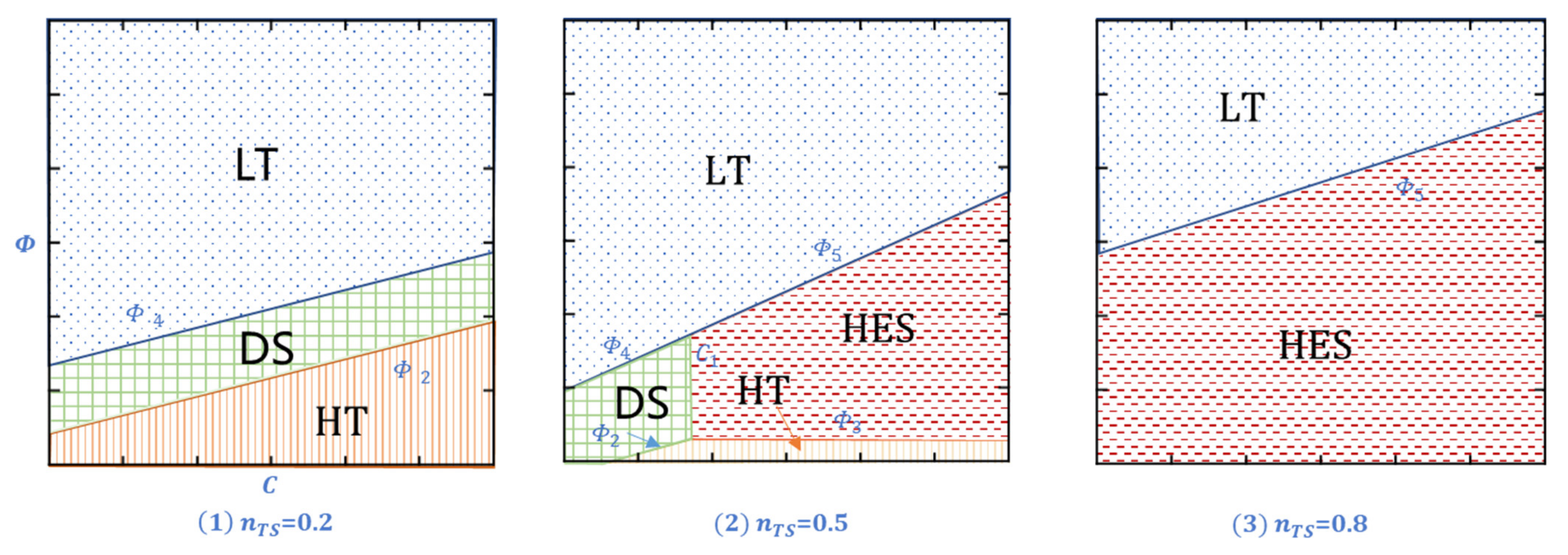
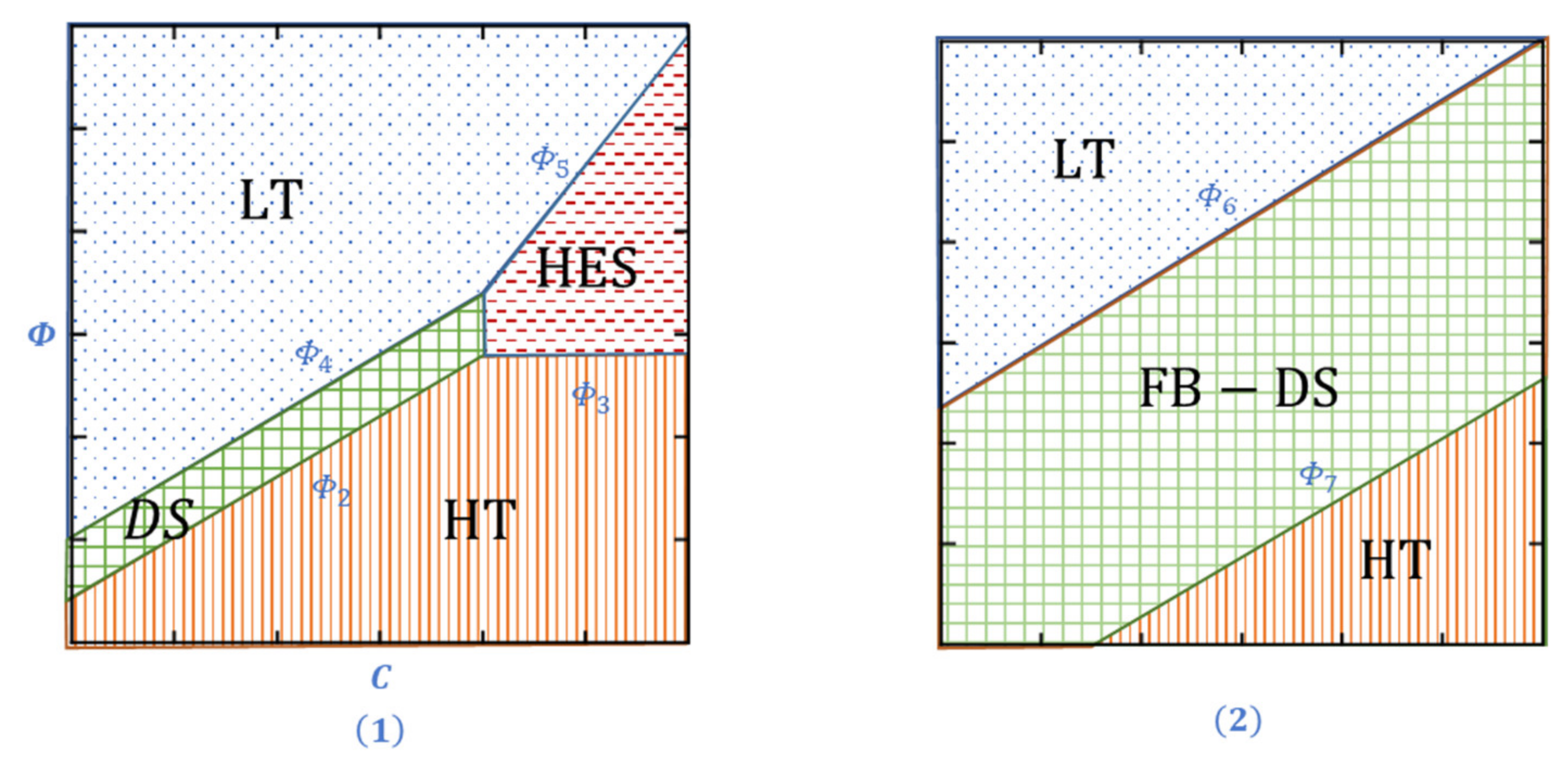
As mentioned above, the DS strategy is an intuitive middle choice for the company to offer differentiated service to two segments, which appears at an intermediate state from the HT to LT strategy. However, Proposition 6 shows us another situation, when the communication cost of the company is high ($C\ge C_1$), the optimal strategy still switches from HT to LT, whereas the HES strategy replaces the DS strategy as an optimal middle option. Unintuitively, HES acts as a middle option between HT and LT strategies, as the HES is an aggressive strategy itself. The HES strategy encourages the company to completely abandon the TNS market and only serve the TS segment with high-traceability service. This situation happens for two reasons; one is that the TS customers are considered as “high net worth clients”, exits the TNS segment allows the company to set a VAS price that exactly binds at TS customer’s total budget. By taking TS customers’ “consumer surplus”, the company maximizes its profit. Another reason is that the TS segment occupies a relatively big share of the total market. The proof is that, $\partial {\Phi }_3/\partial n_{TS}<0$ and $\partial {\Phi }_5/\partial n_{TS}>0$, where as the share of TS segment $n_{TS}$ expands, the region for the HES strategy to be an optimal option also expands. Figure 4 shows that when the TS segment is small, HES is excluded from the optimal strategy set. As the TS segment expands, the HES appears as an optimal strategy when $C\ge C_1$ ($\partial C_1/\partial n_{TS}<0$). When TS share is at a high position, only LT and HES are left in the optimal strategy set.

In the previous discussion, the performance of the DS strategy is affected by information asymmetry. The company cannot realize the first-best pricing decision because the company needs to introduce IC constraints for each segment and information rent is incurred. We would like to further explore information asymmetry’s impact on the DS strategy.

4.2.1. Differentiated Service Strategy (DS) under full information

We will analyze the first best solution of the DS strategy, which shows the profit upper bound of DS strategy under asymmetric information. The company knows exactly each customers’ type under full information situation; therefore, the company serves the customer with the unique selected option according to their type (and the rest option is invisible to the customer). The customers either place the order or leave it. The company optimization problem is shown as follows:

$${\pi }_{\left(L,H\right)}^{FB}\left(r,\epsilon \right)=\max \left\{n_{TS}\left[r+\epsilon -\Phi \left({\tau }_H\right)-\lambda P^H\left(r+\epsilon \right)\right]+n_{TNS}\left[r-P^L\left(\lambda \mathrm{r}+C\right)\right]\right\}$$

(15)

$$\hspace{0.17em}s.t. \left(1-P^H\right)v+{\alpha }_{TS}\left({\tau }_H\right)-r-\epsilon +P^H\lambda \left(r+\epsilon \right)\ge 0 (I{R}_H^{TS})$$

(16)

$$\left(1-P^L\right)v+{\alpha }_{TNS}\left({\tau }_0\right)-r+P^L\lambda r\ge 0 \left(I{R}_L^{TNS}\right)$$

(17)

In such a case, the IR condition for the customer is binding at optimality, whereas the IC constraint is redundant (we drop that from the model). Hence, the PPFS is $r_{DS-FB}^{*}=\frac{\left(1-P^L\right)v+{\alpha }_{TNS}\left({\tau }_0\right)}{1-\lambda P^L}$, and the VAS price is ${\epsilon }_{DS-FB}^{*}=\frac{\left(1-P^H\right)v+{\alpha }_{TS}\left({\tau }_H\right)}{1-\lambda P^H}-r$.

The optimal profit under the DS strategy with full information ${\pi }_{\left(L,H\right)}^{FB}$ shows the following:

$${\pi }_{\left(L,H\right)}^{FB}=n_{TS}\left(\left(1-P^H\right)v+{\alpha }_{TS}\left({\tau }_H\right)-\Phi \left({\tau }_H\right)\right)+n_{TNS}\left(\left(1-P^L\right)v+{\alpha }_{TNS}\left({\tau }_0\right)-C{P}_L\right)$$

By analyzing the DS strategy with full information, we found the following:

Proposition 7.

The company’s optimal decision and optimal profit:

(1) 

$r_{DS-FB}^{*}=r_{DS}^{*}=\frac{\left(1-P^L\right)v+{\alpha }_{TNS}\left({\tau }_0\right)}{1-\lambda P^L}$.

(2) 

${\epsilon }_{DS-FB}^{*}={\epsilon }_{HES}^{*}=\frac{\left(1-P^H\right)v+{\alpha }_{TS}\left({\tau }_H\right)}{1-\lambda P^H}-r$, ${\epsilon }_{DS-FB}^{*}\ge {\epsilon }_{DS}^{*}.$

(3) 

${\tau }_H^{*}={\tau }_{H\_1}$.

(4) 

Theprofit gap between the DS strategy with or without full information is$G=n_{TS}{\Delta }_{TNS}^{TS}\left({\tau }_0\right)$.

(5) 

The DS strategy with full information dominates the HES strategy at any condition.

(6) 

When  $\Phi \left({\tau }_H\right)\le {\Phi }_6$, the DS strategy outperforms LT strategy, where the  ${\Phi }_6\ge {\Phi }_4.$

(7) 

When traceability level  ${\tau }_H$is fixed, and  $\Phi \left({\tau }_H\right)\ge {\Phi }_7$  ,the DS strategy with full information outperforms HT strategies, where  ${\Phi }_7\le {\Phi }_2.$

Proof. 

Please refer to Appendix A. □

The superiority of full information is significant, and the DS strategy eliminates information rent paid to incentive customers self-selected to their desired services, and the VAS price exactly sets the same level as in the HES strategy. Benefiting from such effect, the full information DS strategy dominates the DS under information asymmetry (and HES strategy). The profit gap $G$ (also refers to information cost) increases with a valuable difference for basic traceability level (${\tau }_0$) between two customers types. This finding implies that the information cost increases as TS customers valuation for the traceability level in basic service ${\alpha }_{TS}\left({\tau }_0\right)$ increases. As we mentioned in the Proof for Proposition 2, the IC constraint for TS customers is binding at optimality. To attract TS customers to abandon basic service and turn to high-traceability service, the company has to concede on VAS price. Therefore, the information cost will be high when TS customers value the traceability level in basic service a lot which indicates that DS is hard to separate two segments. Similarly, when the market share of TS segment ($n_{TS}$) increases, the information cost also increases. The company might lose more potential gains when they need to provide incentives to a larger part of TS customers.

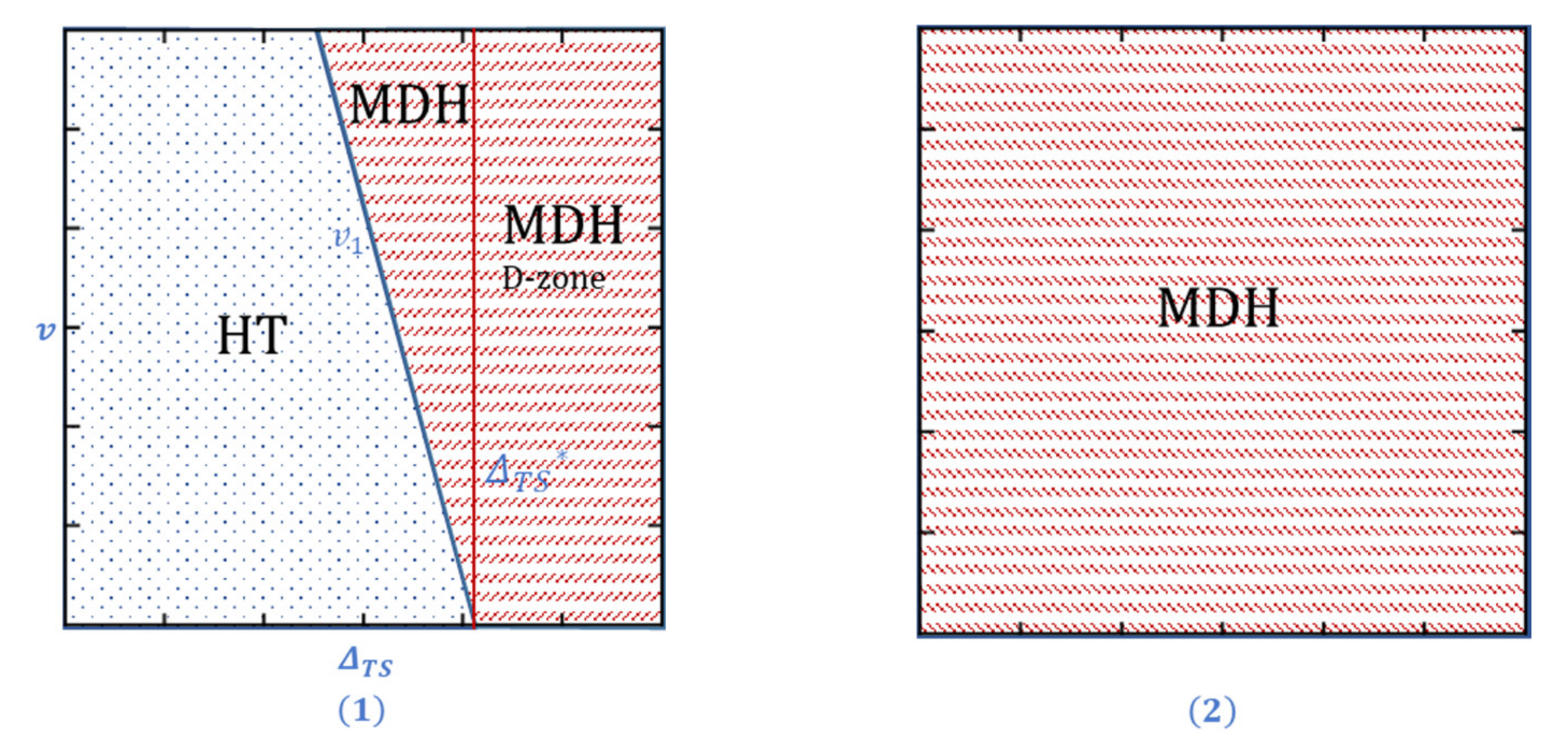
The DS strategy with full information also shows superiority that it can sustain under higher IoT operation costs. As we mentioned in Proposition 6, the DS strategy becomes optimal when ${\Phi }_2\le \Phi \left({\tau }_H\right)\le {\Phi }_4$ (when $C\le C_1$ holds). In the DS with full information, the threshold for $\Phi \left({\tau }_H\right)$ is $\left[{\Phi }_7,{\Phi }_6\right]$, which indicates that the range for the DS strategy to be optimal strategy is enlarged (${\Phi }_7\le {\Phi }_2$, ${\Phi }_6\ge {\Phi }_4$). Figure 5 shows that when the full information DS (FB-DS) is introduced, it dominates DS, HES, and even a part of a region previously occupied by HT and LT. In the meanwhile, we found that information advantage will not change the company’s pricing decision $r$ and traceability level decision, and the $r^{*}$ and ${\tau }_H^{*}$ is identical in full information case or information asymmetric case.

The high-traceability service affects the company’s profit from two aspects, one is fulfilling customers’ demand on logistics traceability, and the other is reducing the delivery failure rate. To better understand the tradeoff, we conduct the following analysis to isolate two kinds of effects. Except for the four strategies promoted above, the company could adopt a Mix DS-HT strategy, that is, the company adopts a high-traceability technology in both segments but will still provide differentiated accuracy logistics information. Customers who choose the basic services will not recognize that their delivery failure rate is $P^H$ rather than $P^L$ as the company only offers fragmented logistics information. The company still charges TNS customers for the basic service fee but might benefit from a reduced delivery failure rate.

4.2.2. Mix DS-HT Strategy (MDH)

We denote the company’s profit under the Mix DS-HT strategy as ${\pi }_{\left(LH,H\right)}$:

$${\pi }_{\left(LH,H\right)}^{*}=\max \left\{n_{TS}\left\{r+\epsilon -\Phi \left({\tau }_H\right)-\lambda P^H\left(r+\epsilon \right)\right\}+n_{TNS}\left[r-\Phi \left({\tau }_H\right)-\lambda P^H\mathrm{r}\right]\right\}\hspace{0.17em}\mathrm{s}.\mathrm{t}.I{R}_H^{TS}, I{R}_L^{TNS}, I{C}_H^{TS}, I{C}_L^{TNS}$$

(18)

In MDH, the company reduces the overall failure rate by adopting IoT technology. The disclosure of real-time logistics information becomes the instrument for services differentiation. The company provides real-time logistics information to TS segments and fragmented information to TNS segments, whereas the real delivery failure rates are identical $P^H$.

As MDH is a mixture of HT and DS strategies, we compare the performance of the MDH strategy with HT and DS strategies, respectively, the findings show the following:

Proposition 8.

(1) 

$r_{MDH}^{*}=r_{DS}^{*}=\frac{\left(1-P^L\right)v+{\alpha }_{TNS}\left({\tau }_0\right)}{1-\lambda P^L}$,${\epsilon }_{MDH}^{*}={\epsilon }_{DS}^{*}=\frac{{\Delta }_{TS}-\left(P^L-P^H\right)\left(\lambda r-v\right)}{1-\lambda P^H}$

(2) 

${\pi }_{\left(LH,H\right)}^{*}=n_{TS}{\Delta }_{TS}-\Phi \left({\tau }_H\right)+n_{TS}\left(P^L-P^H\right)v+\frac{1-n_{TS}\lambda P^L-n_{TNS}\lambda P^H}{1-\lambda P^L}\left(\left(1-P^L\right)v+{\alpha }_{TNS}\left({\tau }_0\right)\right)$

(3) 

When$n_{TS}{\Delta }_{TS}\ge X_1$, the MDH strategy dominates the HT strategy at any condition. When$n_{TS}{\Delta }_{TS}<X_1$, the MDH strategy outperforms the HT strategy if the$v\ge \frac{X_1-n_{TS}{\Delta }_{TS}}{Y_1}$. This threshold increases in the TNS customers valuation gain from traceability improvement ${\Delta }_{TNS}$and decreases in TS customers valuation gain from traceability improvement${\Delta }_{TS}$.

(4) 

When$\Phi \left({\tau }_H\right)<X_2$, the MDH strategy dominates the DS strategy at any condition. When$\Phi \left({\tau }_H\right)\ge X_2$, the MDH strategy outperforms the DS strategy if$v\ge \frac{\Phi \left({\tau }_H\right)-X_2}{Y_2}$. This threshold increases in the IoT operation cost$\Phi \left({\tau }_H\right)$, and decreases in communication cost$C$and TNS customer valuation of traceability in basic logistics service${\alpha }_{TNS}\left({\tau }_0\right)$.

Note:$X_1={\alpha }_{TNS}\left({\tau }_H\right)-\frac{1-n_{TS}\lambda P^L-n_{TNS}\lambda P^H}{1-\lambda P^L}{\alpha }_{TNS}\left({\tau }_0\right)\le {\Delta }_{TNS}$, ,$Y_1=\left(1-n_{TS}{P}^L-n_{TNS}{P}^H\right)\left(\frac{\lambda -1}{1-\lambda P^L}\right)P^L$,$X_2=C{P}^L+\lambda \frac{P^L-P^H}{1-\lambda P^L}{\alpha }_{TNS}\left({\tau }_0\right)$,$Y_2=\lambda \frac{P^L-P^H}{1-\lambda P^L}\left(1-P^L\right)$.

Proof. 

Please refer to Appendix A.

When TS customers valuation gain from traceability improvement ${\Delta }_{TS}$ is significantly large compared with TNS customers’ improvement ${\Delta }_{TNS}$, MDH always dominates the HT strategy. That is, whether to launch MDH depends on TS customers’ sensitivity to traceability improvement. However, detecting the TS segment’s WTP for traceability improvement relies on market research. When TS segment’s WTP for traceability improvement is not strong enough, strategy adoption depends on freight value $v$. Moreover, when the freight value is larger than a certain threshold, the MDH is better-off; otherwise, the HT strategy is better-off. The threshold increases in the ${\Delta }_{TNS}$, and decreases in ${\Delta }_{TS}$, which is consistent with the above arguments. That is, a market with extremely traceability sensitive TS segment and extremely traceability not sensitive TNS segment will facilitate the MDH, showing its advantage.

Figure 6(1) shows that when the TS segment is relatively small, the performance of the two strategies depends on ${\Delta }_{TS}$ and $v$. We indicate the MDH domination zone where ${\Delta }_{TS}$ is large enough. However, if ${\Delta }_{TS}$ is at the intermediate level, MDH is only better-off when $v$ is high. The reason is that as the freight value $v$ increases, the TS customers are willing to pay more in exchange for their freight to be delivered safe and sound, which can mitigate a company’s potential profit loss. When the TS segment is large, the MDH dominates the HT strategy (Figure 6(2)).

To summarize, the MDH is proposed based on the idea that the company might reduce the failure rate in both segments and avoid the corresponding cost (including compensation and company internal communication). MDH incurs a profit loss, as it completely upgrades the logistics service but did not charge TNS customers an additional fee. Thus, the company wishes that their TS customers will be excited with traceability improvement and pay enough money (to cover the investment on IoT operation cost in both segments). This case contributes to the company’s generous offering that no additional charge to the TNS segment (TNS customers would not pay more for high traceability anyway). When TS and TNS customers are only slightly different on their valuation gain from traceability improvement, MDH is inappropriate because it incurs large potential profit loss, unless freight value $v$ is high enough.

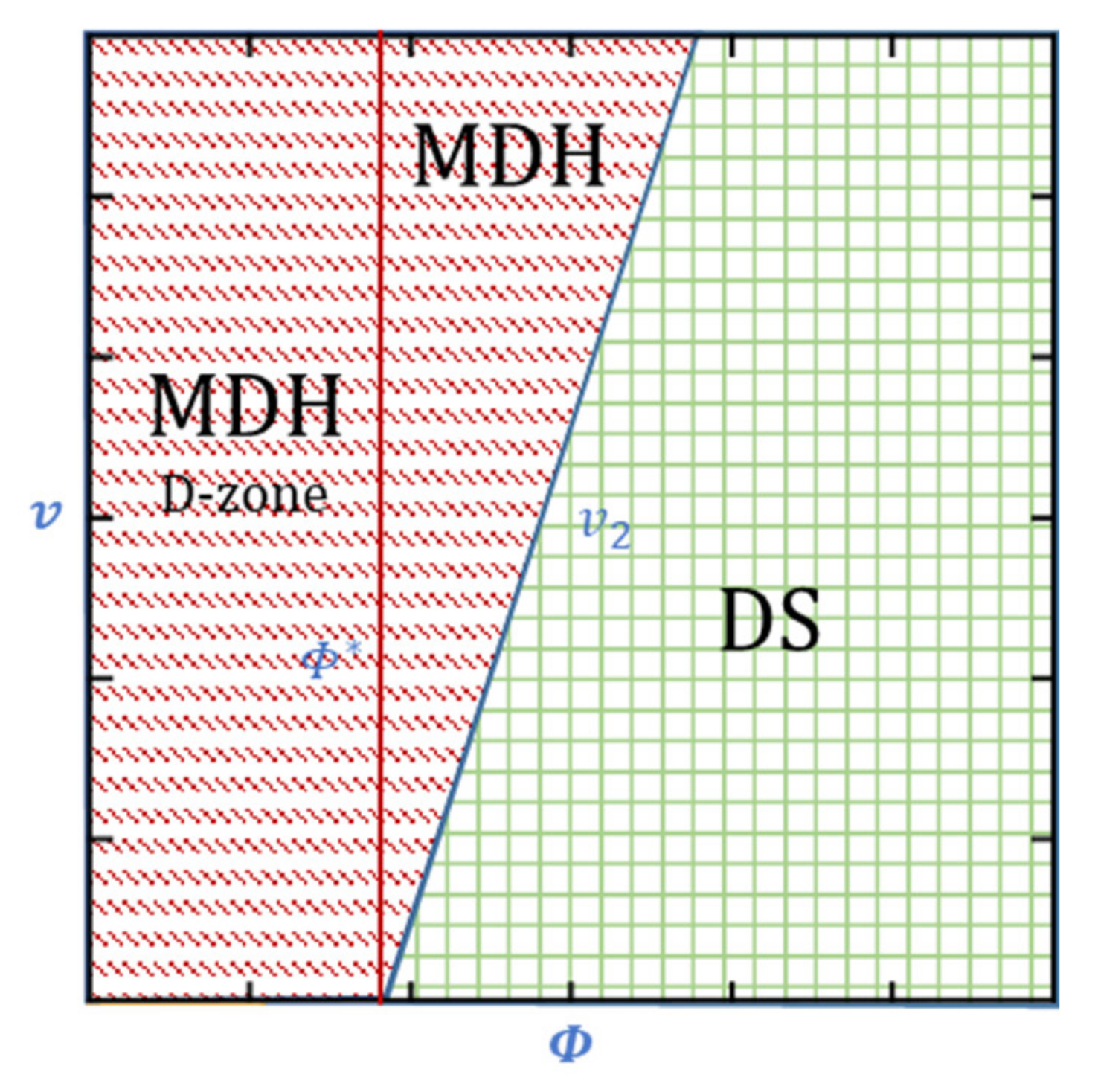
For the comparison between MDH and DS strategies, we found that when IoT operation cost is low ($\Phi \left({\tau }_H\right)<X_2$), the MDH strategy dominates the DS strategy at any condition, which is intuitive because implementing MDH would not incur large costs as upgrading the tracking system is less costly. When we further analyze the structure of $X_2$, we found that the tradeoff of choosing MDH or DS is twofold. One is whether the cost of upgrading the system can be mitigated by gaining from traceability improvement. The saving in communication costs is the main source of potential gain. The other is that a high natural failure rate ($P^L$) will incentive the company to choose the MDH strategy. Specifically, if TNS customers also value basic traceability, then the burden for the company to implement the MDH will also ease. As shown in Figure 7, we indicate the MDH domination zone where $\Phi \left({\tau }_H\right)$ is low. However, if the $\Phi \left({\tau }_H\right)$ is at the intermediate level, then MDH is only better-off when $v$ is high. The reason is that as the freight value $v$ increases, reducing the overall failure rate and avoiding failure in the TNS segment will be more meaningful.

As we know, HT and MDH strategies have public interest attributes, and the company either charges no additional fee on TNS customers (MDH) or charges a relatively low price (HT) when supplying both segments with high-traceability service. When a company wants to maximize its profit (under MDH and HT), we would like to explore whether the strategies maximize social welfare (compared with other strategies). We will focus on deriving the market conditions for the HT/MDH to maximize social welfare when the company implements its profit-maximization pricing decision.

4.3. Social Welfare Analysis

Social welfare in this study is defined as the sum of the company’s profit and customers’ utility. We denote ${\pi }_{\left(A,B\right)}^{SOC}$ as the social welfare under each strategy, where $Aϵ\left\{L,H,LH,\varphi \right\}, Bϵ\left\{L,H\right\}$.

Table 4. Social Welfare Difference.

	HT	MDH
DS	$n_{TNS}\left({\Delta }_{TNS}+\left(P^L-P^H\right)v+P^{L}C-\Phi \left({\tau }_H\right)\right)$	$n_{TNS}\left(\lambda \mathrm{r}\left(P^L-P^H\right)+P^{L}C-\Phi \left({\tau }_H\right)\right)$
HES	$n_{TNS}\left(\left(1-P^H\right)v+{\alpha }_{TNS}\left({\tau }_H\right)-\Phi \left({\tau }_H\right)\right)$	$n_{TNS}\left(\left(1-P^L\right)v+{\alpha }_{TNS}\left({\tau }_0\right)+\lambda \mathrm{r}\left(P^L-P^H\right)-\Phi \left({\tau }_H\right)\right)$
LT	$\left(P^L-P^H\right)v+n_{TS}{\Delta }_{TS}+n_{TNS}{\Delta }_{TNS}+P^{L}C-\Phi \left({\tau }_H\right)$	$\left(n_{TS}v+n_{TNS}\lambda \mathrm{r}\right)\left(P^L-P^H\right)+n_{TS}{\Delta }_{TS}+P^{L}C-\Phi \left({\tau }_H\right)$

shows the social welfare difference between HT/MDH and other strategies:

Note $r=r_{MDH}^{*}=\frac{\left(1-P^L\right)v+{\alpha }_{TNS}\left({\tau }_0\right)}{1-\lambda P^L}$. The difference between MDH and HT strategy is ${\pi }_{\left(H,H\right)}^{SOC}-{\pi }_{\left(LH,H\right)}^{SOC}=n_{TNS}\left[{\Delta }_{TNS}-\left(P^L-P^H\right)\left(\lambda \mathrm{r}-v\right)\right]$, where $r=r_{MDH}^{*}$.

We then derive the following findings:

Remark 1.

Whether the HT/MDH strategy outperforms other strategies on social welfare maximization depends on two issues. One question to ask is “is it worth to invest in reducing the delivery failure rate”? HT/MDH is a costly IoT adoption strategy, and both strategies require a complete upgrade of the delivery system. From the comparison between HT/MDH and DS/HES/LT strategies, we found the consequence of delivery failure gets severe when the freight value increases. Then, HT/MDH strategies show an advantage in reducing the waste of social productive forces. However, when the IoT operation cost is high, the goodwill of HT/MDH to reduce delivery failure shifts to negative effects and the high-traceability system also becomes a waste of resources. The other question to ask is, “how much do the TNS customers value the real-time logistics information”? The MDH blocks real-time logistics information to TNS customers and neglects TNS customers’ valuation on traceability improvement. When we compare the social welfare of HT and MDH strategies, if TNS customers’ valuation is also considerable, then directly providing high traceability to both segments will be beneficial to social welfare. Combined with the findings in Proposition 8, the company’s profit will also improve. Therefore, market investigation on customers segments is crucial.

Proof. 

Please refer to Appendix A for the derivative process. □

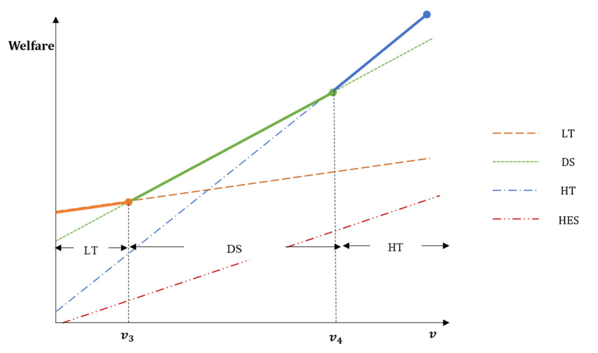
Figure 8 shows that as $v$ increases, the social welfare optimizing strategy switches from LT → DS → HT/MDH, which means that completely upgrading the delivery system (from the social welfare aspect) is noteworthy only when the freight value is high. We omit the MDH in Figure 8 because it is similar to the line of HT.

5. Insights and Conclusions

With booming e-commerce around the world, the safety and security issues of e-commerce logistics have become more significant. The failures in e-commerce delivery significantly affect customers’ welfare and waste social resources. Given the industry practice of the leading E-retailer, JD has included high-traceability logistics service (based on IoT technology) as a value-added service in their business model, the present study builds analytical models to investigate the effect of E-retailer’s IoT adoption decisions on the social welfare and firm’s profitability. The main contributions of our paper and comparisons to some earlier key studies are summarized as follows.

As Panova et al. [57] pointed out, e-retailers pay attention to delivery quality control issues in order to enhance the successful transaction rate. Our study confirms that the adoption of the IoT-based tracking system in e-commerce logistics operations can significantly improve delivery quality and reduce the failure rate.

We studied the E-retailer’s compensation policy for delivery failure, pricing decision of delivery service, and optimal IoT adoption decision. We found that E-retailers have full incentive to reduce delivery failure, as the delivery quality is their core competitiveness. This finding is consistent with Zheng et al. [58]. Setting a high compensation rate for delivery failure can enhance the profitability of the E-retailer when delivery quality is high. However, when delivery quality is poor, it can significantly hurt the E-retailer’s profitability, so relying on compensation policy cannot save the company from loss. At the same time, the customers value logistics traceability more, and in particular, the customers who purchase high-value products care more about delivery quality. These study results support the findings of Cui et al. [59]. We analyzed the optimal pricing decision of each IoT adoption strategy and illustrated how an IoT adoption strategy can contribute to the E-retailer’s profit and social welfare. The company’s IoT operation cost and problem-resolving cost will affect the selection of optimal IoT strategy.

Some of our findings can be further refined to the following guidelines for managers in E-retailer with its self-built logistics arm (e.g., JD and Amazon, SF Express) to apply appropriate IoT adoption strategies in different market conditions.

First, the E-retailer should sufficiently make use of accumulated consumer big data and depict a customer valuation model on traceability. We show that the power of full information advantage can significantly strengthen the performance of IoT adoption, specifically, acquiring full information of customers will enhance the profitability when E-retailer implements a differentiated service strategy. Necessary information to depict a customer valuation model, such as the consumption habit for each particular consumer, can be retrieved from the cloud and should be effectively extracted for the mining of essential knowledge to facilitate decision making. An E-retailer, especially for an industry leader, such as JD, might readily have such data at its disposal. More detailed discussion of analyzing consumer big data has been addressed by the academic community [60].

Second, the decision-makers shall be careful with the trap of “conservative strategy”. We illustrate that the optimal IoT adoption changes under different market conditions, thus implementing a comprehensive investigation (on the company’s internal operations efficiency, customers’ properties) is required before adopting a specific strategy. When comprehensive market research is not available, adopting a conservative strategy is intuitive for decision-makers, for example, launching high-traceability services in certain market segments while maintaining the basic services in the remaining market (which is the DS strategy in our context). However, such a conservative strategy could lead to suboptimum results. For example, we conclude E-retailer always completely adopts IoT technology in both segments when the adoption cost is low (HT strategy) and not adopted when the cost is sufficiently high. As the IoT adoption cost increases, and optimal strategy switches from HT to LT. Such a finding is intuitive. However, the DS strategy does not necessarily appear as an optimal strategy that provides the highest profitability when the IoT adoption cost is at the intermediate level. When the problem-resolving cost of E-retailer is high and IoT adoption cost at intermediate level, the HES strategy (exit TNS customer segment and only serve TS segment with high-traceability service) could be the optimal strategy. Such a counterintuitive strategy is not easy to find and implement without a comprehensive understanding of the market and the company’s internal operation situation. Adopting HES as optimal strategy is realistic—for an E-retailer with a good reputation, for example, JD and Vipshop—the customers prefer to purchase the specific type of product from the website since trust their service quality. When the customers complain on social media about a delivery failure, it will hurt the image of the company and threaten their industry leadership, which causes high problem-resolving costs. Thus, the company prefers to only serve the TS customer with high-traceability service to avoid service failure.

Third, IoT adoption is not necessarily beneficial to both social welfare and E-retailer’s profitability under certain circumstances. Currently, the market has many available IoT-based tracking system solution providers. The E-retailer could choose whether to purchase from these providers (for example, Hanhaa) or to develop a tracking system by themselves (as JD). As we show in the analysis part, the company shall not adopt IoT either when adoption cost is high (adoption hurts the profit of E-retailer) or when the freight value is not high enough (adoption hurts the social welfare). When E-retailer implements HT strategy or MDH strategy, its behavior objectively participates in corporate social responsibility (the subjective intention is maximizing profit). However, an exorbitant IoT operations cost might cause a waste of social resources. If the company decides to develop by themselves, then it should focus on the durability of their IoT equipment. The short-life IoT hardware will deepen the social resource waste. If the company chooses to procure, they shall make use of their bargaining power to acquire cost-effective IoT solutions to enhance social welfare. When acquiring the IoT solutions at a low rate is not applicable, promoting the internal operational efficiency of the company to reduce the company’s problem-resolving cost, and choosing not to adopt IoT will enhance profitability and maximize social welfare. These findings are somewhat similar to Yu et al. [61]. They illustrate, even if launching IoT devices to collect data in E-commerce logistics and thus deriving rich knowledge to support decision-makings are indeed attractive, the company shall always balance their service and corresponding cost.

We recognize that our models have limitations. Our analysis was conducted in the absence of competition. We expect the presence of competition to further increase the environmental impact as the company’s pricing decision will be affected if the competitor enters in same customer segments. However, the presence of competition might also improve overall social welfare. We adopt the implicit function format for customer valuations on traceability and the company’s IoT operation cost as we not yet find solid empirical results in the literature. Therefore, the research that adopts an explicit utility function will provide inspired insights. Similarly, research about the company’s IoT adoption strategies in the multi-period competition is also an exciting direction for future research because we omitted the impact of the scale effect when the company invests in IoT technology.

References

1. State Post Bureau of the People’s Republic of China. China Express Development Index Report-2020. Available online: http://www.spb.gov.cn/xw/dtxx_15079/202105/t20210508_3898077.html (accessed on 1 July 2021). (In Chinese)
2. UN News. Global E-Commerce Jumps to $26.7 Trillion, Fuelled by COVID-19. Available online: https://news.un.org/en/story/2021/05/1091182 (accessed on 2 July 2021).
3. World Economic Forum. The Future of the Last-Mile Ecosystem. Available online: http://www3.weforum.org/docs/WEF_Future_of_the_last_mile_ecosystem.pdf (accessed on 1 July 2021).
4. Delivered. Wrap Battle: How to Tackle E-Commerce Packaging Waste. Available online: https://www.dhl.com/global-en/home/about-us/delivered-magazine/articles/2019/issue-2-2019/tackle-ecommerce-packaging-waste.html (accessed on 1 July 2021).
5. Dropoff. Consumers Want Faster Delivery and They’re Willing to Pay for It. Available online: https://www.dropoff.com/blog/retail-delivery-consumer-survey-shoptalk-2018/ (accessed on 1 July 2021).
6. State Post Bureau of the People’s Republic of China. Notice of the State Post Bureau on September 2019 Consumer Complaints in the Postal Industry. Available online: http://www.gov.cn/xinwen/2019-10/23/content_5443946.htm (accessed on 1 July 2021). (In Chinese)
7. Tian, Z.; Zhong, R.Y.; Vatankhah Barenji, A.; Wang, Y.; Li, Z.; Rong, Y. A blockchain-based evaluation approach for customer delivery satisfaction in sustainable urban logistics. Int. J. Prod. Res. 2021, 59, 2229–2249. [Google Scholar] [CrossRef]
8. Citizens Advice. Citizens Advice Says Problems with Parcels Cost Consumers at least £85 Million a Year. Available online: https://www.citizensadvice.org.uk/about-us/about-us1/media/press-releases/citizens-advice-says-problems-with-parcels-cost-consumers-at-least-85-million-a-year/ (accessed on 1 July 2021).
9. Reltronics Technologies. Cargo & Shipment Tracking. Available online: http://reltronicstech.com/Cargo_Shipment_Tracking.html (accessed on 4 July 2021).
10. Valley Box Company. RFID in the Packaging and Shipping Industry. Available online: https://www.valleybox.com/blog/rfid-in-the-packaging-and-shipping-industry (accessed on 4 July 2021).
11. Tweak Your Biz. Reduce Shipping Damage and Delays with RFID Tracking. Available online: https://tweakyourbiz.com/business/rfid-package-tracking (accessed on 4 July 2021).
12. Bonnington, C. Here’s How to Track Your Amazon Packages in Real Time. The Daily Dot. Available online: https://www.dailydot.com/debug/amazon-map-tracking/ (accessed on 6 July 2021).
13. Hanhaa. Shareable Link: Instantly View A Customer Journey on the ParceLive Portal! Available online: https://hanhaa.com/shareable-link-instantly-view-a-customer-journey-on-the-parcelive-portal/ (accessed on 4 July 2021).
14. Benton, D. ParceLive: IoT and Real-Time Parcel Tracking Technology. Available online: https://supplychaindigital.com/logistics-1/parcelive-iot-and-real-time-parcel-tracking-technology (accessed on 1 July 2021).
15. Dickey, C. Demystifying “Track & Trace” vs “Real-Time Tracking” vs “Monitoring”. Available online: https://blog.roambee.com/supply-chain-technology/demystifying-track-trace-vs-real-time-tracking-vs-monitoring (accessed on 2 July 2021).
16. Arviem. Real-Time Cargo and Container Monitoring. Available online: https://arviem.com/track-and-trace-container-tracking/ (accessed on 2 July 2021).
17. Sun, Y. Twenty Times in Ten Years, American LTL Giant ODFL In-Depth Review. Available online: https://mp.weixin.qq.com/s/aHcMw-dVipkk2B51u_-RTA (accessed on 1 July 2021). (In Chinese).
18. YTO Express 2019 Annual Report. Available online: https://mp.weixin.qq.com/s/jgXO90RL9HDzD-Kpm8UIHA (accessed on 24 May 2021). (In Chinese).
19. Zhang, Y.; Liu, S.; Liu, Y.; Li, R. Smart box-enabled product–service system for cloud logistics. Int. J. Prod. Res. 2016, 54, 6693–6706. [Google Scholar] [CrossRef]
20. Sui, X. JD Express Launches New Service “Feather Letter”: Real-Time Tracking of Parcels. Available online: https://news.mydrivers.com/1/625/625893.html (accessed on 2 July 2021). (In Chinese).
21. Ramanathan, R. The moderating roles of risk and efficiency on the relationship between logistics performance and customer loyalty in e-commerce. Transp. Res. E Logist. Transp. Rev. 2010, 46, 950–962. [Google Scholar] [CrossRef]
22. Bowersox, D.J.; Closs, D.J.; Cooper, M.B. Supply Chain Logistics Management, 3rd ed.; The McGraw-Hill/Irwin Series Operations and Decision Sciences: Boston, MA, USA, 2010; p. 65. [Google Scholar]
23. Mentzer, J.T.; Rutner, S.M.; Matsuno, K. Application of the means-end value hierarchy model to understanding logistics service value. Int. J. Phys. Distrib. Logist. Manag. 1997. [Google Scholar] [CrossRef]
24. Zhao, H. How Do Express Companies Get Away with Anxiety? Available online: https://mp.weixin.qq.com/s/Odws0j53VuqGEvvtoB7HvQ (accessed on 13 May 2021). (In Chinese).
25. Welch, C. UPS Now Lets You Track Packages for Real—On an Actual Map. Available online: https://www.theverge.com/2016/5/12/11668602/ups-follow-my-delivery-map-tracking-now-available (accessed on 1 July 2021).
26. Clark, E. Package Theft Statistics: People Trust UPS the Most to Deliver Packages Safely. Available online: https://clutch.co/report/package-theft-statistics-people-trust-ups-most-deliver-packages-safely (accessed on 2 July 2021).
27. Chen, Q.; Zhou, H.; Zhang, D.; Xiao, X. “Post 90s” Express Life Report. Available online: https://mp.weixin.qq.com/s/pWwzDgyDXjDqkTiirltvng (accessed on 6 July 2021).
28. Balakrishnan, A.; Natarajan, H.P. Designing fee tables for retail delivery services by third-party logistics providers. IIE Trans. 2014, 46, 1261–1278. [Google Scholar] [CrossRef] [Green Version]
29. Zikopoulos, C. Determination of freight rates under stochastic demand and freight consolidation savings. Int. J. Prod. Res. 2019, 57, 5556–5573. [Google Scholar] [CrossRef]
30. Wu, Q.; Mu, Y.; Feng, Y. Coordinating contracts for fresh product outsourcing logistics channels with power structures. Int. J. Prod. Econ. 2015, 160, 94–105. [Google Scholar] [CrossRef]
31. Yu, Y.; Xiao, T. Pricing and cold-chain service level decisions in a fresh agri-products supply chain with logistics outsourcing. Comput. Ind. Eng. 2017, 111, 56–66. [Google Scholar] [CrossRef]
32. Wang, Y.-Y.; Li, J. Research on pricing, service and logistic decision-making of E-supply chain with ‘Free Shipping’ strategy. J. Control. Decis. 2018, 5, 319–337. [Google Scholar] [CrossRef]
33. Lukassen, P.J.; Wallenburg, C.M. Pricing third-party logistics services: Integrating insights from the logistics and industrial services literature. Transp. J. 2010, 49, 24–43. [Google Scholar]
34. Liu, W.; Yan, X.; Wei, W.; Xie, D. Pricing decisions for service platform with provider’s threshold participating quantity, value-added service and matching ability. Transp. Res. E Logist. Transp. Rev. 2019, 122, 410–432. [Google Scholar] [CrossRef]
35. Dai, H.; Tseng, M.M.; Zipkin, P.H. Design of traceability systems for product recall. Int. J. Prod. Res. 2015, 53, 511–531. [Google Scholar] [CrossRef]
36. Hobbs, J.E. Information asymmetry and the role of traceability systems. Agribus. Int. J. 2004, 20, 397–415. [Google Scholar] [CrossRef]
37. Aung, M.M.; Chang, Y.S. Traceability in a food supply chain: Safety and quality perspectives. Food Control 2014, 39, 172–184. [Google Scholar] [CrossRef]
38. Resende-Filho, M.A.; Hurley, T.M. Information asymmetry and traceability incentives for food safety. Int. J. Prod. Econ. 2012, 139, 596–603. [Google Scholar] [CrossRef]
39. Starbird, S.A.; Amanor-Boadu, V. Traceability, inspection, and food safety. In Proceedings of the Agricultural and Applied Economics Association (AAEA) 2004 Annual Meeting (No. 377-2016-20880), Denver, CO, USA, 1–4 August 2004. [Google Scholar]
40. Sun, S.; Wang, X. Promoting traceability for food supply chain with certification. J. Clean. Prod. 2019, 217, 658–665. [Google Scholar] [CrossRef]
41. Wang, X.; Li, D.; Li, L. Adding value of food traceability to the business: A supply chain management approach. Int. J. Serv. Oper. Inform. 2009, 4, 232–257. [Google Scholar] [CrossRef]
42. Wang, X.; Li, D.; O’brien, C.; Li, Y. A production planning model to reduce risk and improve operations management. Int. J. Prod. Econ. 2010, 124, 463–474. [Google Scholar] [CrossRef]
43. De Vass, T.; Shee, H.; Miah, S.J. The effect of “Internet of Things” on supply chain integration and performance: An organisational capability perspective. Australas. J. Inf. Syst. 2018, 22. [Google Scholar] [CrossRef] [Green Version]
44. De Vass, T.; Shee, H.; Miah, S.J. Iot in supply chain management: A narrative on retail sector sustainability. Int. J. Logist. Res. Appl. 2020, 1–20. [Google Scholar] [CrossRef]
45. Rekik, Y.; Syntetos, A.A.; Glock, C.H. Modeling (and Learning from) Inventory Inaccuracies in E-retailing/B2B contexts. Decis. Sci. 2019, 50, 1184–1223. [Google Scholar] [CrossRef]
46. Fan, T.-J.; Chang, X.-Y.; Gu, C.-H.; Yi, J.-J.; Deng, S. Benefits of RFID technology for reducing inventory shrinkage. Int. J. Prod. Econ. 2014, 147, 659–665. [Google Scholar] [CrossRef]
47. Zhang, L.-H.; Li, T.; Fan, T.-J. Radio-frequency identification (RFID) adoption with inventory misplacement under retail competition. Eur. J. Oper. Res. 2018, 270, 1028–1043. [Google Scholar] [CrossRef]
48. Tao, F.; Fan, T.; Lai, K.K.; Li, L. Impact of RFID technology on inventory control policy. J. Oper. Res. Soc. 2017, 68, 207–220. [Google Scholar] [CrossRef]
49. Fan, T.; Tao, F.; Deng, S.; Li, S. Impact of RFID technology on supply chain decisions with inventory inaccuracies. Int. J. Prod. Econ. 2015, 159, 117–125. [Google Scholar] [CrossRef]
50. Biswal, A.K.; Jenamani, M.; Kumar, S.K. Warehouse efficiency improvement using RFID in a humanitarian supply chain: Implications for Indian food security system. Transp. Res. E Logist. Transp. Rev. 2018, 109, 205–224. [Google Scholar] [CrossRef]
51. Qin, W.; Zhong, R.Y.; Dai, H.; Zhuang, Z. An assessment model for RFID impacts on prevention and visibility of inventory inaccuracy presence. Adv. Eng. Inform. 2017, 34, 70–79. [Google Scholar] [CrossRef]
52. Chadha, S.S.; Ülkü, M.A.; Venkatadri, U. Freight delivery in a Physical Internet Supply Chain: An applied optimisation model with peddling and shipment consolidation. Int. J. Prod. Res. 2021, 1–17. [Google Scholar] [CrossRef]
53. Ben-Daya, M.; Hassini, E.; Bahroun, Z. Internet of things and supply chain management: A literature review. Int. J. Prod. Res. 2019, 57, 4719–4742. [Google Scholar] [CrossRef] [Green Version]
54. Erkut, E.; Verter, V. Modeling of transport risk for hazardous materials. Oper. Res. 1998, 46, 625–642. [Google Scholar] [CrossRef] [Green Version]
55. Package Guard. Amazon A-to-Z Guarantee Lost & Stolen Package Fact Sheet. Available online: https://thepackageguard.com/package-theft/amazon-package-theft/ (accessed on 2 July 2021).
56. Package Guard. Package Guard Guide to a Missing UPS Package. Available online: https://thepackageguard.com/package-theft/ups-package-theft/ (accessed on 2 July 2021).
57. Panova, Y.; Tan, A.; Hilmola, O.-P.; Puvindran, M.; Hongsheng, X.; Li, W. Evaluation of e-commerce location and entry to China–implications on shipping and trade. J. Ship. Trade 2019, 4, 1–25. [Google Scholar] [CrossRef]
58. Zheng, K.; Zhang, Z.; Song, B. E-commerce logistics distribution mode in big-data context: A case analysis of JD. COM. Ind. Mark. Manag. 2020, 86, 154–162. [Google Scholar] [CrossRef]
59. Cui, R.; Li, M.; Li, Q. Value of high-quality logistics: Evidence from a clash between SF Express and Alibaba. Manag. Sci. 2020, 66, 3879–3902. [Google Scholar] [CrossRef]
60. Zhao, Y.; Zhou, Y.; Deng, W. Innovation mode and optimization strategy of B2C e-commerce logistics distribution under big data. Sustainability 2020, 12, 3381. [Google Scholar] [CrossRef] [Green Version]
61. Yu, Y.; Wang, X.; Zhong, R.Y.; Huang, G.Q. E-commerce logistics in supply chain management: Implementations and future perspective in furniture industry. Ind. Manag. Data Syst. 2017, 117, 2263–2286. [Google Scholar] [CrossRef]
Figure 1. Fragmented logistics information on JD.
Sustainability 13 10597 g001
Figure 2. Traceability system based on smart pallet.
Sustainability 13 10597 g002
Figure 3. Delivery failure rate calculation.
Sustainability 13 10597 g003
Figure 4. Optimal Strategy Region Changes as TS Segment Expands.
Sustainability 13 10597 g004
Figure 5. Optimal Strategy Region Changes as FB-DS Introduced. (1) DS under Information Asymmetric; (2) DS under Full Information.
Sustainability 13 10597 g005
Figure 6. Optimal Strategy Region Changes as TS Segment Expands (MDH vs. HT, v 1 = X 1 n T S Δ T S Y 1 , Δ T S * = X 1 n T S ). (1) Small TS segment; (2) Large TS segment.
Sustainability 13 10597 g006
Figure 7. Optimal Strategy Region (MDH vs. DS) ( v 2 = Φ τ H X 2 Y 2 , Φ * = X 2 ).
Sustainability 13 10597 g007
Figure 8. Social Welfare Maximizing Strategy as Freight Value Increases.
Sustainability 13 10597 g008