
Prediction of Aquatic Ecosystem Health Indices through Machine Learning Models Using the WGAN-Based Data Augmentation Method


Abstract
1. Introduction
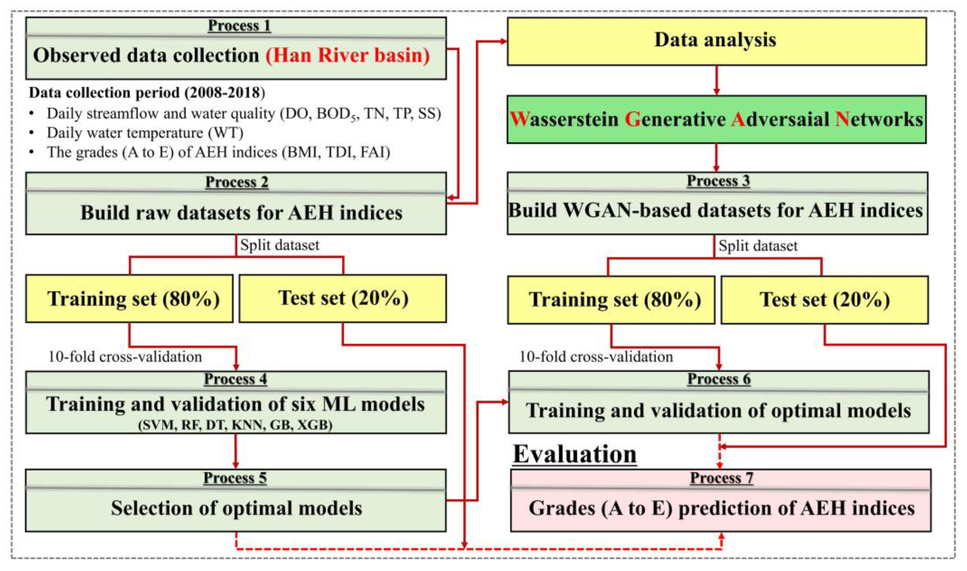
2. Materials and Methods
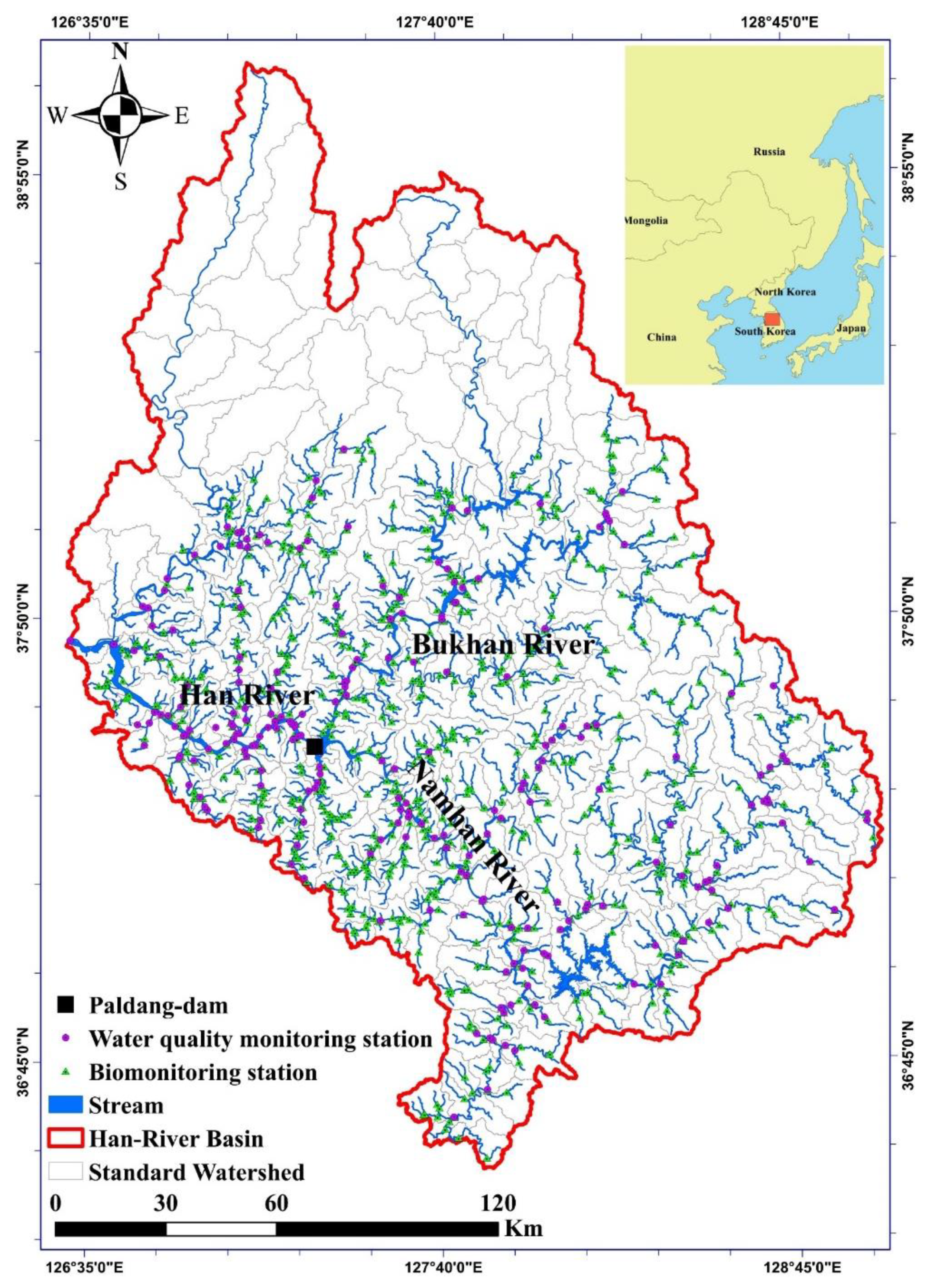
2.1. Description of the Study Area
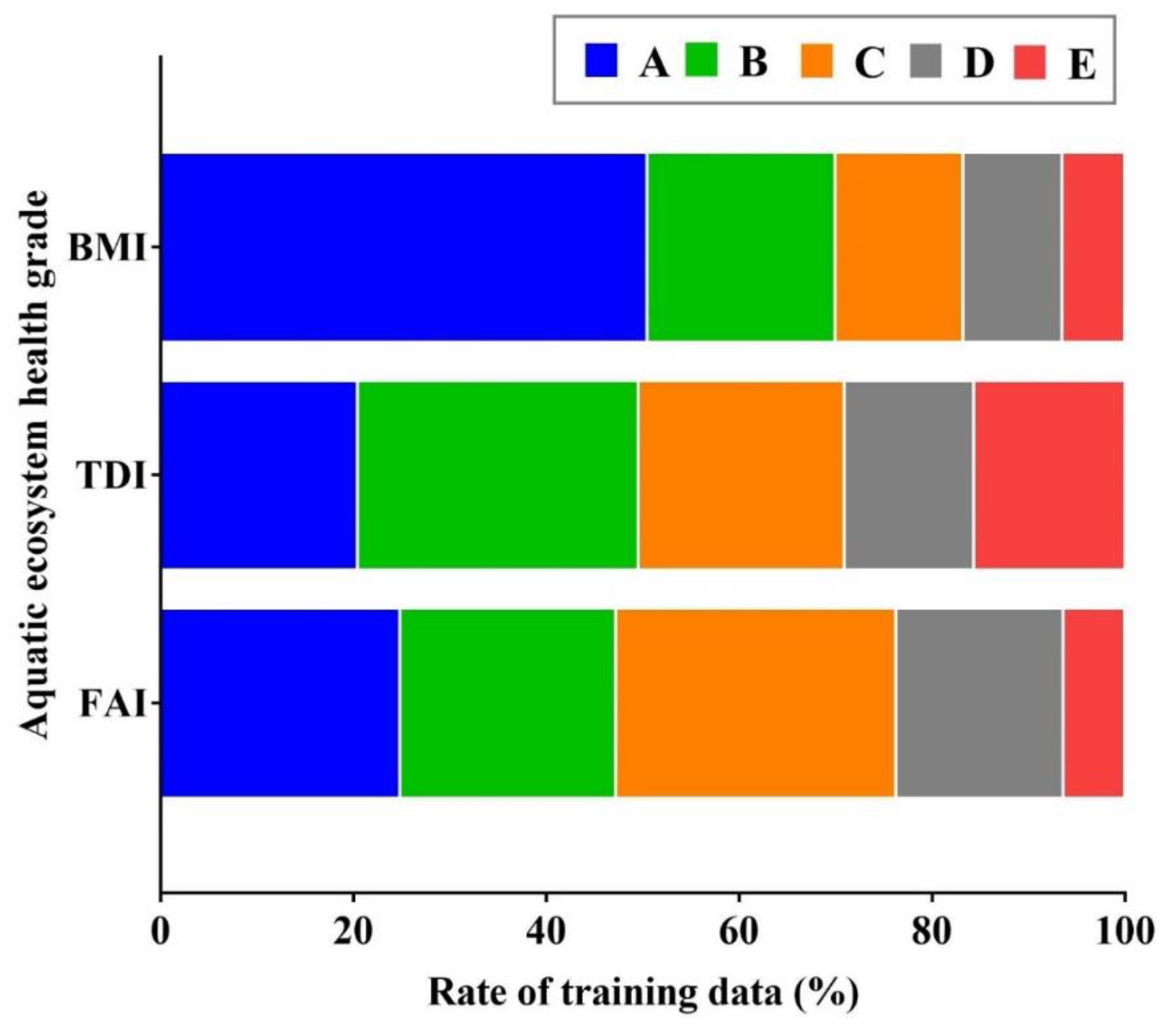
2.2. Data Collection
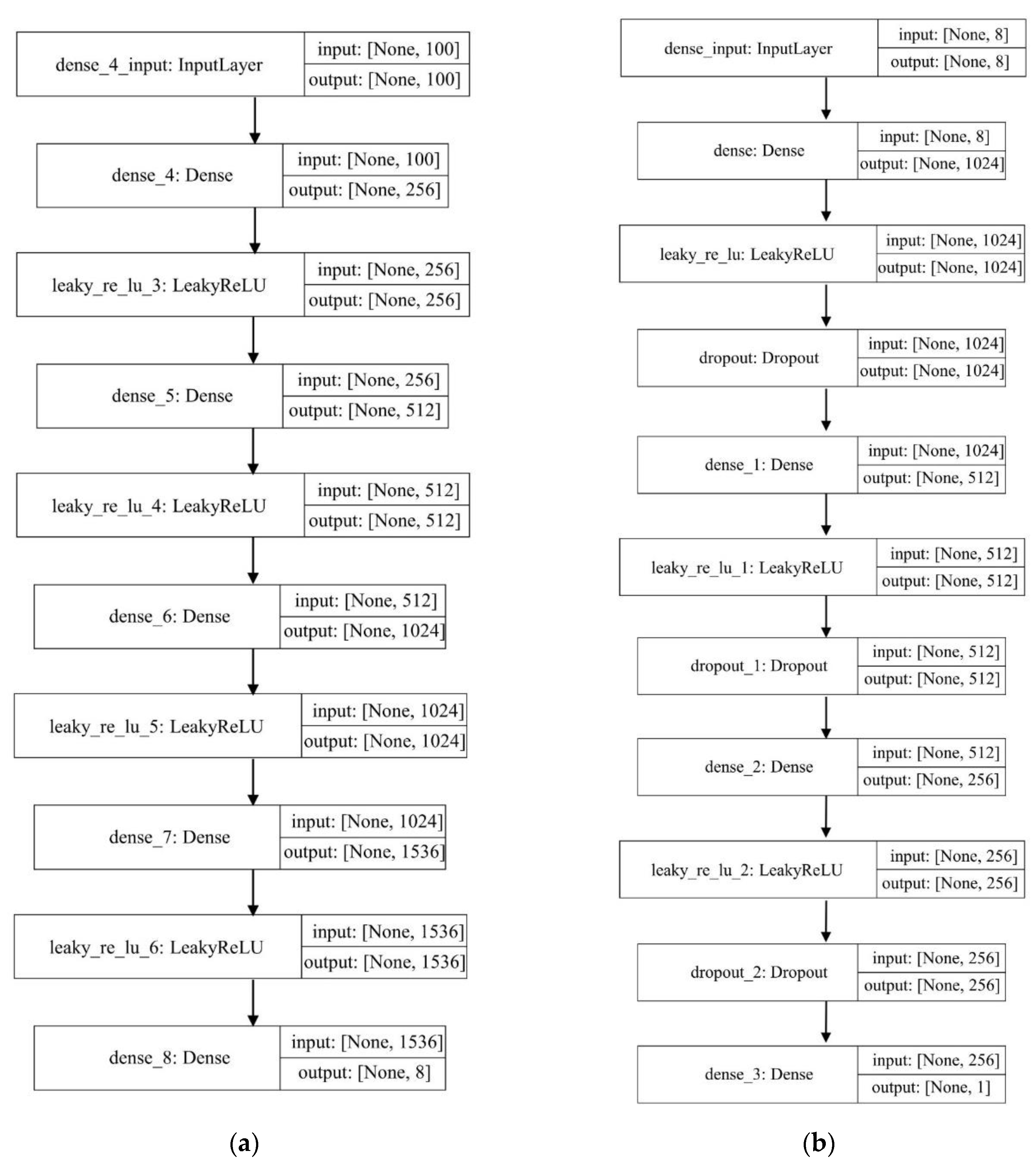
2.3. Wasserstein Generative Adversarial Network (WGAN)
2.4. Building and Evaluation of ML Models
2.4.1. ML Models Building and Evaluation Process
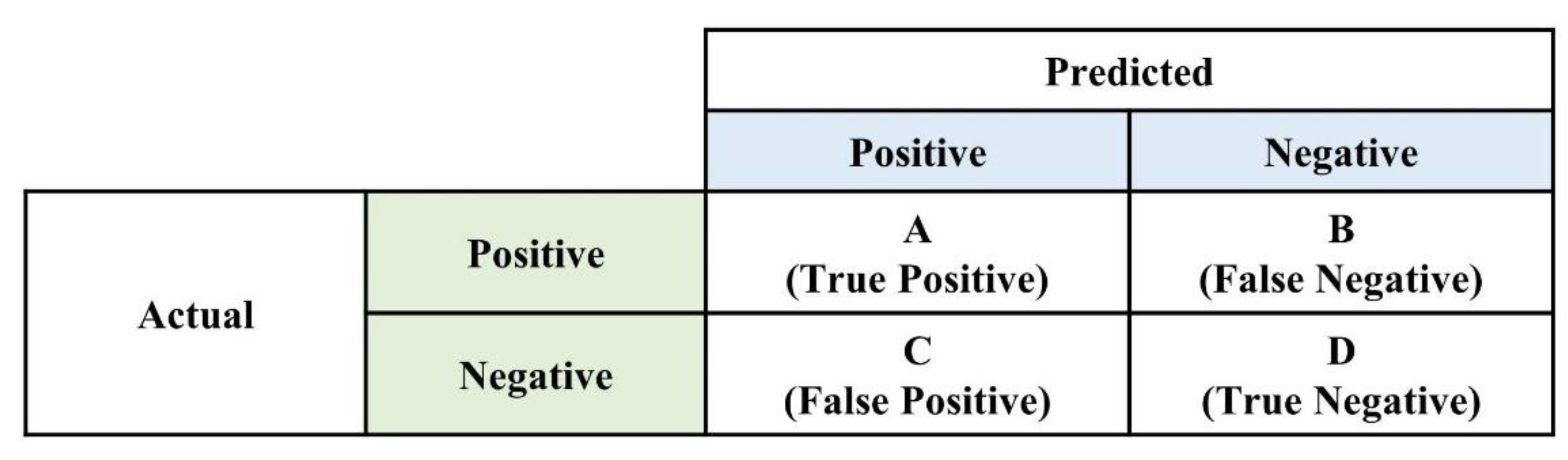
2.4.2. The Performance Evaluation Metrics of ML Models
3. Results and Discussion
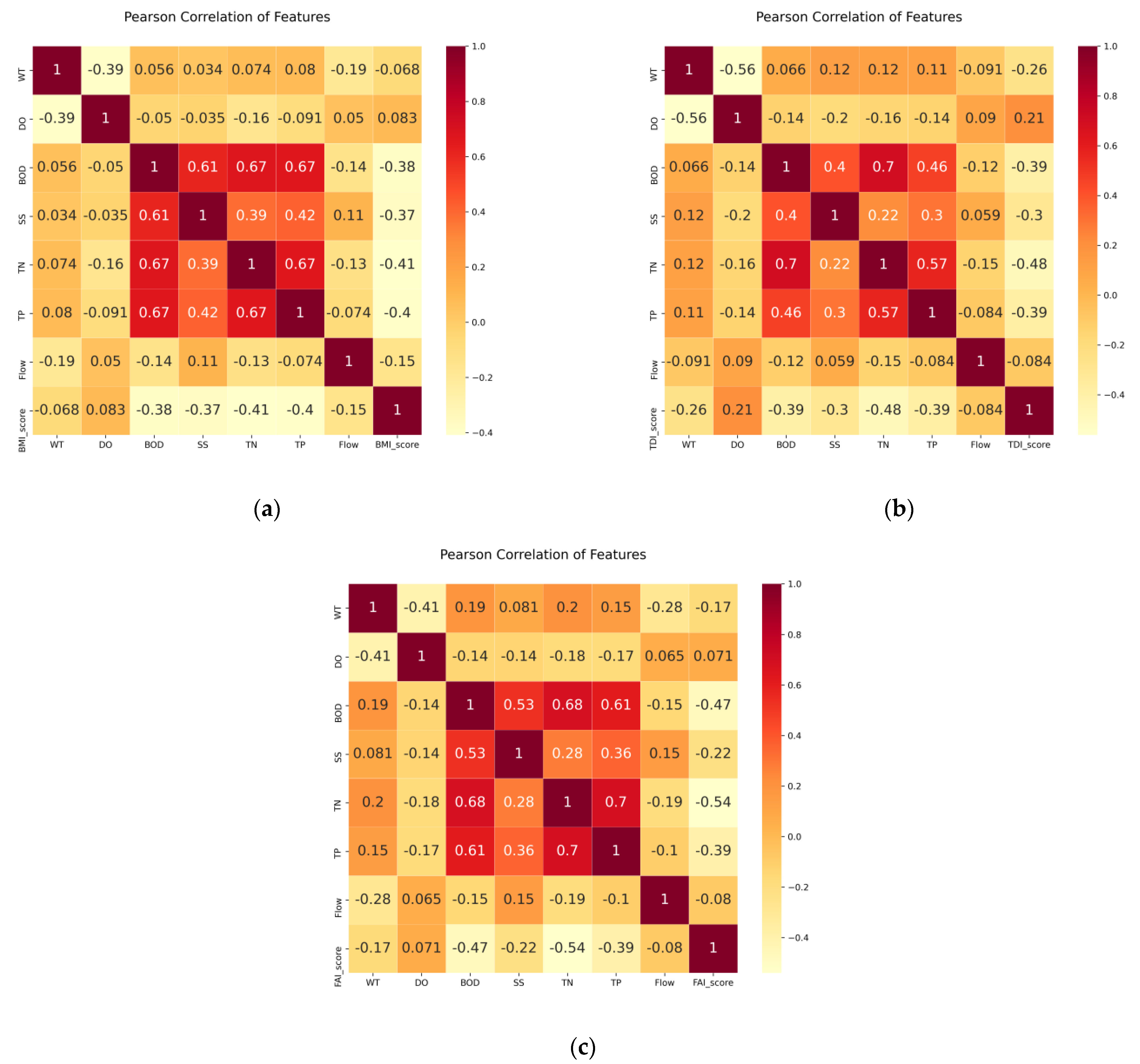
3.1. Correlation Analysis Results
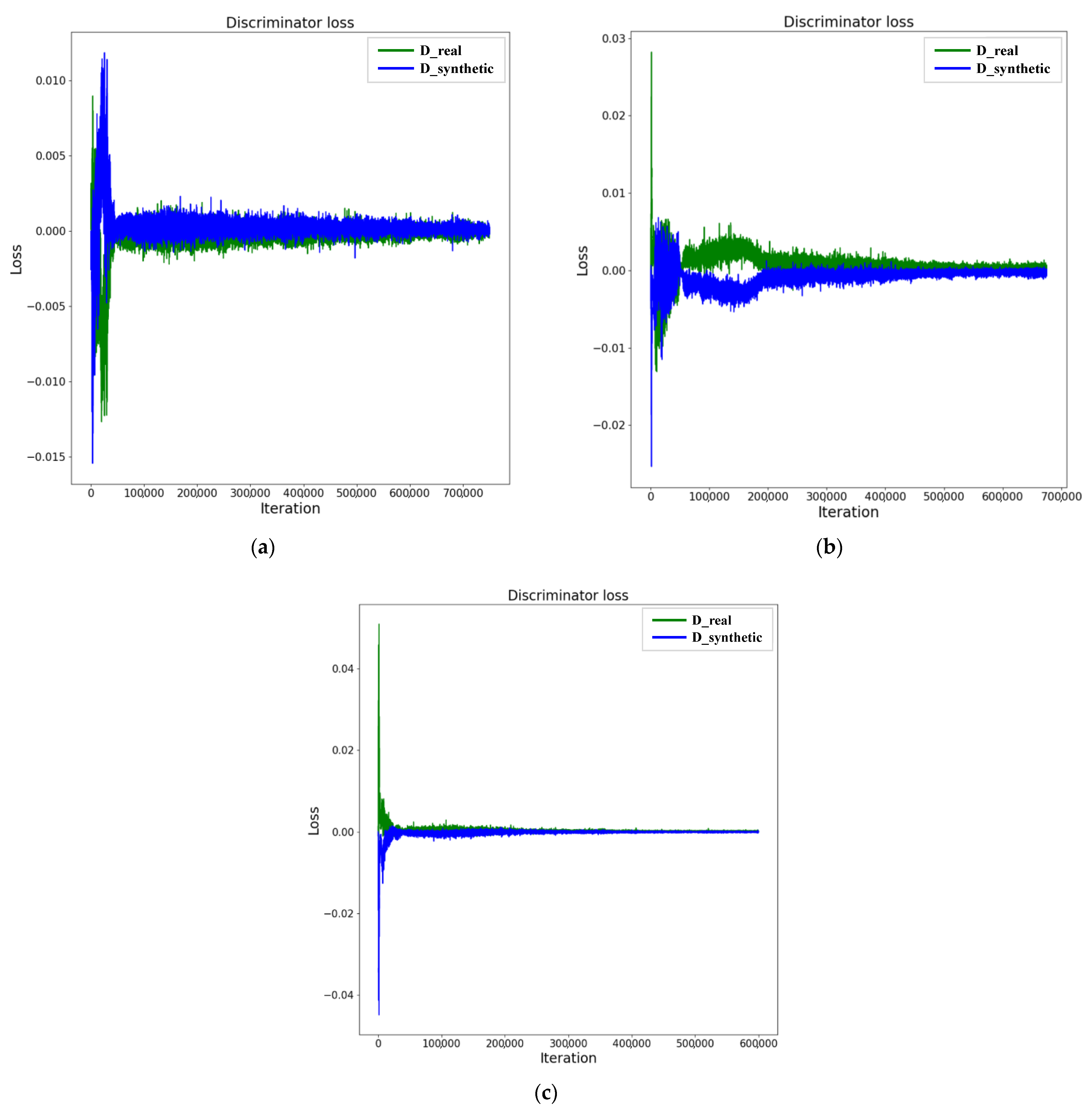
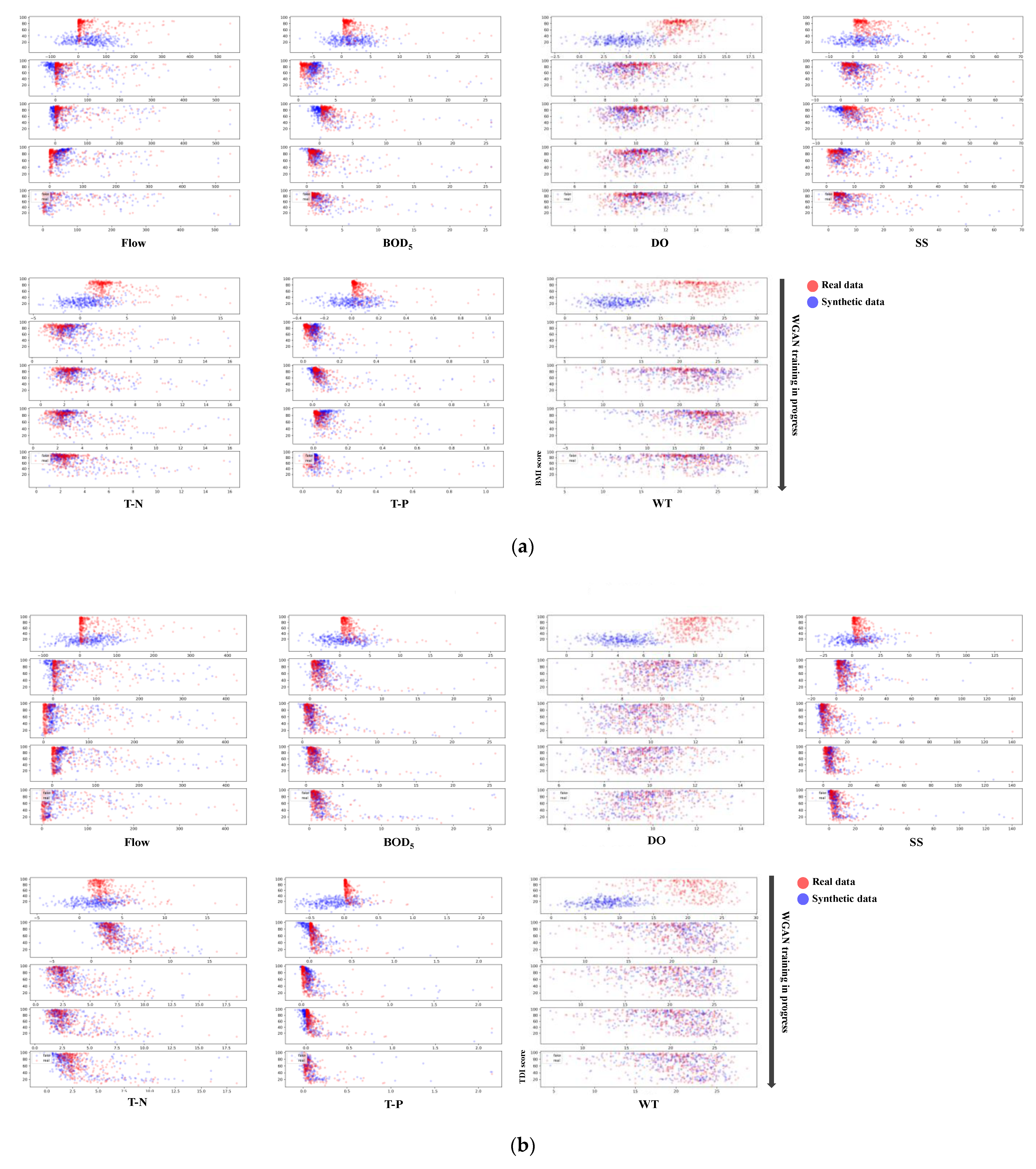
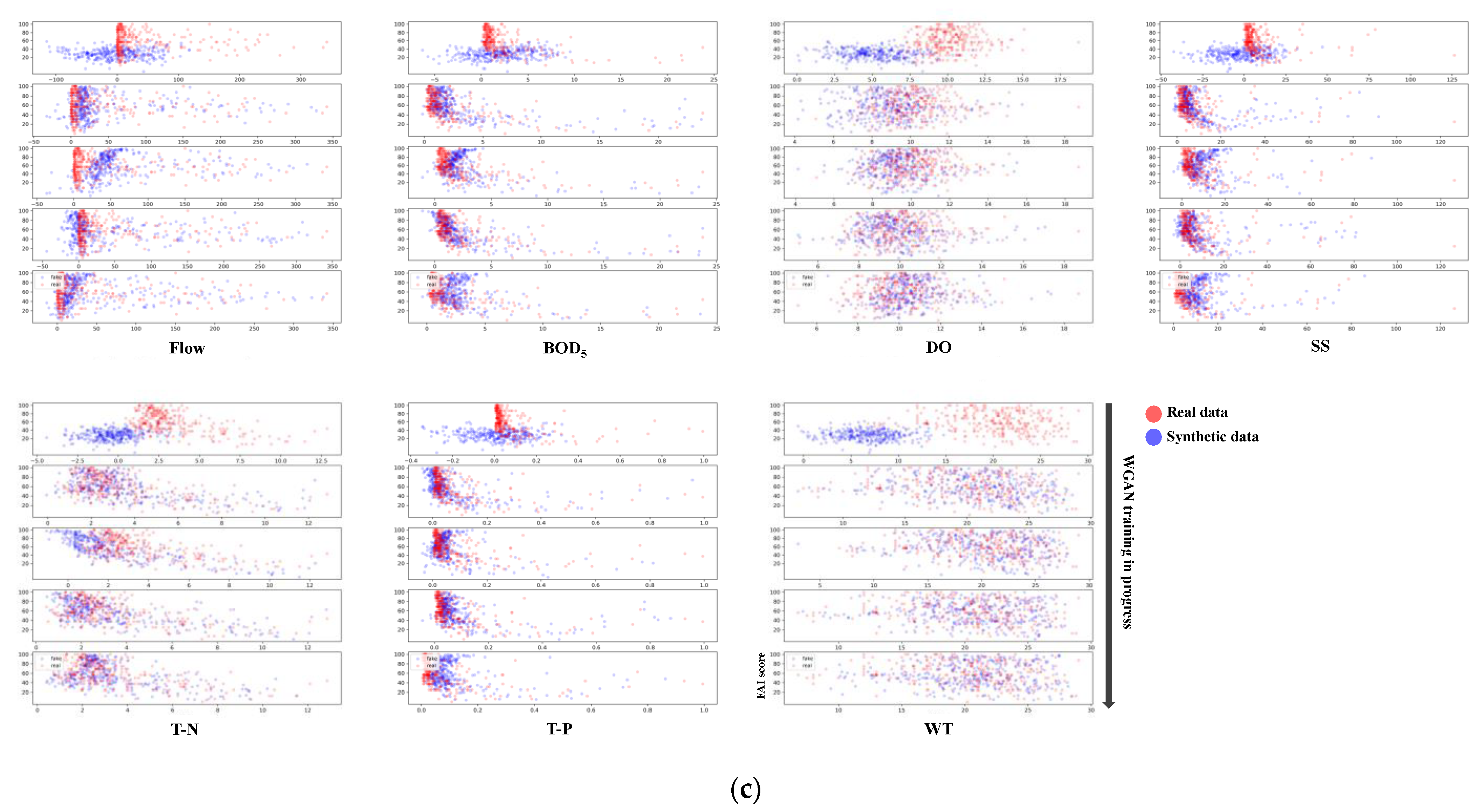
3.2. Correlation Analysis and WGAN-Based Data Augmentation Results
3.3. Comparison of Validation Results of ML Models
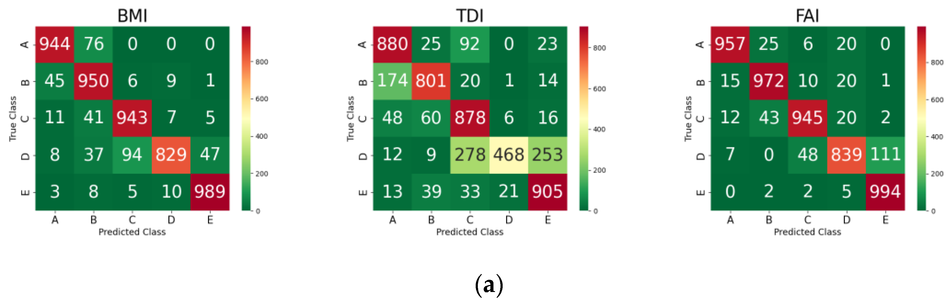
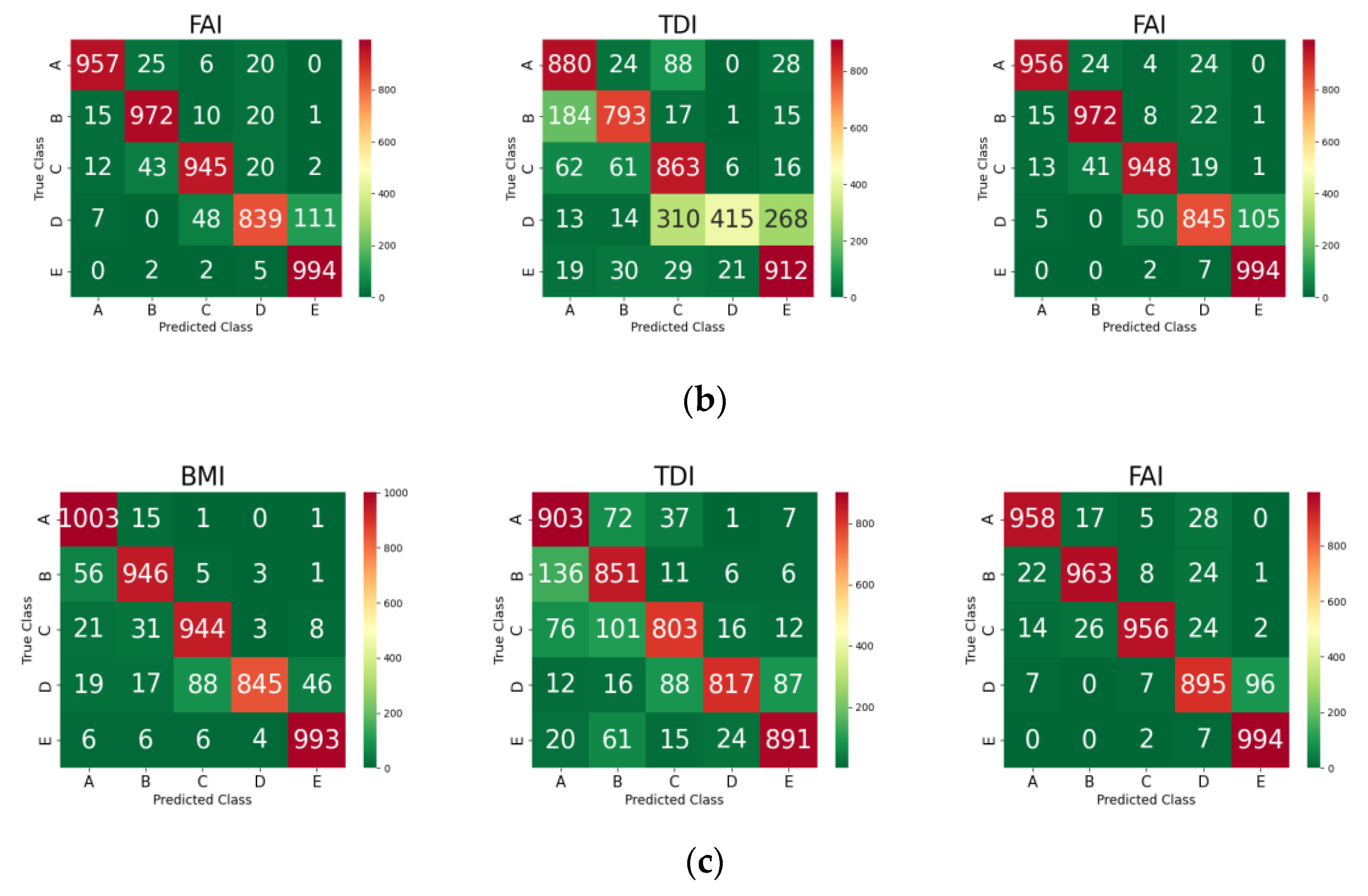
3.4. Grade Prediction of Each AEH Index for Test Set Using the ML Models
4. Conclusions
Author Contributions
Funding
Institutional Review Board Statement
Informed Consent Statement
Data Availability Statement
Conflicts of Interest
References
- Peters, N.E.; Meybeck, M.; Chapman, D.V. Effects of Human Activities on Water Quality. Encycl. Hydrol. Sci. 2005. [Google Scholar] [CrossRef]
- Delpla, I.; Jung, A.V.; Baures, E.; Clement, M.; Thomas, O. Impacts of climate change on surface water quality in relation to drinking water production. Environ. Int. 2009, 35, 1225–1233. [Google Scholar] [CrossRef] [PubMed]
- Qiu, J.; Shen, Z.; Leng, G.; Xie, H.; Hou, X.; Wei, G. Impacts of climate change on watershed systems and potential adaptation through BMPs in a drinking water source area. J. Hydrol. 2019, 573, 123–135. [Google Scholar] [CrossRef]
- Liao, H.; Sarver, E.; Krometis, L.A.H. Interactive effects of water quality, physical habitat, and watershed anthropogenic activities on stream ecosystem health. Water Res. 2018, 130, 69–78. [Google Scholar] [CrossRef] [PubMed]
- Reid, A.J.; Carlson, A.K.; Creed, I.F.; Eliason, E.J.; Gell, P.A.; Johnson, P.T.J.; Kidd, K.A.; MacCormack, T.J.; Olden, J.D.; Ormerod, S.J.; et al. Emerging threats and persistent conservation challenges for freshwater biodiversity. Biol. Rev. 2019, 94, 849–873. [Google Scholar] [CrossRef] [PubMed]
- Baron, J.S.; Poff, N.L.; Angermeier, P.L.; Dahm, C.N.; Gleick, P.H.; Hairston, N.G.; Jackson, R.B.; Johnston, C.A.; Richter, B.D.; Steinman, A.D. Meeting Ecological and Societal Needs for Freshwater. Ecol. Appl. 2002, 12, 1247. [Google Scholar] [CrossRef]
- Zhao, C.; Shao, N.; Yang, S.; Ren, H.; Ge, Y.; Zhang, Z.; Zhao, Y.; Yin, X. Integrated assessment of ecosystem health using multiple indicator species. Ecol. Eng. 2019, 130, 157–168. [Google Scholar] [CrossRef]
- Karr, J.R. Assessment of Biotic Integrity Using Fish Communities. Fisheries 1981, 6, 21–27. [Google Scholar] [CrossRef]
- Ohio EPA. Biological Criteria for the Protection of Aquatic Life: Standardized Biological Field Sampling and Laboratory Methods for Aseessing Fish and Macroinvertebrate Communities; Tech. Rept. EAS/2015-06-01; revised 26 June 2015; Ohio Environmental Protection Agency, Division of Water Quality Monitoring and Assessment: Columbus, OH, USA, 1987; Volume III, p. 120.
- U.S. EPA. Biological Assessments and Criteria: Crucial Components of Water Quality Programs; EPA 822-F-02-006; U.S. Environmental Protection Agency Office of Water: Washington, DC, USA, 2002.
- National Institute of Environmental Research. Biomonitoring Survey and Assessment Manual; National Institute of Environmental Research: Incheon, Korea, 2016; p. 372.
- Chen, H.; Ma, L.; Guo, W.; Yang, Y.; Guo, T.; Feng, C. Linking Water Quality and Quantity in Environmental Flow Assessment in Deteriorated Ecosystems: A Food Web View. PLoS ONE 2013, 8, e70537. [Google Scholar] [CrossRef]
- Liu, Y.; Zhang, T.; Kang, A.; Li, J.; Lei, X. Research on Runoff Simulations Using Deep-Learning Methods. Sustainability 2021, 13, 1336. [Google Scholar] [CrossRef]
- Lee, J.; Lee, S.; Hong, J.; Lee, D.; Bae, J.H.; Yang, J.E.; Kim, J.; Lim, K.J. Evaluation of Rainfall Erosivity Factor Estimation Using Machine and Deep Learning Models. Water 2021, 13, 382. [Google Scholar] [CrossRef]
- Hong, J.; Lee, S.; Bae, J.H.; Lee, J.; Park, W.J.; Lee, D.; Kim, J.; Lim, K.J. Development and evaluation of the combined machine learning models for the prediction of dam inflow. Water 2020, 12, 2927. [Google Scholar] [CrossRef]
- Nourani, V.; Gokcekus, H.; Gelete, G. Estimation of Suspended Sediment Load Using Artificial Intelligence-Based Ensemble Model. Complexity 2021, 2021, 6633760. [Google Scholar] [CrossRef]
- Al-adhaileh, M.H. Modelling and Prediction of Water Quality by Using Artificial Intelligence. Sustainability 2021, 13, 4259. [Google Scholar] [CrossRef]
- Woo, S.Y.; Jung, C.G.; Lee, J.W.; Kim, S.J. Evaluation of watershed scale aquatic ecosystem health by SWAT modeling and random forest technique. Sustainability 2019, 11, 3397. [Google Scholar] [CrossRef]
- Xue, H.; Zheng, B.; Meng, F.; Wang, Y.; Zhang, L. Assessment of Aquatic Ecosystem Health of the Wutong River Based on Benthic Diatoms. Water 2019, 11, 727. [Google Scholar] [CrossRef]
- Goodfellow, I.; Pouget-Abadie, J.; Mirza, M.; Xu, B.; Warde-Farley, D.; Ozair, S.; Courville, A.; Bengio, Y. Generative adversarial nets. In Proceedings of the 27th International conference on Neural Information Processing Systems; MIT Press: Cambridge, MA, USA, 2014; Volume 2, pp. 2672–2680. [Google Scholar]
- Frid-Adar, M.; Diamant, I.; Klang, E.; Amitai, M.; Goldberger, J.; Greenspan, H. GAN-based synthetic medical image augmentation for increased CNN performance in liver lesion classification. Neurocomputing 2018, 321, 321–331. [Google Scholar] [CrossRef]
- Lu, C.; Jeric, D.; Rustia, A.; Lin, T.; Rustia, A.; Lin, T.; Lu, C.; Jeric, D.; Rustia, J.A.; Lin, T.; et al. Generative Adversarial Networks (GAN); Image augmentation; Integrated pest management. IFAC Pap. 2019, 52, 1–5. [Google Scholar] [CrossRef]
- Goodfellow, I. NIPS 2016 Tutorial: Generative Adversarial Networks. arXiv 2016, arXiv:1701.00160. [Google Scholar]
- Arjovsky, M.; Chintala, S.; Bottou, L. Wasserstein generative adversarial networks. In Proceedings of the 34th International Conference on Machine Learning, Sydney, Australia, 6–11 August 2017; Volume 70, pp. 214–223. [Google Scholar]
- Wei, X.; Gong, B.; Liu, Z.; Lu, W.; Wang, L. Improving the improved training of wasserstein gans: A consistency term and its dual effect. arXiv 2018, arXiv:1803.01541. [Google Scholar]
- Jiang, C.; Zhang, Q.; Ge, Y.; Liang, D.; Yang, Y.; Liu, X.; Zheng, H.; Hu, Z. Wasserstein generative adversarial networks for motion artifact removal in dental CT imaging. In Proceedings of the Medical Imaging 2019: Physics of Medical Imaging. International Society for Optics and Photonics, San Diego, CA, USA, 17–20 February 2019; Volume 10948. [Google Scholar] [CrossRef]
- Xia, H.; Liu, C. Remote Sensing Image Deblurring Algorithm Based on WGAN. In Proceedings of the International Conference on Service-Oriented Computing, Hangzhou, China, 12–15 November 2018; Springer: Cham, Switzerland, 2018; pp. 113–125. [Google Scholar]
- Cho, Y.; Park, M.; Shin, K.; Choi, H.; Kim, S.; Yu, S. A Study on Grade Classification for Improvement of Water Quality and Water Quality Characteristics in the Han River Watershed Tributaries. J. Environ. Impact Assess. 2019, 28, 215–230. [Google Scholar]
- Lee, S.; Shin, J.Y.; Lee, G.; Sung, Y.; Kim, K.; Lim, K.J.; Kim, J. Analysis of water pollutant load characteristics and its contributions during dry season: Focusing on major streams inflow into South-Han river of Chungju-dam downstream. J. Korean Soc. Environ. Eng. 2018, 40, 247–257. [Google Scholar] [CrossRef][Green Version]
- Fan, J.; Li, M.; Guo, F.; Yan, Z.; Zheng, X.; Zhang, Y.; Xu, Z.; Wu, F. Priorization of river restoration by coupling soil and water assessment tool (SWAT) and support vector machine (SVM) models in the Taizi river basin, northern China. Int. J. Environ. Res. Public Health 2018, 15, 2090. [Google Scholar] [CrossRef]
- Kemp, P.; Sear, D.; Collins, A.; Naden, P.; Jones, I. The impacts of fine sediment on riverine fish. Hydrol. Process. 2011, 25, 1800–1821. [Google Scholar] [CrossRef]
- Chawla, N.V.; Japkowicz, N.; Kotcz, A. Editorial: Special Issue on Learning from Imbalanced Data Sets. ACM SIGKDD Explor. Newsl. 2004, 6, 1–6. [Google Scholar] [CrossRef]
- Arjovsky, M.; Bottou, L. Towards principled methods for training generative adversarial networks. arXiv 2017, arXiv:1701.04862. [Google Scholar]
- Srivastava, N.; Hinton, G.; Krizhevsky, A.; Sutskever, I.; Salakhutdinov, R. Dropout: A Simple Way to Prevent Neural Networks from Overfitting. J. Mach. Learn. Res. 2014, 15, 1929–1958. [Google Scholar]
- Vapnik, V.N. An overview of statistical learning theory. IEEE Trans. Neural Netw. 1999, 10, 988–999. [Google Scholar] [CrossRef]
- Quinlan, J.R. Induction of decision trees. Mach. Learn. 1986, 1, 81–106. [Google Scholar] [CrossRef]
- Altman, N.S. An introduction to kernel and nearest-neighbor nonparametric regression. Am. Stat. 1992, 46, 175–185. [Google Scholar] [CrossRef]
- LEO Breiman Random forests. Random For. 2001, 1–122. [CrossRef]
- Friedman, J.H. Greedy function approximation: A gradient boosting machine. Ann. Stat. 1999, 29, 1189–1232. [Google Scholar] [CrossRef]
- Chen, T.; Guestrin, C. XGBoost: A scalable tree boosting system. In Proceedings of the 22nd Acm Sigkdd International Conference on Knowledge Discovery and Data Mining, San Francisco, CA, USA, 13–17 August 2016; pp. 785–794. [Google Scholar] [CrossRef]
- Bae, J.H.; Han, J.; Lee, D.; Yang, J.E.; Kim, J.; Lim, K.J.; Ne, J.C.; Jang, W.S. Evaluation of Sediment Trapping Efficiency of Vegetative Filter Strips Using Machine Learning Models. Sustainability 2019, 11, 7212. [Google Scholar] [CrossRef]
- Choi, J. A study on the standardization strategy for building of learning data set for machine learning applications. J. Digit. Converg. 2018, 16, 205–212. [Google Scholar] [CrossRef]
- Fushiki, T. Estimation of prediction error by using K-fold cross-validation. Stat. Comput. 2011, 21, 137–146. [Google Scholar] [CrossRef]
- Molinaro, A.M.; Simon, R.; Pfeiffer, R.M. Prediction error estimation: A comparison of resampling methods. Bioinformatics 2005, 21, 3301–3307. [Google Scholar] [CrossRef]
- Singh, G.; Panda, R.K. Daily sediment yield modeling with artificial neural network using 10-fold nross validation method: A small agricultural watershed, Kapgari, India. Int. J. Earth Sci. Eng. 2011, 4, 443–450. [Google Scholar]
- Sammut, C.; Webb, G.I. Encyclopedia of Machine Learning; Springer Science & Business Media: Berlin/Heidelberg, Germany, 2011; ISBN 0387307680. [Google Scholar]
- Musumba, M.; Fatema, N.; Kibriya, S. Prevention Is Better Than Cure: Machine Learning Approach to Conflict Prediction in Sub-Saharan Africa. Sustainability 2021, 13, 7366. [Google Scholar] [CrossRef]
- Taner, A.; Öztekin, Y.B.; Duran, H. Performance Analysis of Deep Learning CNN Models for Variety Classification in Hazelnut. Sustainability 2021, 13, 6527. [Google Scholar] [CrossRef]
- Zheng, A. Evaluating Machine Learning Algorithms; O’Reilly, Media Inc.: Sebastopol, CA, USA, 2015; ISBN 9781491932469. [Google Scholar]
- Ibrahim, M.; Torki, M.; El-Makky, N. Imbalanced Toxic Comments Classification Using Data Augmentation and Deep Learning. In Proceedings of the 2018 17th IEEE International Conference on Machine Learning and Applications (ICMLA), Orlando, FL, USA, 17–20 December 2018; pp. 875–878. [Google Scholar]
- Woo, S.Y.; Jung, C.G.; Kim, J.U.; Kim, S.J. Assessment of climate change impact on aquatic ecology health indices in Han river basin using SWAT and random forest. J. Korea Water Resour. Assoc. 2018, 51, 863–874. [Google Scholar] [CrossRef]
- Kim, M.; Yoon, C.G.; Rhee, H.-P.; Soon-Jin, H.; Lee, S.-W. A Study on Predicting TDI ( Trophic Diatom Index ) in tributaries of Han river basin using Correlation-based Feature Selection technique and Random Forest algorithm. J. Korean Soc. Water Environ. 2019, 5, 432–438. [Google Scholar] [CrossRef]
- Griffiths, W.H.; Walton, B.D. The Effects of Sedimentation on the Aquatic Biota. In Alberta Oil Sands Environmental Research Program; Report No. 35; Oil Sands Reseach and Information Network; University of Alberta: Edmonton, AB, Canada, 1978. [Google Scholar] [CrossRef]
- Kong, D.; Son, S.; Hwang, S.; Won, D.H.; Kim, M.C.; Park, J.H.; Jeon, T.S.; Lee, J.E.; Kim, J.H.; Kim, J.S.; et al. Development of Benthic Macroinvertebrates Index (BMI) for Biological Assessment on Stream Environment. J. Korean Soc. Water Environ. 2018, 34, 183–201. [Google Scholar] [CrossRef]
- Newcombe, C.P.; Macdonald, D.D. Effects of Suspended Sediments on Aquatic Ecosystems. N. Am. J. Fish. Manag. 1991, 11, 72–82. [Google Scholar] [CrossRef]
- Sun, Q.; Wang, W.; Gan, A. A method to accelerate the training of WGAN. In Proceedings of the 2018 5th International Conference on Information Science and Control Engineering (ICISCE), Zhengzhou, China, 20–22 July 2018; pp. 2–5. [Google Scholar] [CrossRef]
- Longadge, R.; Dongre, S. Class Imbalance Problem in Data Mining Review. Int. J. Comput. Sci. Netw. 2013, 2. [Google Scholar]
- Gulrajani, I.; Ahmed, F.; Arjovsky, M.; Dumoulin, V.; Courville, A. Improved training of wasserstein GANs. Adv. Neural Inf. Process. Syst. 2017, 2017, 5768–5778. [Google Scholar]
- More, A.S.; Rana, D.P. Review of random forest classification techniques to resolve data imbalance. In Proceedings of the 2017 1st International Conference on Intelligent Systems and Information Management (ICISIM), Aurangabad, India, 5–6 October 2017; IEEE: Manhattan, NY, USA, 2017; pp. 72–78. [Google Scholar]
- Zhang, M.; Shi, W.; Xu, Z. Systematic comparison of five machine-learning models in classification and interpolation of soil particle size fractions using different transformed data. Hydrol. Earth Syst. Sci. 2020, 24, 2505–2526. [Google Scholar] [CrossRef]
- Patle, A.; Chouhan, D.S. SVM kernel functions for classification. In Proceedings of the 2013 International Conference on Advances in Technology and Engineering (ICATE), Mumbai, India, 23–25 January 2013; pp. 1–9. [Google Scholar]
- Bhatia, S.; Dahyot, R. Using WGAN for improving imbalanced classification performance. CEUR Workshop Proc. 2019, 2563, 365–375. [Google Scholar]
- Han, X.; Zhang, L.; Zhou, K.; Wang, X. Deep learning framework DNN with conditional WGAN for protein solubility prediction. arXiv 2018, arXiv:1811.07140. [Google Scholar]
- Zhang, L.; Yang, H.; Jiang, Z. Imbalanced biomedical data classification using self-adaptive multilayer ELM combined with dynamic GAN. Biomed. Eng. Online 2018, 17, 1–21. [Google Scholar] [CrossRef]


| Indices | A (Very Good) | B (Good) | C (Fair) | D (Poor) | E (Very Poor) |
|---|---|---|---|---|---|
| BMI | ≥80 | ≥65 | ≥50 | ≥35 | <35 |
| TDI | ≥90 | ≥70 | ≥50 | ≥30 | <30 |
| FAI | ≥80 | ≥60 | ≥40 | ≥20 | <20 |
| Target | Description | Input | ||||||
|---|---|---|---|---|---|---|---|---|
| Flow (m3/sec) | BOD5 (mg/L) | DO (mg/L) | SS (mg/L) | TN (mg/L) | TP (mg/L) | WT (°C) | ||
| BMI | Mean | 41.22 | 1.92 | 10.10 | 6.76 | 3.088 | 0.066 | 20.33 |
| Min, Max | 0.006, 544.4 | 0.2, 25.8 | 5.1, 17.74 | 0.2, 67.0 | 0.534, 16.0 | 0.003, 1.0 | 5.2, 30.2 | |
| TDI | Mean | 37.12 | 1.88 | 9.87 | 7.00 | 3.297 | 0.079 | 20.17 |
| Min, Max | 0.024, 424.8 | 0.3, 25.8 | 6.34, 14.6 | 0.1, 140.5 | 0.467, 18.5 | 0.004, 2.2 | 6.6, 28.7 | |
| FAI | Mean | 39.10 | 2.18 | 10.08 | 8.18 | 3.369 | 0.078 | 20.17 |
| Min, Max | 0.012, 342.7 | 0.1, 23.8 | 5.1, 18.7 | 0.1, 126.3 | 0.467, 12.9 | 0.004, 1.0 | 6.8, 29.0 | |
| Indices | A | B | C | D | E | Total |
|---|---|---|---|---|---|---|
| BMI | 171 | 66 | 45 | 35 | 22 | 339 |
| TDI | 65 | 93 | 68 | 43 | 50 | 319 |
| FAI | 70 | 63 | 82 | 49 | 18 | 282 |
| ML Models | Module | Function | Notation |
|---|---|---|---|
| Support Vector Machine | Sklearn.svm | SVC | SVM |
| Decision Tree | Sklearn.tree | DecisionTreeClassifier | DT |
| K-Nearest Neighbors | Sklearn.neighbors | KNeighborsClassifier | KNN |
| Random Forest | Sklearn.ensemble | RandomForestClassifier | RF |
| Gradient Boosting | Sklearn.ensemble | GradientBoostingClassifier | GB |
| eXtreme Gradient Boost | xgboost.xgb | XGBClassifier | XGB |
| Grade | BMI | TDI | FAI | |||
|---|---|---|---|---|---|---|
| Augmented | WGAN-Based | Augmented | WGAN-Based | Augmented | WGAN-Based | |
| A | 6916 | 7087 | 5190 | 5255 | 5000 | 5070 |
| B | 4935 | 5001 | 5398 | 5491 | 5000 | 5063 |
| C | 4067 | 4112 | 5878 | 5946 | 4617 | 4699 |
| D | 3500 | 3535 | 3615 | 3658 | 5383 | 5432 |
| E | 5582 | 5604 | 4919 | 4969 | 5000 | 5018 |
| Total | 25,000 | 25,339 | 25,000 | 25,319 | 25,000 | 25,282 |
| Metric | Grade | SVM | RF | DT | KNN | GB | XGB |
|---|---|---|---|---|---|---|---|
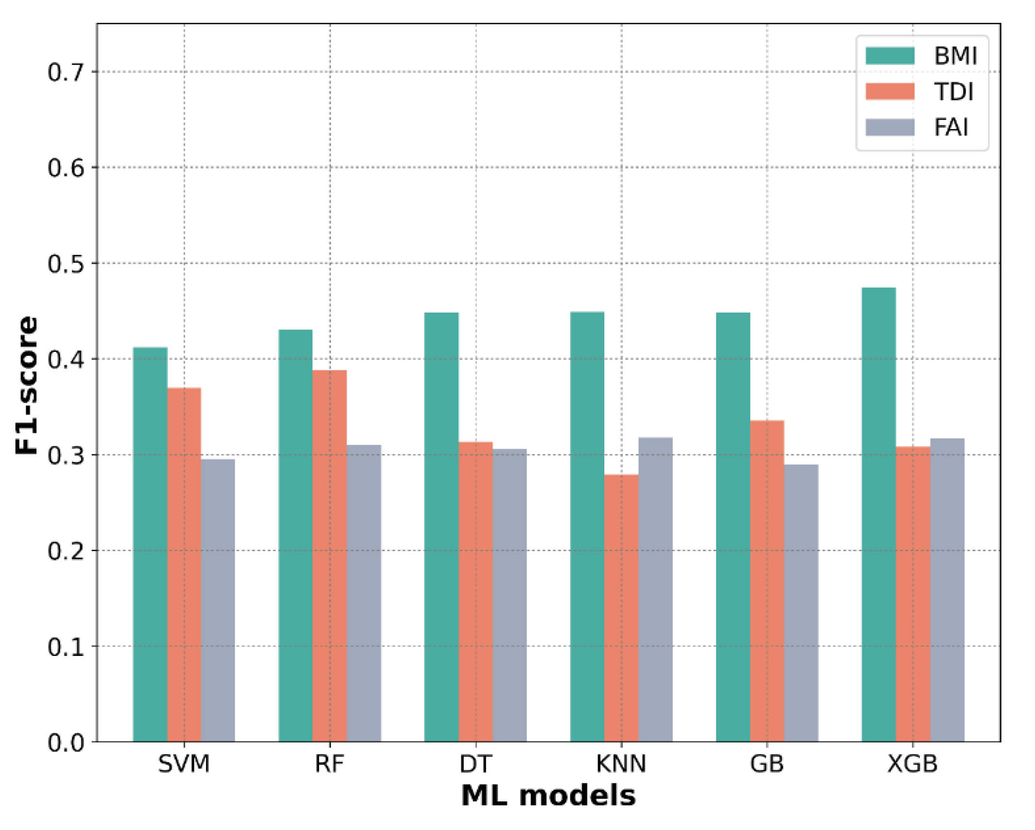
| F1-score | BMI | 0.412 | 0.430 | 0.448 | 0.449 | 0.448 | 0.475 |
| TDI | 0.370 | 0.388 | 0.313 | 0.279 | 0.335 | 0.308 | |
| FAI | 0.296 | 0.310 | 0.306 | 0.318 | 0.290 | 0.317 | |
| Avg | 0.359 | 0.376 | 0.356 | 0.349 | 0.358 | 0.367 |
| Metric | Grade | RF | XGB | SVM | |||
|---|---|---|---|---|---|---|---|
| Raw | WGAN-Based | Raw | WGAN-Based | Raw | WGAN-Based | ||
| F1-score | BMI | 0.430 | 0.973 | 0.475 | 0.976 | 0.412 | 0.964 |
| TDI | 0.388 | 0.943 | 0.308 | 0.946 | 0.370 | 0.913 | |
| FAI | 0.310 | 0.944 | 0.317 | 0.955 | 0.296 | 0.982 | |
| Avg | 0.376 | 0.953 | 0.367 | 0.959 | 0.359 | 0.953 | |
| Model | Grade | BMI | TDI | FAI | |||||||||
|---|---|---|---|---|---|---|---|---|---|---|---|---|---|
| P | R | F1 | S | P | R | F1 | S | P | R | F1 | S | ||
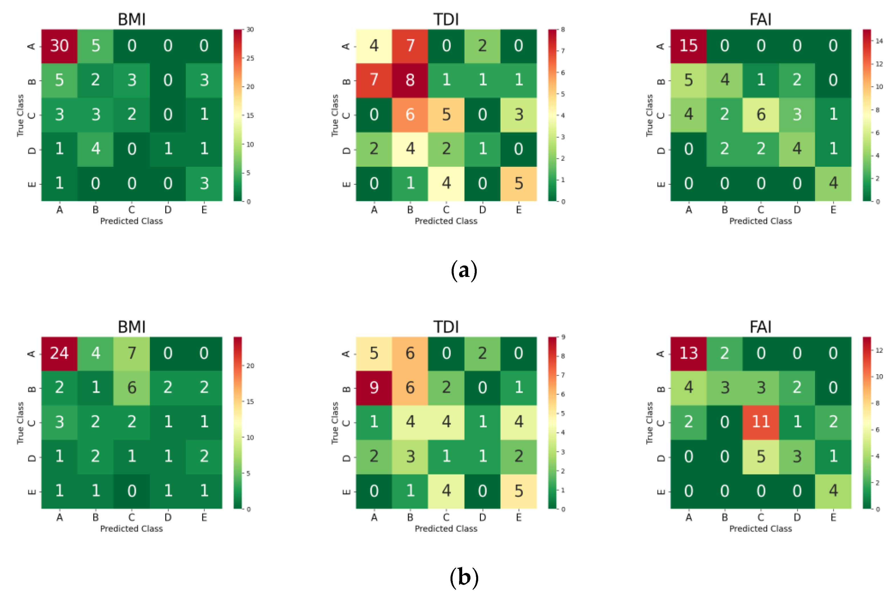
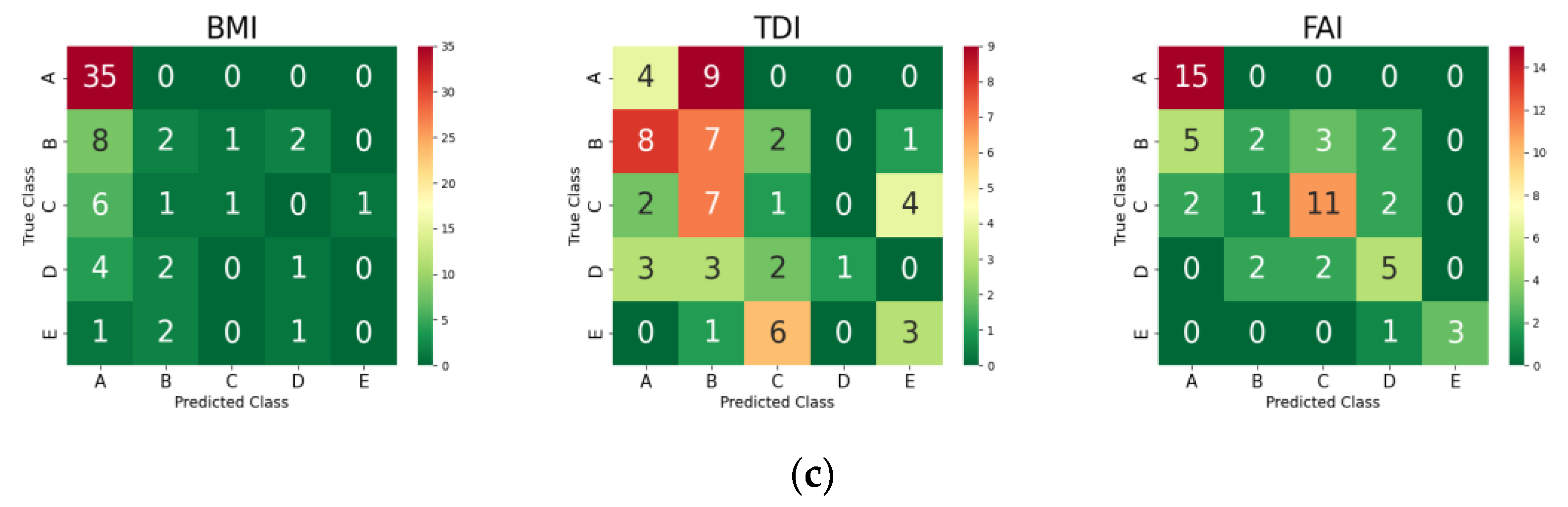
| RF | A | 0.75 | 0.86 | 0.80 | 35 | 0.31 | 0.31 | 0.31 | 13 | 0.62 | 1 | 0.77 | 15 |
| B | 0.14 | 0.15 | 0.15 | 13 | 0.31 | 0.44 | 0.36 | 18 | 0.50 | 0.33 | 0.40 | 12 | |
| C | 0.40 | 0.22 | 0.29 | 9 | 0.42 | 0.36 | 0.38 | 14 | 0.67 | 0.38 | 0.48 | 16 | |
| D | 1 | 0.14 | 0.25 | 7 | 0.25 | 0.11 | 0.15 | 9 | 0.44 | 0.44 | 0.44 | 9 | |
| E | 0.38 | 0.75 | 0.50 | 4 | 0.56 | 0.50 | 0.53 | 10 | 0.67 | 1 | 0.80 | 4 | |
| Avg | 0.59 | 0.56 | 0.53 | 68 | 0.36 | 0.36 | 0.35 | 64 | 0.58 | 0.59 | 0.56 | 56 | |
| XGB | A | 0.77 | 0.69 | 0.73 | 35 | 0.29 | 0.38 | 0.33 | 13 | 0.68 | 0.87 | 0.76 | 15 |
| B | 0.10 | 0.08 | 0.09 | 13 | 0.30 | 0.33 | 0.32 | 18 | 0.60 | 0.25 | 0.35 | 12 | |
| C | 0.12 | 0.22 | 0.16 | 9 | 0.36 | 0.29 | 0.32 | 14 | 0.58 | 0.69 | 0.63 | 16 | |
| D | 0.20 | 0.14 | 0.17 | 7 | 0.25 | 0.11 | 0.15 | 9 | 0.50 | 0.33 | 0.40 | 9 | |
| E | 0.17 | 0.25 | 0.20 | 4 | 0.42 | 0.50 | 0.45 | 10 | 0.57 | 1 | 0.73 | 4 | |
| Avg | 0.46 | 0.43 | 0.44 | 68 | 0.32 | 0.33 | 0.32 | 64 | 0.60 | 0.61 | 0.58 | 56 | |
| SVM | A | 0.65 | 1 | 0.79 | 35 | 0.24 | 0.31 | 0.27 | 13 | 0.68 | 1 | 0.81 | 15 |
| B | 0.29 | 0.15 | 0.20 | 13 | 0.26 | 0.39 | 0.31 | 18 | 0.40 | 0.17 | 0.24 | 12 | |
| C | 0.50 | 0.11 | 0.18 | 9 | 0.09 | 0.07 | 0.08 | 14 | 0.69 | 0.69 | 0.69 | 16 | |
| D | 0.25 | 0.14 | 0.18 | 7 | 1 | 0.11 | 0.20 | 9 | 0.50 | 0.56 | 0.53 | 9 | |
| E | 0 | 0 | 0 | 4 | 0.38 | 0.30 | 0.33 | 10 | 1 | 0.75 | 0.86 | 4 | |
| Avg | 0.48 | 0.57 | 0.49 | 68 | 0.34 | 0.25 | 0.24 | 64 | 0.62 | 0.64 | 0.61 | 56 | |
| Model | Grade | BMI | TDI | FAI | |||||||||
|---|---|---|---|---|---|---|---|---|---|---|---|---|---|
| P | R | F1 | S | P | R | F1 | S | P | R | F1 | S | ||
| RF | A | 0.93 | 0.93 | 0.93 | 1020 | 0.78 | 0.86 | 0.82 | 1020 | 0.97 | 0.95 | 0.96 | 1008 |
| B | 0.85 | 0.94 | 0.89 | 1011 | 0.86 | 0.79 | 0.82 | 1010 | 0.93 | 0.95 | 0.94 | 1018 | |
| C | 0.90 | 0.94 | 0.92 | 1007 | 0.67 | 0.87 | 0.76 | 1008 | 0.93 | 0.92 | 0.93 | 1022 | |
| D | 0.97 | 0.82 | 0.89 | 1015 | 0.94 | 0.46 | 0.62 | 1020 | 0.93 | 0.83 | 0.88 | 1005 | |
| E | 0.95 | 0.97 | 0.96 | 1015 | 0.75 | 0.90 | 0.81 | 1011 | 0.90 | 0.99 | 0.94 | 1003 | |
| Avg | 0.92 | 0.92 | 0.92 | 5068 | 0.80 | 0.78 | 0.77 | 5069 | 0.93 | 0.93 | 0.93 | 5056 | |
| XGB | A | 0.93 | 0.96 | 0.94 | 1020 | 0.76 | 0.86 | 0.81 | 1020 | 0.97 | 0.95 | 0.96 | 1008 |
| B | 0.87 | 0.94 | 0.91 | 1011 | 0.86 | 0.79 | 0.82 | 1010 | 0.94 | 0.95 | 0.95 | 1018 | |
| C | 0.90 | 0.91 | 0.91 | 1007 | 0.66 | 0.86 | 0.75 | 1008 | 0.94 | 0.93 | 0.93 | 1022 | |
| D | 0.95 | 0.82 | 0.88 | 1015 | 0.94 | 0.41 | 0.57 | 1020 | 0.92 | 0.84 | 0.88 | 1005 | |
| E | 0.95 | 0.97 | 0.96 | 1015 | 0.74 | 0.90 | 0.81 | 1011 | 0.90 | 0.99 | 0.94 | 1003 | |
| Avg | 0.92 | 0.92 | 0.92 | 5068 | 0.79 | 0.76 | 0.75 | 5069 | 0.93 | 0.93 | 0.93 | 5056 | |
| SVM | A | 0.91 | 0.98 | 0.94 | 1020 | 0.79 | 0.89 | 0.83 | 1020 | 0.96 | 0.95 | 0.95 | 1008 |
| B | 0.93 | 0.94 | 0.93 | 1011 | 0.77 | 0.84 | 0.81 | 1010 | 0.96 | 0.95 | 0.95 | 1018 | |
| C | 0.90 | 0.94 | 0.92 | 1007 | 0.84 | 0.80 | 0.82 | 1008 | 0.98 | 0.94 | 0.96 | 1022 | |
| D | 0.99 | 0.83 | 0.90 | 1015 | 0.95 | 0.80 | 0.87 | 1020 | 0.92 | 0.89 | 0.90 | 1005 | |
| E | 0.95 | 0.98 | 0.96 | 1015 | 0.89 | 0.88 | 0.88 | 1011 | 0.91 | 0.99 | 0.95 | 1003 | |
| Avg | 0.94 | 0.93 | 0.93 | 5068 | 0.85 | 0.84 | 0.84 | 5069 | 0.94 | 0.94 | 0.94 | 5056 | |
Publisher’s Note: MDPI stays neutral with regard to jurisdictional claims in published maps and institutional affiliations. |
© 2021 by the authors. Licensee MDPI, Basel, Switzerland. This article is an open access article distributed under the terms and conditions of the Creative Commons Attribution (CC BY) license (https://creativecommons.org/licenses/by/4.0/).
Share and Cite
Lee, S.; Kim, J.; Lee, G.; Hong, J.; Bae, J.H.; Lim, K.J. Prediction of Aquatic Ecosystem Health Indices through Machine Learning Models Using the WGAN-Based Data Augmentation Method. Sustainability 2021, 13, 10435. https://doi.org/10.3390/su131810435
Lee S, Kim J, Lee G, Hong J, Bae JH, Lim KJ. Prediction of Aquatic Ecosystem Health Indices through Machine Learning Models Using the WGAN-Based Data Augmentation Method. Sustainability. 2021; 13(18):10435. https://doi.org/10.3390/su131810435
Chicago/Turabian StyleLee, Seoro, Jonggun Kim, Gwanjae Lee, Jiyeong Hong, Joo Hyun Bae, and Kyoung Jae Lim. 2021. "Prediction of Aquatic Ecosystem Health Indices through Machine Learning Models Using the WGAN-Based Data Augmentation Method" Sustainability 13, no. 18: 10435. https://doi.org/10.3390/su131810435
APA StyleLee, S., Kim, J., Lee, G., Hong, J., Bae, J. H., & Lim, K. J. (2021). Prediction of Aquatic Ecosystem Health Indices through Machine Learning Models Using the WGAN-Based Data Augmentation Method. Sustainability, 13(18), 10435. https://doi.org/10.3390/su131810435