Abstract
Mobility is a must for human life on this planet, because important activities like working or shopping cannot be done from home for everyone. Present modes of transports contributes significantly to green house gas emissions while the efforts to reduce these emissions can be improved in many countries. Pathways to a more sustainable form of mobility can be modelled using travel demand models to aid decision makers. However, to project human behavior into the future one should analyze the changes in the past to understand the drivers in mobility change. Mobility surveys provide sets of activity diaries, which show changes in travel behavior over time. Those activity diaries are one of the inputs in activity-based demand generation models like travel activity pattern simulation (TAPAS). This paper shows a method of using probability distributions between person and diary groups. It offers an opportunity for an increased heterogeneity in travel behavior without sacrificing too much accuracy. Additionally it will present the use case of temporal back- and forecasting of changes in activity choices of existing mobility survey data. The results show the possibilities within this approach together with its limits and pitfalls.
1. Introduction
Mobility is needed in any form of human society. Although the sectors of energy generation and food production are transforming towards sustainability for decades, the mobility sector in the industrialized countries is still heavily dependent on individual modes of transports, namely cars and trucks. In Germany, the total amount of carbon dioxide emissions in the transportation sector has not changed from 1990 to 2019, while most other sectors have significantly reduced their emissions [1]. To be able to form a sustainable future for the mobility sector decision makers have to know, how the usage of modes of transportation has changed and is changing. One way to support the decision makers to forecast travel demand by travel demand generation models, which simulate the demand of mobility for a given set of parameters in a specific region. The outcome of such models represents the reaction of the population to hypothetical introduced measures resulting in changes of trips and their length, performed activity, and used mode of transport. In case of car trips, these values can be used to calculate the CO2 emission and traffic jams. A case of rebound effects regarding fuel efficiency improvements and the following increase in car traffic demand is shown and discussed in [2]. Because human behavior is not strictly logical or economical in every way these models have to deal with many uncertainties and cope with the errors statistically. Therefore, understanding why people leave their homes, how this behavior has changed over the years and how to forecast it is crucial for the quality of travel demand modeling to show pathways to a sustainable transport system with respect to the mobility needs. The Mobilität in Deutschland (MiD, Mobility in Germany) survey tracks mobility patterns of the German population since 2002 [3]. With its second [4] and third instalment [5] one can see a change in travel behavior over time. A summary of the development of these surveys can be seen in the MiD time series report [6].
Figure 1 shows that from 2002 to 2017 the number of trips decreased with a slight bump in 2008. Looking at the specific activity categories the biggest changes are found in shopping, free time, personal matters and work. According to the MiD time series report [6] the increase in work-related trips is not because of more trips to work but rather business trips during work. One factor in the surge of business trips is assumed to be because of courier and parcel services. The MiD is unclear about the correlation between the reduction in shopping trips due to e-commerce (together with the increase in business trips) but states structural changes of shopping opportunities. Smaller stores like bakeries and butcher’s shops disappeared or were integrated into bigger supermarkets which led to fewer trips ([6], pp. 59–62).
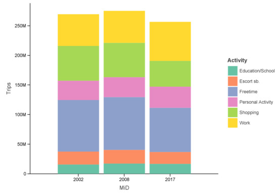
Figure 1.
Number of trips per day ([6], compare p. 60 Figure 35).
Activity diaries play an important role in modeling travel behavior. Activity-based demand generation models like travel activity pattern simulation (TAPAS) [7,8,9,10] rely on large datasets of mobility surveys such as the MiD. In general, travel demand models separate their simulation into four sub-models: First, trip generation, where private trips with specific purposes are generated due to their socio-economic status, age, employment, etc. Second, trip distribution: here a location choice for the desired trip purpose is done based on accessibility, type of location, personal constraints, capacity, and occupancy. The third step is the choice of mode of transportation, which is often integrated in location choice, because one cannot exist without the other. The mode choice highly depends on availability of the mode, pricing, travel time, and trip purpose. The fourth and last step is called traffic assignment, where the routes for each trip is calculated and capacity constraints of the roads and buses are taken into account.
In this paper, we present an enhanced method using probability distributions based on trip purpose hierarchies. This addresses the first step in the previously described four-step-model. A similar approach was shown in [10,11,12,13] but with a different set of group divisions. Furthermore, this previous work could not analyze the performance of the proposed approach due to the lack of consecutive installments of their primary data source. We test the accuracy of this concept while obtaining more heterogeneity in modeled travel behavior. Because it is extremely expensive to do these mobility surveys on a scale which produces meaningful data for demand generation models, we will show a way of keeping existing diaries of different years. In a method of fore- and backcasting, we will display an opportunity to allow and reflect individual travel behavior changes over time only by changing the probabilities without a change in the used diaries or doing a complete resurvey of mobility patterns. Resulting, it will be shown how well they can be projected into the future by forecasting later MiDs from the past data and the previous ones from the recent one.
This paper is organised as follows: At first we will give a rough overview of the used underlying mobility survey and population data. After an extension of these data with a new weighting of person groups, we will introduce our diary classification and its connection to person groups and probability distributions. The results Section 3 presents the computation of the distribution of activities with our probability distribution approach and compares it to the values from the MiD. Section 4 discusses the results, displays the approach’s limits and offer further points of future research.
2. Materials and Methods
2.1. Data
The reported diaries are taken from the Mobilität in Deutschland (MiD, Mobility in Germany) time series report [6]. This report is an adaptation of the MiD surveys of 2002 [3], 2008 [4] and 2017 [5] with data weight recalibration for better comparison. Some diaries were removed during preprocessing because of missing necessary information. The first two surveys were vastly smaller than the one from 2017 with the latter roughly five times bigger (see Table 1).

Table 1.
Number of diaries and trips reported in each MiD survey.
Each detailed diary report d consists of a set of trips with . Table 2 presents exemplary data for two typical diaries in the MiD.
Table 2.
Exemplary MiD diary data with attributes of most significance for this paper.
Out of the many attributes of each trip the following attributes are of major interest to our research: Person attributes, such as
- age;
- working, educational or retiree status;
- sex; and
- car-ownership.
For the filtering the dataset to investigate more specific cases, e.g., a typical work day in bigger cities:
- The weekday;
- Region class (metropolitan, rural area etc.), i.e., where the person lives.
Additionally, for categorizing the diaries we use
- The activity; and
- The start and end time of the trips to distinguish between full time and part time work.
This gives us for each diary d:
- A set of trips, we write for the trips ;
- An activity of a trip t is denoted by a or with
- denotes the diary group of diary d; and
- denotes the person group to which the reporting person of diary d belongs.
The set of diaries is denoted by D. is the set of diary groups and is the set of person groups. Where applicable, we write , , for the diary sets of the respective MiD survey or D and for diaries without specifying the year.
We used a synthetic population of Berlin with 3,604,320 citizens created by Synthesizer [14]— an internal tool from the DLR Transport Research institute. The population is based on data from the Mikrozensus 2015 [15], Zahlen–Daten–Fakten Berufliche Schulen from the Senatsverwaltung für Bildung, Jugend, Familie Berlin [16], Nexiga Demography and Households 2017 [17,18], Rentenatlas 2018 [19], and Statistisches Jahrbuch Berlin-Brandenburg [20].
2.2. Synthetic Population and Weighting
There are two main reasons for changes in travel behavior (compare [11]):
- Changes in the population, i.e., increase in younger or older people, changes in employment etc.; and
- Changes in individual travel behavior like working less, having more free time or e-commerce replacing some amount of shopping trips.
We want to remove the first reason from our consideration and only investigate the changes in individual travel behavior. For a better representation of the German population, the MiD assigns a weight to each diary according to the attributes of the reporting person. These weights correspond to the respective population of the years of the MiD survey (2002, 2008, and 2017). To remove the differences in trips and activities due to population changes, we give each MiD a new set of weights and ignore the weights from the MiD altogether. For the new weighting we use our synthetic population of Berlin with roughly 3.6 million people. Each person belongs to one of 34 person groups.
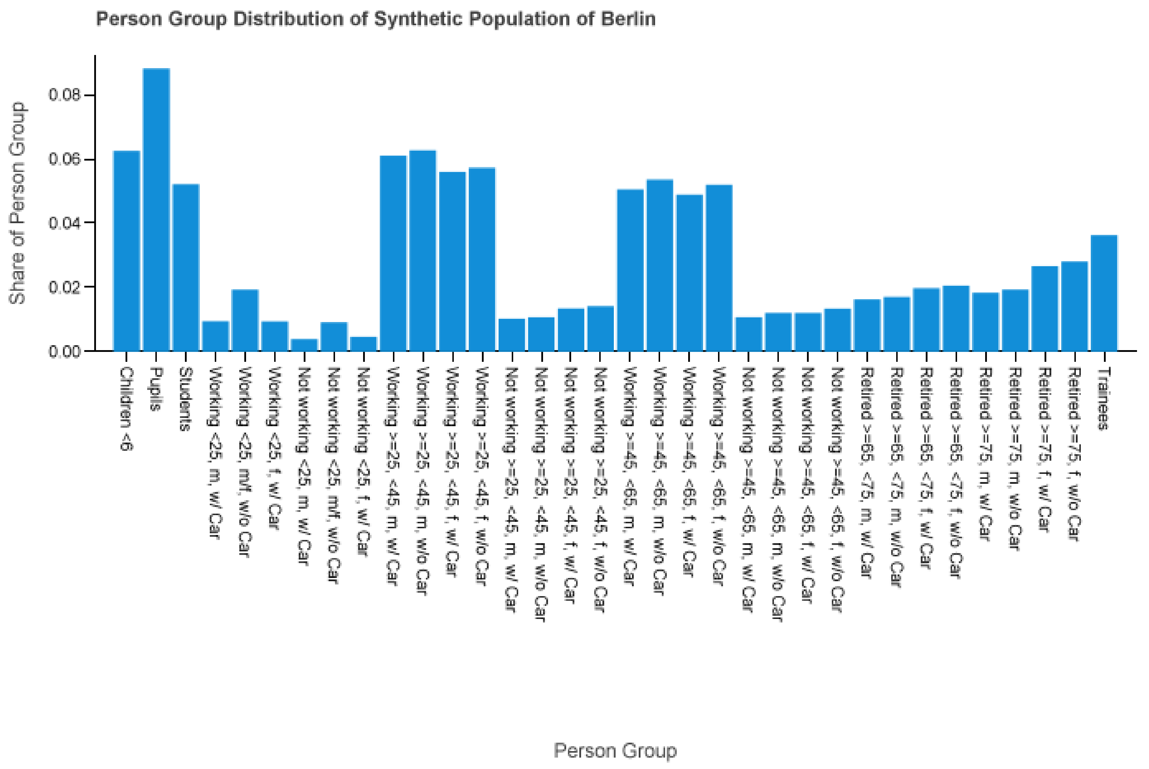
Figure 2 details the distribution of the person groups. The status like student, working or pupil defines the first split into several group segments. The numbers specify the age range, e.g., from 25 to under 45. The sex is stated by male or female. For groups where the gender is not of importance we write m/f or omit it entirely. “W/(o) car” indicates the car ownership. Sex, age, and car attributes are omitted if it is not of significance for the person group, like pupils, students, and trainees. We decided on this group division by analyzing the available input data and forming homogeneous user groups of interest. The age classes are chosen to reflect certain periods of life, like first job (<25), young professionals (25–45), senior professionals (45–65), young retirees (65–75) and old retirees (>75). Doing so we had to meet two external constraints: The group size must not drop to less than 100 diaries. Separation between male and female is only necessary, if the frequency of activities in their diaries differ more than 1%.

Figure 2.
Person group distribution of a synthetic population of Berlin.
One can immediately see the smaller share of unemployed people or the higher share of retired women compared to men. The attributes from Section 2.1 are used to classify a person to a person group like students or working women between 45 and (excluding) 65 without a car. Therefore (as seen as in Table 2), each diary d is assigned to a person group. We write or only if it is obvious to which diary it refers to or if the diary is not of importance. For the weighting we considered two diary filters:
- Diaries of all regions from Monday to Sunday; and
- Diaries from regions with more than 0.5 M inhabitants during core weekdays (Tuesday to Thursday) only.
Filter 1 represents an average of the whole week over all regions but with the population distribution of Berlin. This may be no realistic image but suffices for research purposes. For Filter 1, we write the set of diaries as . Filter 2 models a typical workday in a metropolitan area. This case may be transferable to other larger cities in Germany, such as Hamburg, Munich or Cologne, but further attention to the respective population is needed. For Filter 2, we write .
To adapt the diaries we gave each diary d with person group a weight depending on the filter. Because each diary within one person group and MiD set will have the same weight, we can write . The weight of a specific person group is defined as
where is the shorthand notation of the number of people in person group from the synthetic population. D is a placeholder for and , where . is the number of people in Berlin. denotes the cardinality of set X as usual.
2.3. Diary Classes and Probability Distributions
For a microscopic agent-based simulation of the activity travel behavior of a population one could be satisfied with a single division into person groups. Each person (i.e., agent) takes a reported diary of its person group. This leads to problems due to a lack of reported diaries in specific person groups. For example the person group of non-working under 25-year-olds without a car reported only 39, 32, and 56 diaries in 2002, 2008, and 2017, respectively. This further decreases if someone wants to use the diaries of metropolitan regions during the middle week days to get an image of a typical work day in bigger cities like Berlin. In this case only 3, 5, and 6 diaries are reported respectively.
Because of this, we use diary groups which assign to each diary a specific group with a special commonality between all diaries within a group. Hertkorn et al. [12,13] uses sequence alignment and clustering algorithms to classify diary groups. We use a different and simpler classification of diary groups with a more straight forward way of assigning the diaries by its activities. We discuss the uncertainties of this approach later in Section 4. Table 3 presents the diary groups we used. Note that, despite escort trips defining some diary groups we will later conflate escort trips into any activity.
Table 3.
Diary groups.
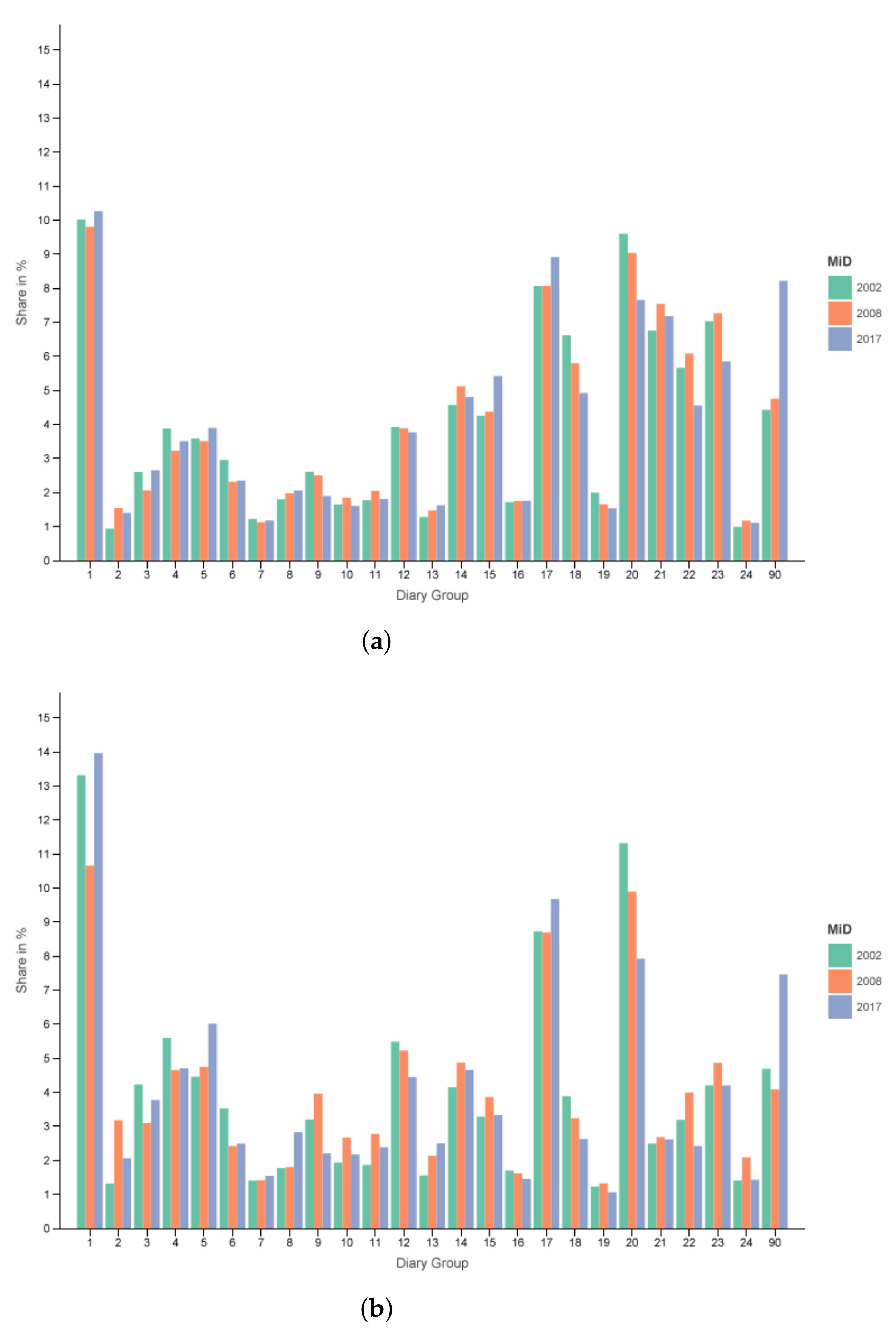
The distribution for all regions and all days can be seen in Figure 3a and for metropolitan regions from Tuesday to Thursday in Figure 3b. One can see that share of working (1–10) and educational (11–13, 24) diaries is higher for the core weekdays. Furthermore, a drastic decrease in free time diaries of persons who (usually) work (21) or go to an educational institution (22) with a smaller reduction for non-working people (23) is visible when comparing the two filters.
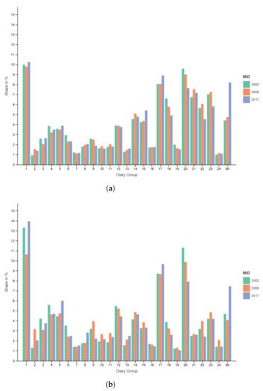
Figure 3.
Diary group distribution. (a) Dx, all Regions from Monday to Sunday. (b) Dx, cities with ≥0.5 M inhabitants from Tuesday to Thursday.
Note that, the diary groups have in our case different priorities. The highest priorities are educational diaries for specific groups like children, pupils, students and trainees. Educational trips by working or non-working people—such as going to a language class in the evening—are of lowest priority. Other than that it goes roughly in the order of its numbering. The exceptions are
- (1) which comes after (2), (3), (4), (5); and
- (6) which comes after (7), (8), (9), (10)
For example if a diary of a student is reporting a trip to the university it will belong to diary group (11) no matter if the student is going to do its students job on the same day. Another example: If an employee is not going to work on the day of the report but goes shopping and to their yoga class (free time), the diary will belong to group (18), but not (21), because (18) has the higher priority over (21).
The purpose of these diary groups is to have a greater pool of available diaries for the person groups and introduce less homogeneity. Considering the example of a student, it may be the case that the student is going to the university and, hence, diary group (11) is chosen. Nevertheless, a student may behave on a single day like a typical full time worker and doing their 8-hour shift of their students job. In case of a full-time work day the person chooses a diary of group (1)–(5) or for part-time work group (6)–(10).
This leads to a probability distribution where denotes the probability of a person in person group choosing a diary in diary group .
where D is again a placeholder for and . Furthermore, we specifically write and . It holds
where ( in our case) is the set of diary groups. For a person p of group , instead of only using the diaries belonging to the person group this approach enables us to possibly assign any diary in the diary groups with .
3. Results
3.1. MiD Data Results
To get the share for each activity we compute
where is the weight of person group of diary of trip t.
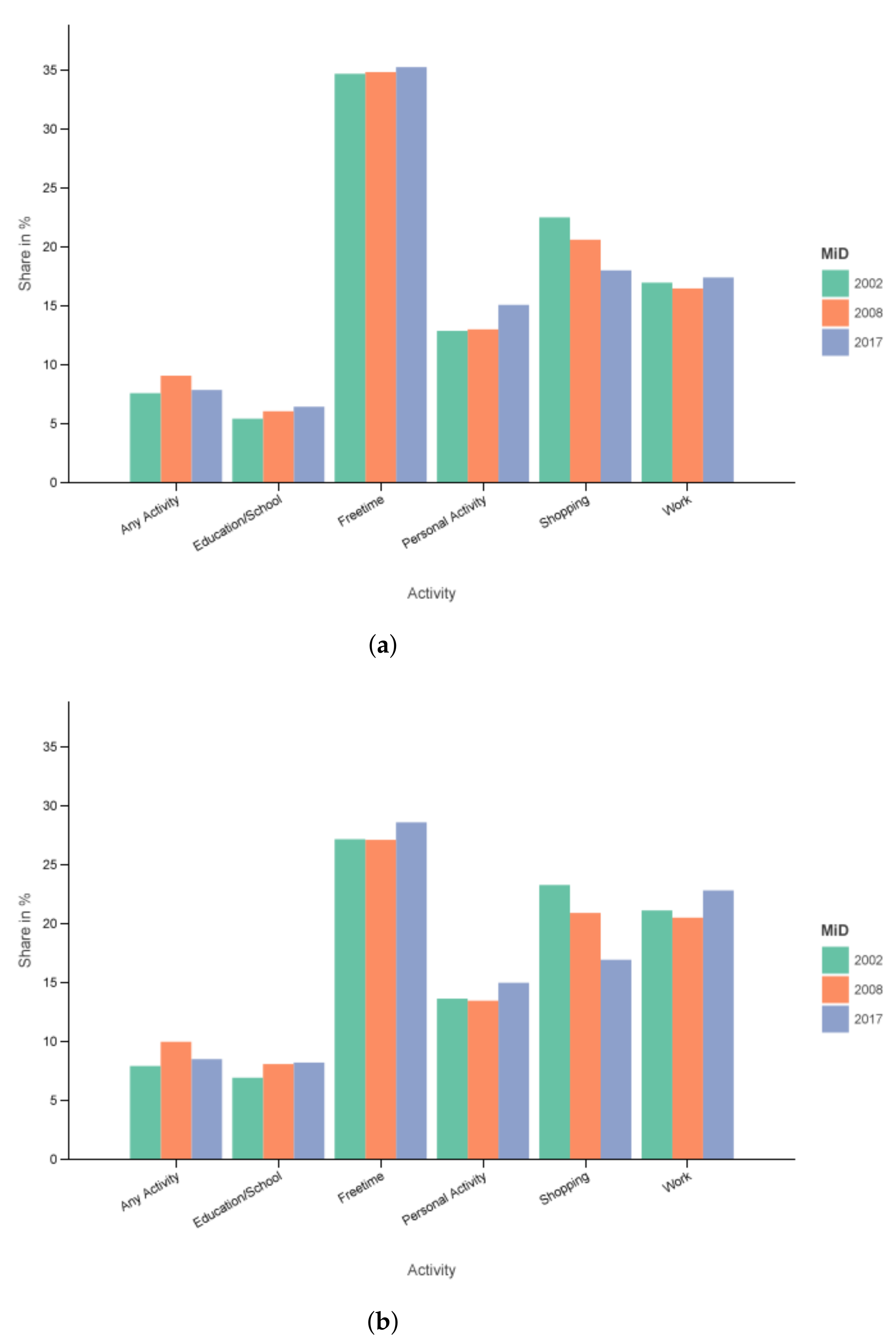
The specific values in percent for the two filter sets Filter 1 () and 2 () of can be seen in Table 4 and in Figure 4a,b.
Table 4.
Activity share of the MiD time series report for the two filters.
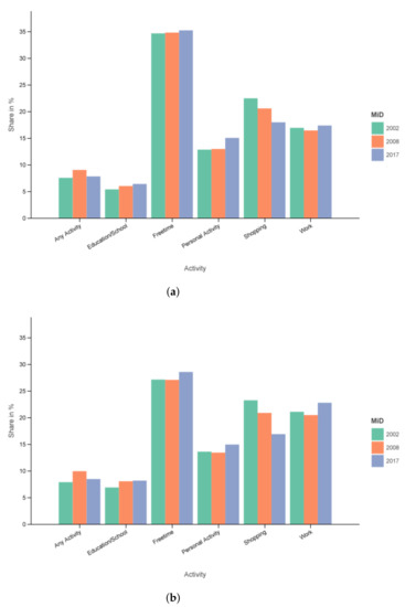
Figure 4.
Activity share in the MiD over time. (a) All regions, Monday–Sunday. (b) Cities with more than 0.5 M people, Tuesday–Thursday.
Free time has the biggest share in all cases by a good margin. Unsurprisingly, one can see a lower share of roughly eight percentage points for free time in the core weekdays in metropolitan areas. The shopping activities, especially in Figure 4b, have the biggest decrease over time. All other activities are at least in relative parts increasing from 2002 to 2017, either strictly (e.g., education) or with a bump or dent in its course (e.g., any activity, work).
3.2. Diary Class Distribution Results
When using the probability distribution from Equation (1), we compute the of each activity a for our Berlin population applied to each MiD report through
Like above, is the cardinality of the person group in the Berlin population. denotes the number of diaries in diary group with respect to . Note that, to maintain diary heterogeneity, we use the whole set of diaries of each year , respectively. In case of the diary class distributions the Filter 2 is only applied to the probability computation.
Table 5 shows the distribution of activities for each combination
of diaries and probability distributions . Comparing the MiD 2002, 2008, 2017 development of the frequencies of the activities to the entries where only the probability distributions change one can make the following observations:
Table 5.
Overview of activity percentages for each combination of diary and probability distribution. Columns where the years of diaries correspond to the probability distribution are highlighted. and are the respective filters 1 and 2.
- The development of free time and any activity is never met;
- –
- These two activities have the lowest priority according to our diary group order;
- The development of education is only achieved for all regions and all days (it rises twice from 2002 to 2017) but not for bigger cities in the core workdays (again rises twice). The probability prediction states an increase at first and a smaller decrease from 2008 to 2017;
- –
- A (half) mis-prediction despite being the highest priority group for children, pupils, students, and trainees;
- –
- The share of educational trips in diaries not in diary class (11), (12), (13), (24) are 1.28% (2002), 1.15% (2008) and 1.17% (2017) for all regions and days. Because of these diaries which can fall into any diary group the number of estimated educational trips seems always lower than the reported number from the MiD;
- –
- For bigger cities, Tuesday–Thursday we have 1.68%, 1.56% and 2.26%. This also leads to an increased error (again using all diaries but with probabilities from the filtered set), especially for the 2017 set;
- The trends of work, personal matters and shopping are reached in both cases.
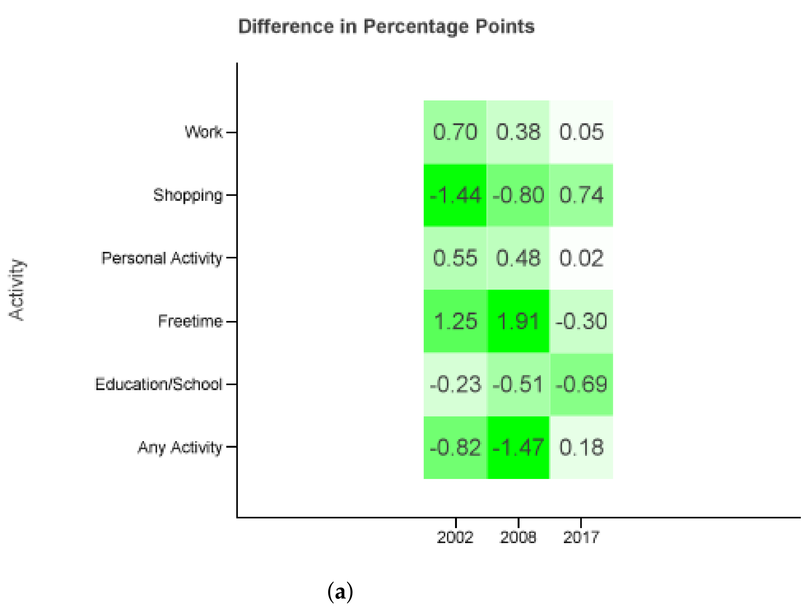
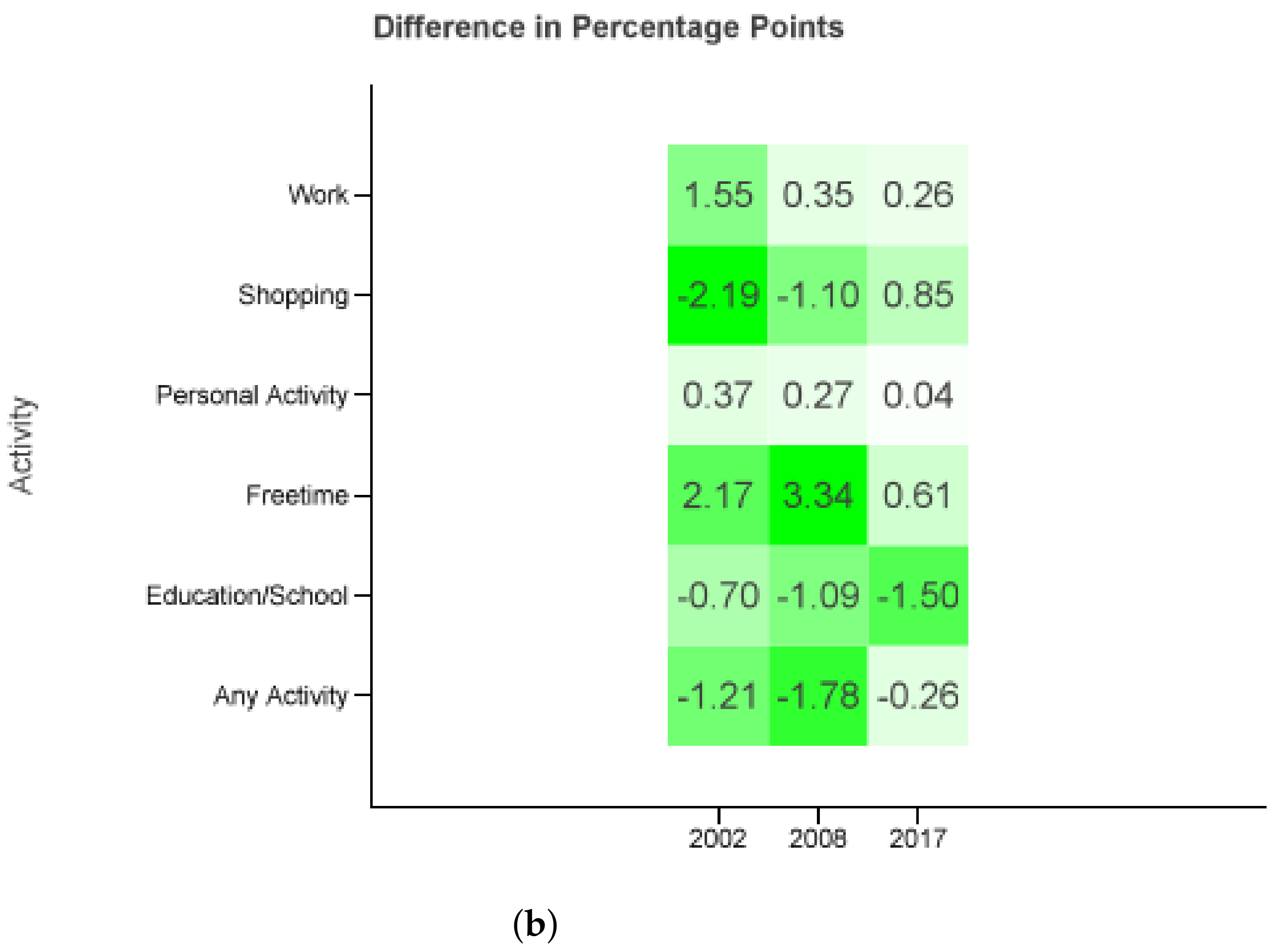
Figure 5 presents the difference between Table 4 and Table 5. In more detail, the figure shows the result of with in respect to and in regard to diaries . The same is done for Filter 2 and the corresponding sets. In the x axis, the first number corresponds to year x and the second to year y. The maximal absolute error in (2002, 2002), (2008, 2008), (2017, 2017) is below one percentage point for Filter 1 and increases to 2.58 percentage points difference for Filter 2. The bigger error for the latter one may be because of the used diaries of all regions and days which are not representative of bigger cities and core workdays. One example causing this effect might be having less free time in the core week. Especially for the columns where the year of the used diaries coincides with the year of the used probability distributions have very low differences. Considering all columns the absolute maximum error increases to 2.21 and 3.45 percentage points, respectively.
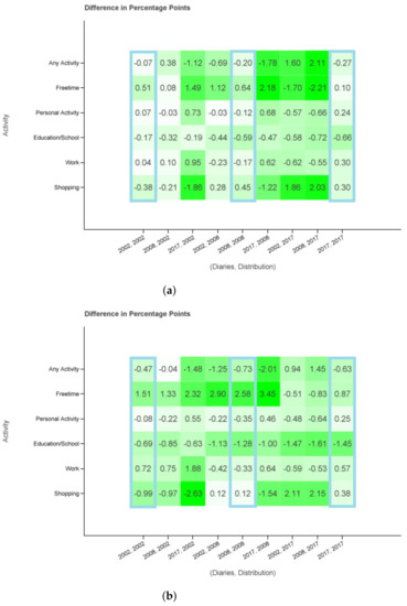
Figure 5.
Difference in percentage points. The differences are taken against the MiD values of the same year as the probability distributions. (a) All regions, Monday to Sunday (b) Cities ≥0.5 M, Tuesday to Thursday.
The absolute value of differences is particularly small for the activities education, work and personal matters regardless the combination of x and y. The absolute difference for these activities is never above 1.0 () or 2.0 () as opposed to the other three activity categories. The effect of activity priorities in building the diary groups seems to be substantial.
3.3. Union of Diaries
To further increase the available set of diaries we now use the whole MiD time series report set
The probability distributions remain unchanged and specific to a single survey year, as seen in Equation (1). The activity shares of the respective year and filter are displayed in Table 6. Looking at the development of activity behavior again one can see a similar picture compared to the data from Table 5 with personal activities, shopping, and work matching the trend, free time, and any activity failing and educational trips doing both with the corresponding filter.
Table 6.
Activity shares using the diaries of 2002, 2008 and 2017 together with the probability distributions of a single year.
The closest results delivers compared to the MiD 2017 values (see Figure Figure 6). It is only surpassed by for the same MiD from Figure 5. Given that the 2017 diary set outnumbers the sets from 2002 and 2008 drastically, and yield a less accurate outcome. Once again the projection models educational, work, and personal matter trips more accurate similar to Section 3.2.


Figure 6.
Difference in percentage points. Probability distributions of each survey combined with the whole set of diaries of the three reports (2002, 2008, 2017). The differences are taken against the MiD values of the same year as the probability distributions. (a) All regions, Monday to Sunday. (b) Cities ≥0.5 M, Tuesday to Thursday.
We see that the differences are greater than for . To verify that the increased error can be reduced by using only diaries of bigger cities from Tuesday to Thursday we consider
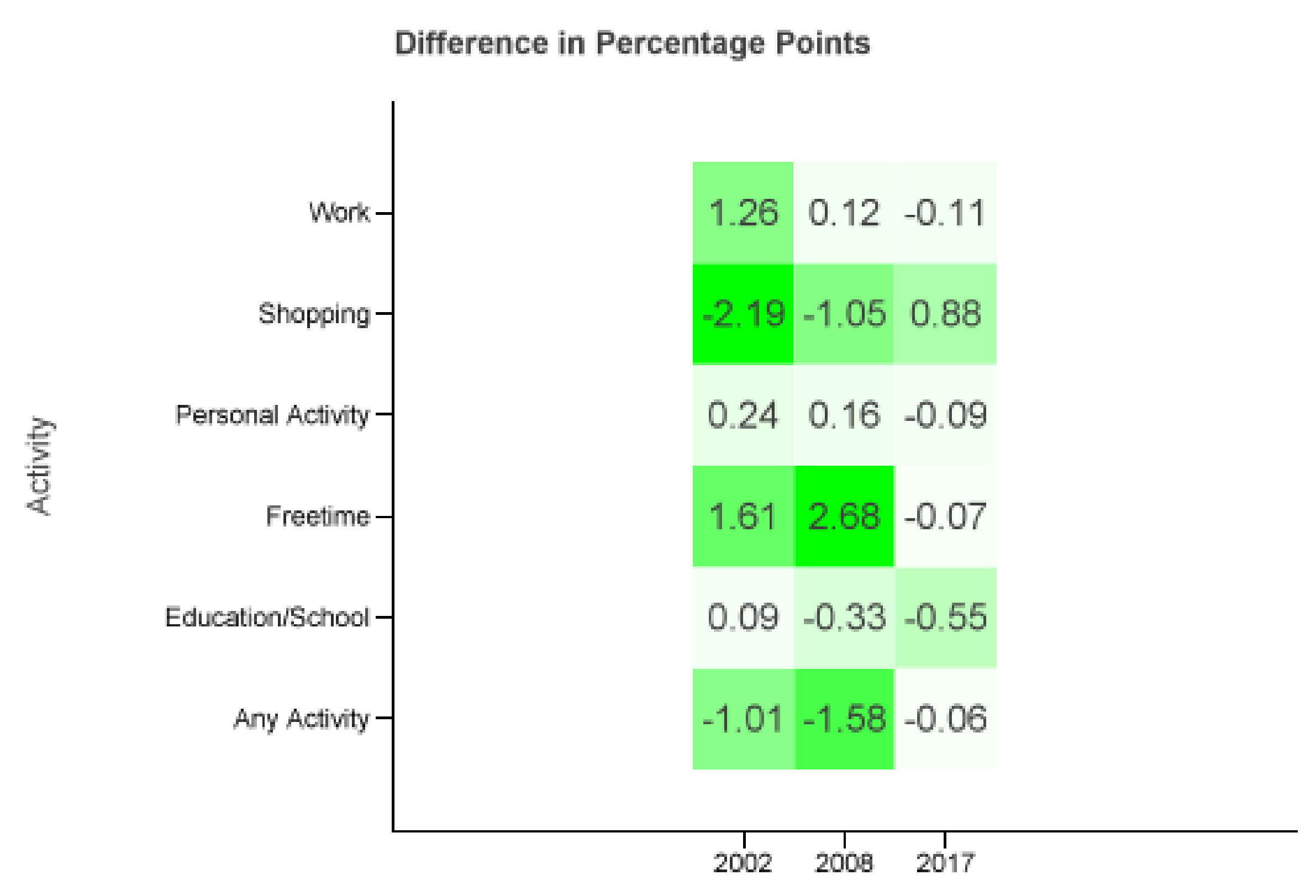
Figure 7 displays the differences of the combinations of . Comparing it to Figure b one can see that the absolute maximum error decreases from 3.34 to 2.68 percentage points. In fact, there are two cells (shopping and personal matters in 2017) with a bigger and one cell (shopping in 2002) with the same absolute difference. All other activities and years are closer to the MiD data.

Figure 7.
only using diaries from cities ≥0.5 M from Tuesday to Thursday.
The filtering of used diaries increases accuracy. There are 24,056 diaries in as opposed to 332,970 in . The question remains if there are sufficient diverse diary data for the individual use case.
4. Discussion
This paper shows a way to use probability distributions between person and diary groups which enables the use of more diaries per person group while still being fairly accurate.
Even though we did not change the population in our computation, this approach is sensitive to changes in person group distributions. A calibrated (i.e., weighted) set of diaries would still work in a new and possibly future population. An increase in, for example, pupils and students would increase the number of educational trips. With new probability distributions, possibly derived from less extensive additional mobility behavior surveys, one could use this approach and project the future activity choices based on the survey results.
Trends like online shopping, part-time or remote work had an impact on the mobility behavior in the past and is expected to have impact in the future too. However, in the past, trips which became unnecessary were not omitted but are rather replaced especially by free time activities. A change in the number and purpose of trips strongly affects mode choice and, hence, air pollution or CO2 and noise emission, especially considering trips by cars. The projection of these changes in travel behavior together with a demographic change need to be considered for developing evaluation strategies and political measures towards a sustainable mobility. A similar reasoning and its connection between the mobility behavior and the environment is explained in the DLR project report of Transport and the Environment (VEU) [21].
The findings of this work are included in the travel demand generation program TAPAS [7,8] from the Institute of Transport Research of the DLR. The first step in TAPAS is to assign activities for each person in the study area, using the probability distributions from this work. Afterwards the locations and modes of transport are chosen with respect to the personal mobility options and the spatial constraints like public transport service or access restriction for cars. Finally, the resulting diary plans are evaluated by their financial and temporal feasibility. This process is repeated until a feasible diary plan for every person is found. Doing so makes the final plan sensitive to changes in activities, locations, and modes. A full simulation output of a study area represents the decisions of the population with respect to the simulated political measures. Again, the probability distributions lead a way of modeling activity behavior. However, it is also possible that under a given activity behavior and new political measures (e.g., area restriction, gasoline price increase) the simulated outcome of chosen activities can differ from the national households surveys due to many retries in the diary plan selection. As a result we can measure if the desired sustainability goals are reached in the simulation and how the population has to adapt its activities via the presented probability distributions to the simulated scenario.
In parts future (or past), travel behavior can be projected with our model. Depending on the activity and its priority, like work and personal matters, the development is depicted accordingly in an accurate way. Other activities, such as free time, exhibit more inexact results, have outliers or show wrong trends.
The use of a more filtered dataset, such as the metropolitan regions from Tuesday to Thursday (Filter 1, ) leads to less accuracy. The quandary is to only use the diaries from the filter (not only for the probability distribution) and be more accurate versus using all diaries and have a more diverse behavior.
Problems Needing Further Investigation
One important question is, is the classification of person groups and diaries reasonable and the most accurate way? It might be the case that car ownership is of importance for the mode choice but not for the activity choice. It seems plausible that a person’s or household’s activity choices are more affected by having one or more children leading to more escort trips for instance. A deeper analysis of persons and household attributes and the resulting choices may lead to different groups. Another option would be the use of clustering algorithms, such as Hertkorn et al. [12,13] and Varschen [11] demonstrated for person groups. Nevertheless, the remaining obstacles could be the justification, the lack of comprehensibility of clustered groups, and the transferability to other mobility and household surveys.
We have seen that the priority in the assignment of diaries to the diary groups play an important role in the accuracy and quality of mimicking the trends in travel behavior. Presumably the current diary group division is not the best one possible. Especially, because none of the probability time series were capable of following the trend of free time trips despite free time contributing the largest amount of trips. A reconsidering of priorities is compelling. Hertkorn [13] and Varschen et al. [11] used sequence alignment and clustering algorithms to classify diaries into diary groups. It is not clear to what extent a general overhaul of the diary classification similar to the person groups may be necessary, but it is an interesting research topic nevertheless.
The two divisions of persons and diaries together may lead to small numbers of reports. This could cause over- or under-representation of specific behavior. Larger mobility datasets and more diaries may overcome this problem but mobility surveys are expensive. For now, it does not seem realistic to have an improvement in this data situation. One option may be the generation of synthetic diaries. Given that these are sufficiently realistic and accurate, a large number would further increase the individual heterogeneity even with or without an extra diary class distribution.
Further research in these areas are necessary in the future to improve the methodology of probability distributions in travel demand generation.
Author Contributions
Conceptualization, M.H. and A.R.; methodology, A.R. and M.H.; software, A.R.; validation, A.R. and M.H.; formal analysis, A.R.; investigation, A.R.; resources, A.R. and M.H.; data curation, A.R.; writing—original draft preparation, A.R.; writing—review and editing, M.H.; visualization, A.R.; supervision, M.H.; project administration, M.H. Both authors have read and agreed to the published version of the manuscript. All authors have read and agreed to the published version of the manuscript.
Funding
This research was funded by AutoMover and UrMo Digital of Programmdirektion Verkehr DLR grant number 2837038 and 2847012.
Institutional Review Board Statement
Not applicable.
Informed Consent Statement
Not applicable.
Data Availability Statement
Restrictions apply to the availability of the analyzed data. Data was obtained from the Bundesministerium für Verkehr und digitale Infrastruktur (BVMI) and are available at https://www.dlr.de/cs/desktopdefault.aspx/tabid-699/ (accessed on 9 August 2021) after request.
Conflicts of Interest
The authors declare no conflict of interest.
Abbreviations
The following abbreviations are used in this manuscript:
| MiD | Mobilität in Deutschland (Mobility in Germany) survey |
| d | Diary |
| Diaries of all regions and all weekdays of year x | |
| Diaries of regions with more than 0.5 M inhabitants from Tuesday | |
| to Thursday of year x | |
| Diary group | |
| Person group | |
| Set of all diary groups | |
| Set of all person groups | |
| Probability distribution with respect to diaries | |
| Probability distribution with respect to diaries | |
| Number of elements in set X. |
References
- Umweltbundesamt 2021, Treibhausgasemissionen: Emissionsquellen. Available online: https://www.umweltbundesamt.de/themen/klima-energie/treibhausgas-emissionen/emissionsquellen#energie-stationar (accessed on 9 August 2021).
- Höltl, A.; Heinrichs, M.; Macharis, C. Analysis of rebound effects resulting from improved vehicle efficiency applied to the Berlin city network. In Sustainable Urban Transport; Attard, M., Shiftan, Y., Eds.; Emerald Group Publishing: Bingley, UK, 2014; Volume 7, pp. 229–249. ISBN 978-1-78441-616-4. [Google Scholar]
- Institut für Angewandte Sozialwissenschaft (infas); Deutsches Institut für Wirtschaftsforschung (DIW). Mobilität in Deutschland 2002—Ergebnisbericht, Studie von infas, DIW im Auftrag des Bundesministeriums für Verkehr und Digitale Infrastruktur. Available online: http://www.mobilitaet-in-deutschland.de/pdf/ergebnisbericht_mid_ende_144_punkte.pdf (accessed on 11 August 2021).
- Institut für Angewandte Sozialwissenschaft (infas); Deutsches Zentrum für Luft- und Raumfahrt (DLR). Mobilität in Deutschland—MiD 2008 Ergebnisbericht, Studie von infas und DLR im Auftrag des Bundesministeriums für Verkehr und Digitale Infrastruktur. Available online: http://www.mobilitaet-in-deutschland.de/pdf/MiD2008_Abschlussbericht_I.pdf (accessed on 11 August 2021).
- Nobis, C.; Kuhnimhof, T. Mobilität in Deutschland—MiD 2017 Ergebnisbericht, Studie von infas, DLR, IVT und infas 360 im Auftrag des Bundesministeriums für Verkehr und Digitale Infrastruktur. Available online: http://www.mobilitaet-in-deutschland.de/pdf/MiD2017_Ergebnisbericht.pdf (accessed on 11 August 2021).
- Nobis, C.; Kuhnimhof, T.; Follmer, R.; Bäumer, M. Mobilität in Deutschland—Zeitreihenbericht 2002–2008–2017, Studie von infas, DLR, IVT und infas 360 im Auftrag des Bundesministeriums für Verkehr und Digitale Infrastruktur. 2019. Available online: http://www.mobilitaet-in-deutschland.de/pdf/MiD2017_Zeitreihenbericht_2002_2008_2017.pdf (accessed on 11 August 2021).
- DLR Institute of Transport Research, TAPAS Webpage. Available online: https://www.dlr.de/vf/desktopdefault.aspx/tabid-12751/22270_read-29381/ (accessed on 11 August 2021).
- DLR Institute of Transport Research, TAPAS Source Code. Available online: https://github.com/DLR-VF/TAPAS (accessed on 11 August 2021).
- Heinrichs, M.; Krajzewicz, D.; Cyganski, R.; von Schmidt, A. Introduction of car sharing into existing car fleets in microscopic travel demand modelling. Pers. Ubiquitous Comput. 2017, 21, 1–11. [Google Scholar] [CrossRef]
- Justen, A.; Cyganski, R. Decision-making by microscopic demand modeling: A case study. In Proceedings of the Transportation Decision Making: Issues, Tools, Models and Case Studies, Venice, Italy, 13–14 November 2008. [Google Scholar]
- Varschen, C.; Wagner, P. Mikroskopische Modellierung der Personenverkehrsnachfrage auf Basis von Zeitverwendungstagebüchern. In Proceedings of the 7th Aachener Kolloqium “Mobilität und Stadt” (AMUS), Aachen, Germany, 7–8 September 2006; pp. 63–69. [Google Scholar]
- Hertkorn, G.; Kracht, M. Analysis of large scale time use survey with respect to travel demand and regional aspects. In Proceedings of the International Association for Time Use Research Conference (IATUR), Lisbon, Portugal, 15–18 October 2002. [Google Scholar]
- Hertkorn, G. Mikroskopische Modellierung von Zeitabhängiger Verkehrsnachfrage und von Verkehrsflußmustern, Dissertation. Available online: https://elib.dlr.de/21014/ (accessed on 11 August 2021).
- von Schmidt, A.; Cyganski, R.; Krajzewicz, D. Generierung synthetischer Bevölkerungen für Verkehrsnachfragemodelle, ein Methodenvergleich am Beispiel von Berlin. In Proceedings of the Optimierung in Verkehr und Transport (HEUREKA’17), Stuttgart, Germany, 22–23 March 2017; pp. 193–210. [Google Scholar]
- Statistisches Bundeamt, Mikrozensus 2015. Available online: https://www.destatis.de/DE/Methoden/Qualitaet/Qualitaetsberichte/Bevoelkerung/mikrozensus-2015.pdf;jsessionid=FE082318CCACFC78C8A0F48C95C0ED88.live712?__blob=publicationFile (accessed on 13 June 2021).
- Senatsverwaltung für Bildung, Jugend und Familie, Zahlen Daten Fakten—Berufliche Schulen. 2018. Available online: https://www.berlin.de/sen/bildung/schule/bildungsstatistik/zahlen_daten_fakten_bs_2017_18.pdf (accessed on 8 September 2021).
- Nexiga, Marktdaten—Demographie. Available online: https://www.nexiga.com/datensuche/marktdaten-demographie/ (accessed on 13 June 2021).
- Nexiga, Marktdaten—Haushalte. Available online: https://www.nexiga.com/datensuche/marktdaten-haushalte/ (accessed on 13 June 2021).
- Deutsche Rentenversicherung, Rentenatlas 2018. Available online: https://www.deutsche-rentenversicherung.de/DRV/DE/Experten/Zahlen-und-Fakten/Statistiken-und-Berichte/statistiken_und_berichte.html (accessed on 13 June 2021).
- Amt für Statistik Berlin-Brandenburg, Statistisches Jahrbuch 2018. Available online: https://www.statistik-berlin-brandenburg.de/produkte/Jahrbuch/jb2018/JB_2018_BE.pdf, (accessed on 13 June 2021).
- Henning, A.; Plohr, M.; Özdemir, D.; Hepting, M.; Keimel, H.; Sanok, S.; Sausen, R.; Pregger, T.; Seum, S.; Heinrichs, M.; et al. The DLR Transport and the Environment Project—Building competency for a sustainable mobility future. In Proceedings of the 4th Conference on Transport, Atmosphere and Climate, Bad Kohlgrub, Germany, 22–25 June 2015. [Google Scholar]


Publisher’s Note: MDPI stays neutral with regard to jurisdictional claims in published maps and institutional affiliations. |
© 2021 by the authors. Licensee MDPI, Basel, Switzerland. This article is an open access article distributed under the terms and conditions of the Creative Commons Attribution (CC BY) license (https://creativecommons.org/licenses/by/4.0/).