Built Environment Characteristics, Daily Travel, and Biometric Readings: Creation of an Experimental Tool Based on a Smartwatch Platform

Abstract

Travel surveys can uncover information regarding travel behaviour, needs, and more. Collected information is utilised to make choices when reorganising or planning built environments. Over the years, methods for conducting travel surveys have changed from interviews and forms to automated travel diaries in order to monitor trips made by travellers. With the fast progression of technological advancements, new possibilities for operationalising such travel diaries can be implemented, changing from utilising mobile to wearable devices. Wearable devices are often equipped with sensors which collect continuous biometric data from sources that are not reachable from standard mobile devices. Data collected through wearable devices range from heart rate and blood pressure to temperature and perspiration. This advancement opens new possible layers of information in the collection of travel data. Such biometric data can be used to derive psychophysiological conditions related to cognitive load, which can uncover in-depth knowledge regarding stress and emotions. This paper aims to explore the possibilities of data analysis on the data collected through a software combining travel survey data, such as position and time, with heartrate, to gain knowledge of the implications of such data. The knowledge about the implications of spatial configurations can be used to create more accessible environments.

1. Introduction

Travel surveys have been used for decades to observe patterns, locations, and choices made by travellers, in an attempt to understand their needs and behaviour [1,2]. By utilising this information, it is possible to make strategic planning decisions and monitor the realisations of such decisions. As we are striving for an equal society, it is crucial to understand why and how inhabitants are affected by their surroundings to create more accessible areas. There are currently several ways of conducting travel surveys, including traditional pen and paper surveys [1], interviews, and semi-automated collection methods utilising mobile technologies to create travel diaries for travellers [3,4,5,6,7]. As we strive to acquire more reliable and trustworthy data, these methods that are close to automatic data collection are developed to use machine learning methods to predict, analyse, and label the collected data. The progression has been rapid, and it is now possible to not only collect the data about where the traveller is travelling but also to predict or conclude the chosen travel mode using a fusion of several sensors such as gyroscopes and accelerometers [8]. This progression in methodologies to collect data makes it possible for the survey participant to travel as usual, and then one can review their collected data afterwards. This gives the possibility to either acknowledge and approve the collected data or change it where there might be incorrect data. These methods will more independently collect the data the further they are developed

However, the trend of utilising more data sources to predict additional data, such as accelerometer and gyroscope data, which predict travel modes utilising machine learning methods, open the possibility to collect additional biometric data from the survey participant. With the currently available technology, it is not only possible but also easy to obtain biometric data such as heart rate using wearable devices that resemble watches [9,10,11,12,13,14,15,16,17,18]. By adding the collection of such biometric data, it is possible to extract more information that might relate to psychophysiological conditions, such as cognitive load and stress, from biometric sensors [19,20,21,22,23,24,25]. The addition of the possibility of deriving such information opens a new perspective on how travel surveys can be enriched, analysed, and deployed.

To explore this new field, we have been experimenting with and designing a method which combines biometric data and traditional travel information related to positioning, and the software that implements this is currently in the development stage [26,27]. This method in development has previously been tested, and it has been demonstrated that it is possible to collect the required data. This new data collection method with the developed software opens the possibility of analysing the additional data collected and to see what type of information can be derived from it.

This paper will cover the data analysis of a data set collected through the use of a proof-of-concept stage software in order to uncover how travellers are affected by the built environment, by comparing biometric data deviations at specific locations and data which have been collected automatically using positioning and biometric sensors in combination.

The outline of the paper is, first, the background section that aims to cover related work and how the result could relate to this paper’s conclusion. The methodology will be divided into two parts; (1) the first part covers how and what data are collected and the processes revolving around the collection of the data set for this particular paper; (2) the second part covers analysis methods explored in the process of analysing data sets. The results will be presented in the section following the methodology, and a discussion evaluates the results based on the recent work presented in the background. Finally, the conclusion section will conclude the experiment and point out key findings from work presented in the paper, focusing on the implications of utilising biometric data as a feature for travel surveys, the result of which is aimed at urban and transport planners in general.

2. Background

This section aims to cover related articles and reports to create a background for the paper. The chosen references are related to the collection and analysis of data through mobile and wearable devices to show the possibilities that the recent discoveries have granted the research fields of transport planning, as well as geoinformatics and urban planning.

2.1. Data Collection

To create a background for the intended analysis methods in this paper, this section aims to explain how travel diaries function and what biometric data could be added to enrich the result of the analysed data. For more information on how these ubiquitous datasets, in general, can be used to analyse and model travel choices and behaviours, please see Chen et al. [2], Li et al. [28], and Rashidi et al. [29] for examples.

2.1.1. Collection of Biometric Data

Recent technological advancement has led to the development of biometric sensors being implemented in consumer-grade hardware [9,10,11,12,13,14]. This development means that biometric data become available in even more substantial quantities than before, since it is possible to create software implementing biometric data collection for widely available platforms, such as Android Wear [30] and watchOS [31]. Much like automated travel diaries for mobile phones, software for these widely available platforms makes it possible to reach device users in a more effective manner than before, since it requires less activity from both the device user to participate and for the researcher to distribute software and hardware, as the user can utilise their own hardware and the researcher can distribute their software through operating system dependant marketplaces [32,33]. Recent research shows proof that it is possible to deduce mental conditions, such as cognitive load, through the use of such types of hardware [19]. By combining several sensors, the different data streams can be used to confirm and imply these conditions. Modern consumer-grade hardware in the form of wearables often includes several types of sensors to deduce the activities of the user [15,34,35]. Such sensors include, but are not limited to, accelerometers and gyroscopic sensors (from here on referred to as “motion sensors”) for motion detection, ECG and/or PPG sensors (from here on referred to as “biometric sensors”) for heart rate and/or blood pressure, as well as GPS and GLONASS (from here on referred to as “position sensors”) for positioning [3,8,36,37,38,39,40,41,42]. The motion sensors collect information about how the device is put in motion, which then can translate to the deduction of several activities such as walking, running, climbing stairs, and more [15,34]. This information in combination with the biometric sensors, which often collect heart rate, can help in confirming those activities by comparing the level of activity with the current heart rate [18]. These sensors can also be used in combination with positioning sensors for popular activity tracking apps in order to analyse and collect data about progress, display maps over past activities, and more [43].

2.1.2. Automated Travel Diaries

Automated travel diaries are an efficient way to collect data for the analysis of travel behaviour and needs of travellers in urban areas [4]. The development of such diaries is striving to become as automated as possible, both when it comes to the collection of trip legs, but also regarding mode selection. Much like the activity applications described in the last paragraph, the travel diaries can utilise motion sensors in combination with positioning sensors to deduct travel modes, as each mode has a difference in the movement signature [44,45,46,47]. This type of deduction is performed by comparing previous data with the new input to find the most likely answer to the question of mode choice. With the same methodology, it is possible to find deviations in the movement patterns. Traditional travel diaries that are often entirely manual incorporate the recording of such factors as well as metadata to understand the reason for traveling to the destination, etc. [1]. For example, Prelipcean et al. [48,49,50] and Wang et al. [51] have provided inventories of various operational travel diary tools that have been deployed until recently. For a summary of issues that still need to be further developed to create fully automated travel diaries, refer to Prelipcean and Yamamoto [52], Gadziński [53], Stopher et al. [54], and Wang et al. [51].

The related work presented in 2.1 has shown the possibilities of collecting a wide range of data types through simple means available to the public, and it is therefore possible for researchers to use, in large quantity, data collections. The next section will describe how the collected data can be analysed through different data-driven methods.

2.2. Analysis Methods

Machine learning has been a relevant topic in the field of data analysis for years [55]. It simplifies the process of applying statistical methods to data sets to capture relevant results. Instead of programming complex rulesets for each specific data set, machine learning provides the possibility to reuse more general algorithms for many data sets, without having to program for specific scenarios. There are many methods to choose from, and just as in traditional statistics, the different methods will uncover different results, depending on what has been explored. In this subsection, clustering and regression methods will be described and compared as a basis for the methodology of the data analysis in this paper.

2.2.1. Partition Clustering

As the focus of this paper is to analyse biometric and positioning data to find how areas and locations might affect travellers, a strategy called partition clustering can be used to find out if areas within the data set are affecting the participant. Partition clustering is a general method which uses all dimensions of the data set to find patterns within which the samples can be organised.

A common partition clustering method is called “K-means clustering”, which uses all the dimensions of the data set in order to find the “distance” between each data point and the K number of reference points, taking all dimensions into consideration [56]. The reference points are at first placed at relatively random positions in which their distance to the data points is measured, and they are then moved between each run of the algorithm until they are placed in such a position in which they are the closest to “their” cluster of data, as can be seen in Figure 1. This type of clustering method is useful when one is trying to find which data points are related to each other and which are not, without any prior knowledge of the data set. When the method has compared the distances and moved the reference points to locations from which they are no longer possible to move to a more optimal position, the analysis is done, and the points of data are divided according to which reference point they are closest to. The formula of k-means clustering used is as follows, where J is the objective function, k is the number of clusters, n is the number of cases, x is the current case i, and c is the centroid for cluster j:

$$J={{\displaystyle \sum }}_{j=1}^k{{\displaystyle \sum }}_{i=1}^n{\parallel x}_i^{\left(j\right)}-c_j{\parallel }^2$$

(1)

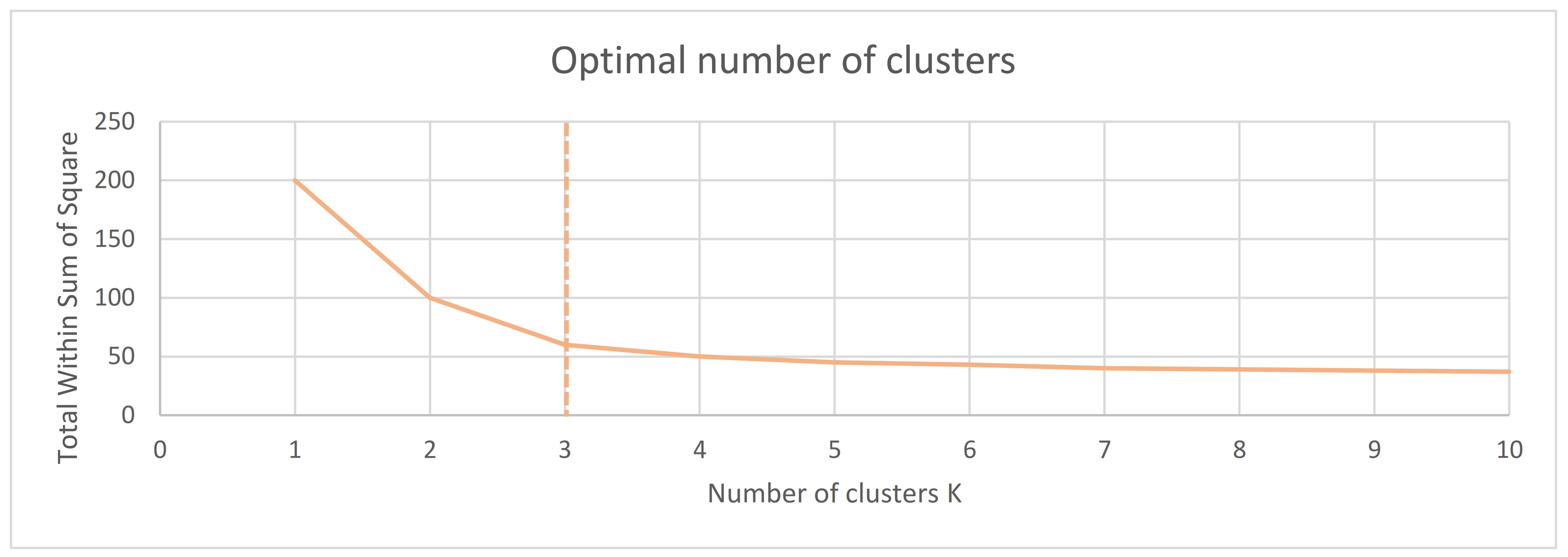
In order to find K, there are several methods to analyse the data set [57]. One example is the “elbow method”, where one runs K-means clustering on the data set iteratively with the integer K changing incrementally after each final round between two values, for example, 1 to 10. For each K, one calculates the sum of squared errors (SSE) and projects the result on a graph, with the value of K as the X-axis and the SSE as the Y-axis. At one point, an apparent elbow in the line should be visible, as can be seen in Figure 2, indicating that the K value of that point is the optimal K for the K-means clustering.

However, the elbow method can sometimes be ambiguous, as it might be hard to distinguish at what value of K the elbow is. A less ambiguous method is the Average Silhouette Evaluation (ASE) method. The algorithm is similar to that of the elbow method but deviates in the sense that, instead of calculating the SSE of each value K, it measures the quality of the clustering by iterating and finding the optimal K when the average silhouette is maximised within the set range of possible K [58].

K-means clustering is a versatile algorithm as it is unsupervised and therefore can work directly with the intended data set. It also accounts for each dimension equally, meaning that it does not put extra weight on certain features, such as position or time. However, this can be a drawback when working with spatial data, such as those described in this paper. Therefore, other methods will be described in the following paragraphs.

2.2.2. Spatial-Based Clustering

When working with spatial data, it might be beneficial to emphasize the spatial dimension of the data. There are several methods to cluster data with regards to spatial dimensions, such as density, spatial restrictions, and time intervals. As the focus of this paper is to find enclosed areas which can be compared, a suitable method for clustering the data is density-based clustering. Focusing on the spatial density of collected data will output clusters where large amounts of data have been collected in an enclosed area. These areas could then be further analysed regarding biometric data to uncover where and how travellers are affected within that area. By comparing similar areas with similar effects using data-driven methods, it should be possible to find patterns among said areas related to the specific spatial configurations and features of those locations.

Density-based spatial clustering of applications with noise (DBSCAN) can be used to cluster density-based spatial data and filter out outliers within the data set as noise [59]. Instead of using reference points with a dynamic radius to find a mean between data points, as K-means clustering does, DBSCAN utilises a set maximum radius and minimum point density. The algorithm is applied to each data point to measure how many other data points are located within the maximum radius of the point. If more than the minimum number of points is located within the radius, that point is labelled as a core point which belongs to a cluster. If less than the minimum number of points is within the radius, but at least one point within the radius is a core point, that point is a border point, which means that the analysed point is located at the border of, and belongs to, the cluster. If no points are found within the radius, or none of the found points are core points, the analysed point is an outlier and is considered as noise. A visualisation of this can be seen in Figure 3.

As with the K-means clustering, DBSCAN needs some variables to function. In K-means clustering, the number of clusters needs to be defined; however, in DBSCAN, the minimum number of points and maximum radius needs to be defined. This can be done using the elbow method, which is less ambiguous for DBSCAN as it can use decimal values rather than integers, which K-means clustering requires. An example of this can be seen in Figure 4.

This method is more efficient than K-means clustering in the sense that it can cluster data in asymmetric forms, in comparison to K-means clustering which creates a radius from the reference point in which all cluster points need to be located. It also allows for outliers to be considered as noise, as opposed to K-means clustering, which uses all data points, no matter if they are outliers or not. However, it does not uncover anything related to correlation, as it only clusters the data for further analysis. To understand how the collected data correlates, other methods will have to be used, which are described in the following section.

2.2.3. Regression

The previous sections have presented and described clustering methods which do not put emphasis or weight on any specific dimension (K-means clustering) or only focus on positioning dimensions (DBSCAN). These methods are applicable for finding patterns in the data to group a dataset into several clusters, however, there is no information regarding the correlation between dimensions that can be found using these methods. Further, there are other methods that can compare dimensions to find the correlation between them.

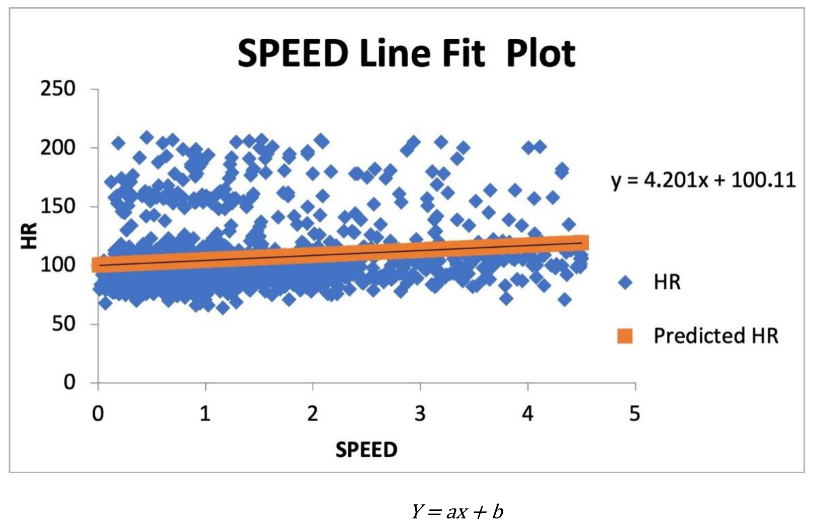
One method for comparing data and finding patterns is regression analysis. The main difference between clustering and regression is that, instead of finding a mean or a density-based body, the output of a regression analysis is the variable for an equation describing the correlation between the data dimensions that are being compared [60,61,62,63]. The simplest form of regression is called linear regression, in which the goal is to find the variables for a line that aligns with the trend of the comparisons between the data dimensions. One of the dimensions is dependent on the other, which can be described with the equation found in Figure 5.

In this equation, $Y$ is the variable that depends on $X,$ and the aim of utilising the linear regression is to find the constant $b$ and the regression coefficient $a$. When the constant and regression coefficient have been found, the equation can be used to (1) find the probability that there is a correlation between the dependent and the independent variable, or (2) predict $Y$ based on $X$. This opens the possibility of predicting dependent variables based on independent data. This prediction is useful when analysing travel behaviour and travel needs, as it can uncover a general understanding of how a particular factor in travelling is affecting the travellers. There are many types of regression analysis that can be formed, however, for the sake of the work proposed in this paper, only linear and multivariate regression will be covered. Next, the method section will explain how the data set was collected, how the data was refined, and how it was analysed.

2.3. Summary of Background

This section has covered the state of the art of biometric data collection and travel diaries, as well as methods for analysing large quantities of data. By combining the methods for collecting biometric data with the methods for automated travel diaries, the authors aim to create a new method which will uncover mental health-related effects of different areas. The analysis methods describe how large quantities of data can be restructured to show implications of how and where these health effects occur. The next section will cover how these methods will be used in this experiment.

3. Materials and Methods

Based on the background in the previous section, this section aims to explain how the data for the analysis have been collected and what methods for data collection have been used with arguments for why. As mentioned in the introduction, this paper covers the experimental analysis of a data collection tool, developed by the first author, called MERGEN [26]. The trial in this paper covers the collection of data from a small set of participants and emphasises the method to analyse the data, and what the collected data could reveal about a traveller. This is the first step in a series of experiments to uncover the possibilities of combining and collecting position and biometric data using the tool.

3.1. Data Collection

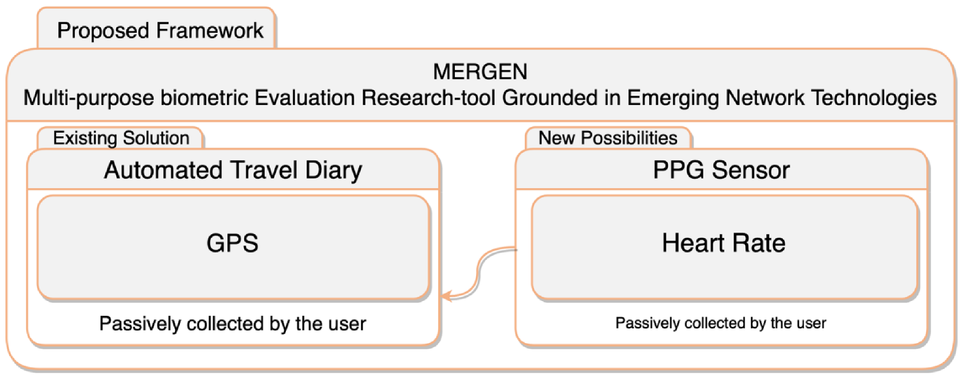
The framework for data collection used in this trial is called MERGEN and was designed based on previously available semi-automated methods of travel data collection, such as those described in Section 1 and Section 2, augmented with the addition of biometric data. The framework can be used with a range of devices; however, the version used in this trial is a software, based on a wearable specific version of Android, called Wear OS, and utilises consumer-grade hardware, such as smartwatches, which includes biometric sensors. In this case, a smartwatch with a PPG sensor designed for the collection of heart rate was used. The framework combines the collection of position data and adds the dimension of heart rate to the collected data set, as visualised in Figure 6.

The software is intended to work with any Wear OS-compatible device and is therefore designed to utilise the built-in functions for the collection of position and biometric data. This opens the possibility of choosing among a wide range of devices, with several variations of combinations of sensors. As the software had been developed and tested with the use of a Huawei Watch 2 4G, the same model of the smartwatch was used in this trial, so as to not add any additional factors which could disturb the outcome. The reason as to why this specific watch was used in the development process was because of the versatile range of sensors, shown in

Table 1. The technological specifications of the utilised hardware.

Specifications	Descriptions
Operating System	Wear OS 2
Sensors	PPG, GPS + Glonass, 6-axis A + G Sensor, 3-axis Compass, Barometer, Capacitive Sensor, Light Sensor
Communication	4G LTE, BLE, NFC (RFID), UMTS, TD-SCDMA, GSM
Screen	1,2-inch Circular AMOLED with 326 PPI
Battery	410 mAh

.

The software was tested using members of the research team as participants to gain data for analysis that were used to uncover the possibilities of a larger scale study at a later stage and to uncover what type of results that can be found using such a framework. Before the trial, all watches that were used were booted with a clean installation of the latest version of MERGEN. This means that all settings had been set to the same and it was not possible for them to be changed by the participants in the trial. The sample rate was set to be based on time rather than location, as the emphasis in this trial was on the biometric data rather than the position. This means that several data points might be collected in the same position if the person is static. This is preferable over the option of having a location-based collection which would collect a data point every X meters, as the result of heart rate changing at the same location might be of interest when searching for external factors affecting travellers and would be lost if data were only to be collected every X meters. It was also possible to set the quality of the data collected. The software was set to collect fine location data, when possible, and coarse data when fine location data was not available, due to reception differences between locations. The sample rate of the collection for all factors was set to one sample per minute, as this would interfere as little as possible with the battery life of the device, based on benchmarks made by the developers of the framework.

3.2. Data Analysis

In the previous subsection, the method for data collection was described. This subsection aims to explain what types of data analysis methods were explored and how the results were extracted and compared. The goal of the analysis was to uncover areas where the heart rate deviates from its regular patterns. The hypothesis was that it would be possible to uncover how travellers are affected by certain areas through the combined utilisation of several data analysis methods. The methods used for the analysis are described in this section and provide a background for the results, which will be presented in the following section.

The data were refined using Microsoft Excel, and all cluster-based analysis methods were explored using MATLAB R2019a with the “Statistics and Machine Learning Toolbox” as well as the “Mapping Toolbox”. The regression-based analysis was performed using SPSS 26. The analysis was conducted in a linear fashion, where each step either led to the refinement of the input data for the next step or the results for comparison between the methods. Each step will be described in-depth in the following paragraphs.

3.2.1. Data Refinement

The data were limited to a border containing location points within and around the Stockholm area in Sweden. As to not affect the comparison between different persons’ patterns, the heart rate was normalised between 0 and 1. No further data refinement was performed before the analysis.

3.2.2. K-Means Clustering

The data analysis was first explored using K-means clustering to find groupings of areas where the biometric data, in this case, heart rate, were deviating from the regular pattern. After considering the findings from the literature review, it was decided that the Average Silhouette Evaluation (ASE) method was going to be used to determine K, rather than the common elbow method, as the elbow method can be considered more ambiguous than the ASE method since it can sometimes be troublesome to choose between two integers, leading to a suboptimal K.

However, the K-means clustering does not put any weight on any of the dimensions and therefore compares all data points with the same weight per dimension. As the heart rate has a smaller range of possible values than the position, the clustering tended to organise the data according to the spatial positions rather than the locations. For this reason, the ASE method was used solely on the heart rate dimension to find the appropriate number of clusters.

Once K was defined, the data were clustered using all dimensions and K-means clustering.

3.2.3. DBSCAN

The K-means clustering organised the data into levels of heart rate deviation and unveiled where deviations in heart rate could be observed. However, to find more significant areas where travellers where affected, a clustering of locations also had to be done. To do so, a method for clustering the data regarding positioning was used. In this case, DBSCAN was decided to be suitable as it would also filter out noise points which were of no interest when comparing larger areas.

The clusters from the K-means clustering were used to create the density-based clusters. Each cluster was utilised as input in DBSCAN and the output where several areas per cluster that could be singled out and used for future comparison. However, the clusters did not implicate any information about the correlations between different factors. Therefore, linear regression was used to analyse the data and uncover if there was any correlation between the condition of the person and the specific areas.

3.2.4. Creating the Personal Biometric Model

The exploration of the data shows that there seems to be some spatial effect on the biometric data of the participant. To further analyse and understand how individual components affect the collected biometric data, a model had to be created and tested. To create the model, a comparison of the collected variables and prominent factors that could affect heart rate was performed which led to the creation of an array of variables that should be included in the model. The variables included spatial, temporal, biometric, and movement data which could be divided into the linear and categorical features that can be seen in

Table 2. The variables for the model.

Input	Derived Variables
PPG Sensor (Heart Rate Sensor)	Heart rate (linear)
GPS/GLONASS	Speed (linear)
	Points of Interest (categorical)
	Elevation (linear)
Time	Type of day (categorical)
	Time of day (categorical)
Accelerometer Data	Movement in X axis (linear)
	Movement in Y axis (linear)
	Movement in Z axis (linear)

.

The data for the heart rate were normalised between 0–1 using MATLAB, and the three accelerometer axles X, Y, and Z were divided as AX, AY, and AZ. The rest of the independent variables required some form of data handling which is described in Section 3.2.4.1, Section 3.2.4.2, Section 3.2.4.3 and Section 3.2.4.4 The creation of the model can be found in Section 3.2.4.5.

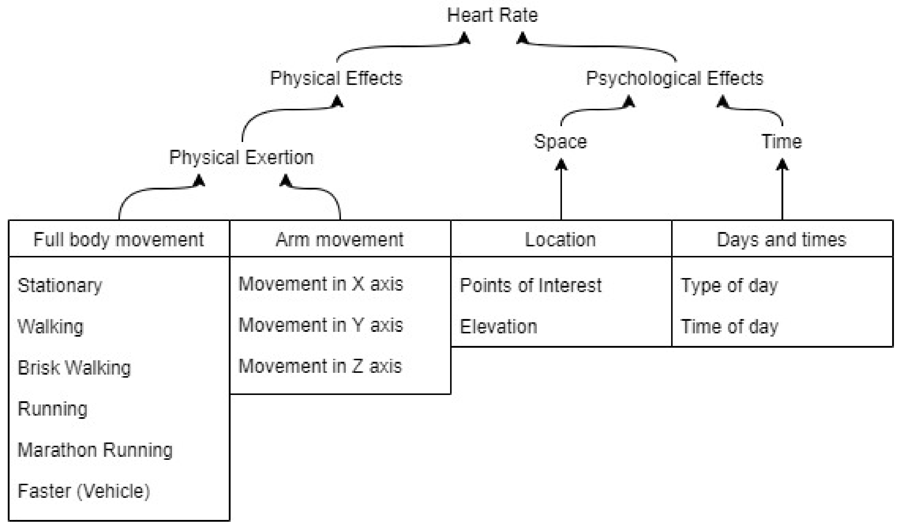
The reason why these factors were utilised was mainly due to their capacity to help deduce physical and psychological effects from one another, as can be seen in Figure 7.

Speed

To obtain the speed, the distance between the current and the last collected data point had to be found and divided by the time between them. To calculate the distance between two positional points that are collected with decimal degree coordinates, one must account for the radius of the earth to find a distance that resembles the ground truth as closely as possible. However, the radius of the earth is not consistent and fluctuates between 6353 km and 6384 km depending on where on the surface of earth the data have been collected, because of the geoidal bulge. This does not account for the above mean sea level (AMSL), and for the sake of this trial, the mean of 6371 km was determined as the mean radius of the earth. To determine the speed by each position, the speed was measured from the last point to the current point, as to reflect the speed that had affected the heart rate that was collected at the current point. The linear data of speed was divided to have six different coefficients to better understand the activity of the person. The person was deemed to be stationary between 0–1 km/h, the coefficient for this would be 0, therefore this coefficient would not be part of the model. The person was deemed to be walking (SV₁) if the recorded speed was 1–5 km/h, brisk walking (SV₂) if the speed was 5–10 km/h, running (SV₃) if the speed was 10–15 km/h, running fast (athletic) (SV₄) if the speed was 15–20 km/h, and anything faster than 20 km/h was deemed to be caused by the use of a vehicle (SV₅).

To calculate the distance between two positioning points in the data set, the haversine formula was used. The haversine formula calculates the distance between two decimal degree coordinates and accounts for the radius of the earth. The calculation can be seen in Equations (2)–(4) below. Assuming that φ₁ = Latitude point 1, φ₂ = Latitude point 2, λ₁ = Longitude point 1, λ₂ = Longitude point 2, R = the radius of Tellus; 6371 km, a = the square of half the chord length between the points, c = angular distance in radians, and d = the real distance between the points:

$$a=si{n}^2\left(\frac{\Delta \phi }{2}\right)+cos{\phi }_1\ast cos{\phi }_2\ast si{n}^2\left(\frac{\Delta \mathsf{\lambda }}{2}\right)$$

(2)

$$c=2\ast atan2\left(\sqrt{a},\sqrt{\left(1-a\right)}\right)$$

(3)

$$d=R\ast c$$

(4)

Points of Interest

For the sake of this trial, three types of point of interest were determined. Those were “office” (POI₁), “home” (POI₂), and “other,” based on geographical boundaries around the visit locations. The boundaries for each location were decided by creating a rectangle around the office and the home, which can be seen in

Table 3. The boundaries for the POIs.

Boundaries	POI1 Office	POI2 Home
Upper Latitude Limit	59.344838	59.259986
Lower Latitude Limit	59.353255	59.263847
Upper Longitude Limit	18.076021	18.079773
Lower Longitude Limit	18.054048	18.087132

.

Elevation

To obtain the elevation, each position had to be compared to a dataset containing elevation information [64]. However, the resolution of the datasets varies, meaning that the resolution of the data in the elevation dataset might not overlap perfectly with the data from the trial dataset. To account for this, an algorithm was written to find the closest location which had elevation data and utilise those data for the trial data point. This is a form of interpolation, which just copied the elevation value of the closest data point. The resolution of the elevation dataset was 30 m.

Time Categories

The type of day was categorised into weekdays (D) and not weekdays. For the time of day, three categories were chosen: “morning” (T₁) which was from 6:00 to 11:59, “afternoon” (T₂) which was 12:00–17:59, and “evening/night” which was 18:00–05:59. These categories were selected based on different time–space constraints, and, subsequently, level of stress that an individual may have on a given typical day [65,66].

Personal Biometric Model

The variables from the derived data were put together to create the Personal Biometric Model (PB-model) for effects of sensor readings on collected heart rate. The model was based on the variables described above. Time of day (T), type of day (D), and Elevation and location (POI) were used to control temporal and spatial factors. The rest of the data relating to the movement were also put in the model and a constant (C) was added, as everyone should have a base heart rate.

Thus, based on the variables listed above, the Personal Biometric Model (PB-model) employed is as shown below (the abbreviations used are described in

Table 4. Abbreviation table for the PB-model.

Abbreviation	Explanation
SVn	Dummy variables defining category of speed
Speed	Linear variable containing the actual speed of the device
AX, AY, AZ	Linear variables for the device’s movement in space
Elevation	Linear variable containing the elevation of the device
POIn	Categorical variable for predefined locations
D	Categorical variable defining type of day
Tn	Categorical variable defining time period within a day

):

$$NormHR=C+\left({\alpha }_{1}S{V}_1+{\alpha }_{2}S{V}_2+{\alpha }_{3}S{V}_3+{\alpha }_{4}S{V}_4+{\alpha }_{5}S{V}_5\right)Speed+{\beta }_{1}AX+{\beta }_{2}AY+{\beta }_{3}AZ+\gamma Elevation+{\zeta }_{1}PO{I}_1+{\zeta }_{2}PO{I}_2+\eta D+{\theta }_1{T}_1+{\theta }_2{T}_2$$

(5)

Based on the format of the model, it was possible to run it using multivariate linear regression to find the coefficients for each variable in the model, which will be presented in the results.

4. Results

This section aims to visualise and present the results from the data collection and analysis described in the previous section. The results will be described in three sections depicting each step of the analysis and the results from each.

4.1. Data Collected

Data were collected from five participants over the course of approximately three months. However, the consistency of the data varied between the participants, as some of the participants forgot about the collection and others did modifications to the hardware which interrupted the collection of data. In the end, one participant’s dataset which was most consistent and contained the most data points was chosen to be the dataset for the analysis part of this trial. In similar studies where one has tried to determine stress or cognitive load, the number of participants is usually somewhere between 15 and 35 [19,20,21,22,23,25]. However, this dataset from a single participant was deemed suitable for this study as it will give an indication of how the individual data could be used when performing the analysis. In future studies, a larger group of participants is needed, as it would give a better view of the impacts of an area.

Over the course of approximately one month, 12,495 data points were collected from said participant, a 43-year-old male. During this month, the participant travelled both domestically and abroad, which gave many data points to analyse. The participant’s heart rate fluctuation in a regular day can be seen in Figure 8.

As we can see in Figure 8, the heart rate is fluctuating throughout the day. However, the patterns during evening/night seem to differ a lot from the rest of the day. There can be many reasons as to why; however, one reason could be that the participant is not wearing the device correctly (or has even taken it off) and static noise from the environment has been collected instead. The software was supposed to control for when the device was not worn correctly and would then not collect any data, however, the possibility of the device collecting noise instead of data can still not be ruled out without further testing. However, in the time spans defined as morning and afternoon, the data seem to follow a more regular pattern, with the occasional peak. Hopefully this is an indication that correct data have been collected during that time, and for the sake of this experimental work, the assumption will be that the amount of data will be large enough for the analysis methods to disregard any errors.

Data Refinement

The data that had been collected were saved to several CSV-files and had to be compiled into one. The software that collected the data also saved data that were not relevant for this trial, such as gyroscope data. The CSV-files were combined into one large CSV-file including all data. The redundant data were deleted, and the heart rate was normalised so as to not affect the results when comparing the findings with those of other participants in the future. The date and time stamps of the data had to be individual to work with the methods of this trial. The data were filtered to only include data points from the area around Stockholm, where most of the data points were collected, which resulted in a data set of 7650 points when the boundaries were set to those in

Table 5. Decimal Degree Coordinate Boundaries.

Boundaries
Upper Latitude Limit	60
Lower Latitude Limit	56
Upper Longitude Limit	20
Lower Longitude Limit	16

.

4.2. Data Analysis

The analysis was performed as described in the methodology and, in this section, the result from each step will be presented.

4.2.1. K-Means Clustering

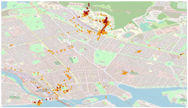
The first step of the data analysis was to find the integer to use as K for K-means clustering. This was performed with the use of the Average Silhouette Evaluation method on the whole data set, and K was determined to be 2. With K found, the dataset was clustered using the K-means clustering algorithm. The two clusters were then visualised on a map over Stockholm as can be seen in Figure 9.

4.2.2. DBSCAN

After clustering and visualising the data with K-means clustering, the two data clusters were divided into several clusters using DBSCAN, which also removed any noise and outliers from the dataset to find areas where the data collection was dense. In the cluster with regular heart rate, there were 25 spatial clusters and one layer of outliers and, in the cluster with peak heart rate, there were five spatial clusters. These spatial clusters were then compared to see where there were overlaps between the clusters and where there was not. Three of the deviation clusters overlapped with the regular pattern clusters, uncovering that, in those areas, the heart rate fluctuated. In 22 of the regular heart rate clusters, there was no overlap, and in two of the deviation clusters there was no overlap.

4.2.3. Personal Biometric Model

The data were also put through the PB-model to uncover how much each factor contributed to the heart rate readings. It showed that there had been some peaks of speed in the data which did not make sense (speeds at several thousand meters per second) and most were interpolated with the surrounding values. However, there were two points of data which had speed peaks that would not get interpolated, therefore those two points were removed from the dataset so as not to disturb the outcome of the multivariate regression using the PB-model. The results are shown in

Table 6. The results of the multivariate regression on the PB-model.

Regression Statistics
Multiple R	0.719
R Square	0.517
Adjusted R Square	0.516
Standard Error	0.149
Observations	7648

and the coefficients are shown in

Table 7. The coefficients of the multivariate regression on the PB-model.

	Coefficients	Standard Error	t Stat
Intercept	1.303	0.193	6.745
Walking	0.004	0.009	0.445
Brisk Walking	0.010	0.008	1.344
Running	0.003	0.007	0.421
Marathon	−0.001	0.004	−0.123
Faster	−0.002	0.001	−2.587
AX	−0.002	0.000	−6.012
AY	0.012	0.001	23.611
AZ	−0.008	0.000	−28.093
Elevation	−0.839	0.192	−4.379
POI1(Office)	0.076	0.005	16.127
POI2(Home)	0.295	0.010	28.943
D(Weekdays)	−0.047	0.004	−11.717
T1(Morning)	0.020	0.005	3.974
T2(Afternoon)	−0.026	0.005	−4.845

.

5. Discussion

The previous section has presented the results found using the methodology described in this paper. This section aims to explain what the results implicate, both in general and how the results matter for traffic and urban planners. This section also aims to discuss how the quality of data and the methods for data collection might have affected the results and why that matters for future trials of similar sorts, such as the one presented in this paper.

5.1. The Clustering in General

The clustering of data showed that it is possible to find locations and areas where the heart rate is consistent over time, as well as locations and areas where the heart rate deviates. The K-means clustering visualisations indicate that an increased amount of collected data points in an area give more opportunity for peak heart rates to be collected in the same area. This is further confirmed with the density-based clustering, as we can see that the areas with more significant amounts of collected data experience both deviations and regular heart rate. Further data collections should be performed in these areas with added dimensions relating to the level of stress or cognitive load the participant is experiencing. Many factors can affect how the heart rate increases and decreases in a single area, and these factors need to be found and accounted for.

However, the results of the PB-model better describe how the participant was affected and which factors played a role in it. In the following, Section 5.2, the results of the PB-model will be discussed, and in Section 5.3, there will be a discussion on the implications of these findings on urban planning.

5.2. The Results of the PB-Model

The results of the PB-model showed how the different variables affected the normalised heart rate. With an adjusted R of 0.516, one could argue that the model fits quite well, given that it is a model for human subjects with a lot of noise, however it can and should be improved in future work.

What is interesting to see is that the speed of the person is rather insignificant in the sense that its t-value is within the range for rejecting the hypothesis that it might be affecting the heart rate. For this dataset, that range would be −1.960 to 1.960 for 95% confidence. However, what must be taken into consideration is that these states are only compared to the stationary state and the data consisted of many more data points where the participant was stationary than mobile. It is also interesting to see that the higher speeds are affecting the heart rate negatively, meaning that the faster the participant has travelled, the lower the heart rate has become. By looking at the pattern of the speed coefficients, it is indicative that there seems to be a threshold where this happens. A reason for why it might be like that is, as both Gorny et al. [18] an Wang et al. [67] have concluded, that the more a participant moves their body, the less accurate a wrist-worn PPG sensor will be, meaning that if the participant is moving by themselves at high speeds, it might be difficult to read the heart rate with the device used in this study. Another reason might be that once a person has gotten into a vehicle, in theory the person should no longer be affected by the speed itself. However, a person is still susceptible to the changes in speed while in a vehicle and for future iterations of the model, both the difference in speed and acceleration should be included. However, given the control for such factors, the results of this study should show that future work might be able to obtain more accurate readings than previous studies have.

The accelerometer data indicate the gravitational pull on the participant’s device, which could be used as an indicator for the intensity of the activities being conducted. For this data collection, the sample rate was set to one sample per minute, or 0.017 Hz; however, with a higher sample rate, it would not only be possible to better understand how much a person is moving but also what type of activity is being performed if gyroscopic data were added as well. Both the software MERGEN and the PB-model should be updated to include this, as it would give a better indication of how much the activity of the person is influencing the heart rate. With the data collected, however, it is possible to see that the readings are rather significant by looking at their t-values, which might mean that there is more information to be found here.

The significance of the elevation also seems to be rather high. For this iteration of the software, no elevation data were collected with the rest of the data; it was rather gathered by comparing the spatial data to registers of elevation at specific locations. This means that only elevation changes outdoors were accounted for and no elevation changes within a building could be collected. However, the significance of this variable unsurprisingly shows that there is more information to be gathered and explored related to elevation. A variable such as elevation change since the last collected data point would give a better explanation of how the elevation is affecting the person. The absolute values being used now only show that the higher the altitudes, in general, the lower the heart rate of a person, which could be because of thinner air or other reasons.

The Points of Interest (POI) were used to show how a location can affect a person, and both POIs of the model are compared to a third category called “other,” which is neither home nor office. It is interesting to see that the persons heart rate is positively affected by both being located at home and at the office compared to other locations. Naively, this could be interpreted as if the person has an easier time being away from home and the office since the heart rate would be lower, however, that could be since the “other” category contains every other location possible within the realm of the data collection. Therefore, POIs within the “other” category could include locations which could be able to lower the heart rate, such as spas or similar POIs. This means that a broader range of POIs could be useful to find how the heart rate is affected by them. This is particularly interesting for urban planners, as they can choose their POIs as the locations where they will change or have changed the built environment to see whether the impact on the heart rate has increased, lowered, or is the same. More about this will be discussed in Section 5.3.

The weekdays and times of day are all significant variables that affect the heart rate of a person. The reason as to why the heart rate would be lower during weekdays than weekends might be because when the person is working at their office, they are less physically active than in their weekends where they might have activities which require more physical activities, such as going for walks or performing different forms of sport.

The interpretations could be further investigated by performing interviews with the participant to see whether or not they might be correct, something which could be implemented in future trials.

5.3. Implications for Urban Planning

With the results found in this trial, the framework can be found useful for traffic and urban planners. By collecting the biometric data at more locations over a longer time, it will be possible to find areas that have had participants experience both regular heart rate patterns and deviations. By analysing these areas and finding the correlation between the activities performed in the area and the heart rate, it will be possible to rule out which factors, such as walking or running, are affecting the person. When finding several areas with the same characteristics, it will then become possible to compare the features of those areas until correlations between said features and the heart rate patterns can be found. This is not unlike the works of Prelipcean et al. [4] and Allström et al. [5], to name a few; however, the difference here is that instead of just correlating activities to locations, this type of data can uncover the effects of locations. Building up a data library of such features can then help in planning future areas where the planners want no, or want to encourage, effects from the built environment on the inhabitants or travellers. With the dawn of smart cities, where every citizen can be connected to smart services, the utilisation of such frameworks as the one trialled in this paper will provide additional information on how cities can be planned to be less intrusive on the wellbeing of the inhabitants as the technology becomes available to a broader audience than before.

However, the unique selling point which needs to be addressed is the fact that these data are collected directly from the participant without any psychological interpretations handling the data before it is being collected. This is beneficial for several reasons, mainly two, which are: (1) the removal of the human factor by collecting data directly from the source leads to fewer mistakes which could have created inadequate or faulty data, and (2) the removal of the need to interpret questions from surveys also eliminates interpretation errors which could have caused data that could have been either biased or completely faulty. By measuring biometric data and referring to methods for psychophysiological extraction of mental states and conditions [19,20,21,22,23,24,25], one could reveal more reliable results given that the hardware and software used is of the best quality possible [68].

5.4. Risks

All the data analysis in this paper has been performed based on the assumption that the data have been collected correctly and that all sensors have been calibrated accordingly during the manufacturing process. That being said, there can, of course, be deviations in the data that are caused by misuse or faulty equipment, and there is no safe way to tell if this has happened. However, all deviations in the data have, for the sake of the data analysis in this trial, been treated as deviations in the sources, meaning that heart rate deviations in the collected data have been treated as ground truth deviations in the participant’s heart rate since, just as Gorny et al. [18] and Benedetto et al. [17] conclude, the aggregated data of future studies could be deemed truthful with a large enough group of participants.

The elevation data used in the data analysis had a much lower resolution than the data collected in this trial. By finding the closest value and using that, there might be many data points that share the same elevation data, when in reality the participant has walked uphill and downhill between two data points, which cannot be discovered using the current dataset. That being said, there is, of course, the possibility to redo the analysis with higher resolution data, however there will not be any possibility of collecting ground truth elevation data with the use of the chosen equipment for this trial.

By using time-dependent data collection, it has been made sure that no heart rate changes are missed in a static location; however, depending on the speed of the traveller, both increases and decreases in heart rate while travelling quickly might be missed. For future trials, a fusion of location-based and time-based collection can be used, where the software collects a sample every X meters and Y seconds, whichever comes first.

The lack of demographic data, giving information regarding health background as well as routine data such as diet and exercise programs, makes it harder to draw conclusions on the effects found when performing the analysis on a group. In this study, the data show indications on where and how the participant was affected by external factors, but that is with the assumption that no other factors play a part in affecting the participant.

6. Conclusions

The work described in this paper shows the possibility of collecting and analysing the position and biometric data collected with the software chosen for this trial:

• Machine learning methods, such as K-means clustering and DBSCAN, seem to be a viable solution for analysis of the collected data to find locations of interest;
• The PB-model can further be used to find correlations between factors in each area at specific times, to see if the physical changes are affecting the heart rate or if other types of factors related to the environment are affecting it;
• The tool is proven useful in the current state for urban planners, as they can be informed of how previous planning decisions are affecting the wellbeing of the inhabitants of an area by looking at their biometric data. By controlling for physical impact factors, as in this study, one can start to deduce psychological impact factors on travellers throughout different areas of a city.

Future directions of this work should include extensive data collection to have a more significant data set to analyse. This would include more information regarding health background, diet and other factors that might affect the heart rate which would not be psychological. However, the trial presented in this paper has given valuable information regarding the current possibilities of collecting and analysing information regarding the effects of external factors on the participant. In a study with several participants, the aggregated data could start to form a picture of how different areas are affecting travellers. By controlling for the factors mentioned in this paper, it should be possible to deduce whether the effects from surrounding environments are affecting the travellers due to physical or psychological impact. To create a more accessible, and sustainable, society, models such as the PB-model can give indications of how the urban landscape should be formed to include all possible target groups, as the dependent factor can be analysed with control for a variety of independent factors, most of which are described here.

References

1. Axhausen, K.W.; Zimmermann, A.; Schönfelder, S.; Rindsfüser, G.; Haupt, T. Observing the rhythms of daily life: A six-week travel diary. Transportation 2002, 29, 95–124. [Google Scholar] [CrossRef]
2. Chen, C.; Ma, J.; Susilo, Y.; Liu, Y.; Wang, M. The promises of big data and small data for travel behavior (aka human mobility) analysis. Transp. Res. Part C Emerg. Technol. 2016, 68, 285–299. [Google Scholar] [CrossRef] [PubMed] [Green Version]
3. Prelipcean, A.C.; Gidófalvi, G.; Susilo, Y.O. Mobility Collector. J. Locat. Based Serv. 2014, 8, 229–255. [Google Scholar] [CrossRef] [Green Version]
4. Prelipcean, A.C.; Gidófalvi, G.; Susilo, Y.O. MEILI: A travel diary collection, annotation and automation system. Comput. Environ. Urban Syst. 2018, 70, 24–34. [Google Scholar] [CrossRef] [Green Version]
5. Allström, A.; Kristoffersson, I.; Susilo, Y. Smartphone based travel diary collection: Experiences from a field trial in Stockholm. Transp. Res. Procedia 2017, 26, 32–38. [Google Scholar] [CrossRef]
6. MEILI-Travel Diary. 2017. Available online: https://appadvice.com/app/meili-travel-diary/1308940609 (accessed on 15 March 2018).
7. TRavelVU. 2016. Available online: https://www.trivector.se/it-system/programvaror/travelvu/ (accessed on 15 March 2018).
8. Ferrer, S.; Ruiz, T. Travel Behavior Characterization Using Raw Accelerometer Data Collected from Smartphones. Procedia-Soc. Behav. Sci. 2014, 160, 140–149. [Google Scholar] [CrossRef] [Green Version]
9. Empatica. Real-Time Physiological Signals E4 EDA/GSR Sensor. 2019. Available online: https://www.empatica.com/en-int/research/e4/ (accessed on 22 May 2019).
10. Fitbit, Fitbit Charge 3 Advanced Fitness Tracker. 2019. Available online: https://www.fitbit.com/charge3. (accessed on 22 May 2019).
11. Apple Inc. Apple Watch Series 3-Technical Specifications. 2019. Available online: https://support.apple.com/kb/sp766?locale=en_US (accessed on 22 May 2019).
12. Huawei Technologies Co. HUAWEI WATCH 2, NFC, Google Assistant, 4G SIM, sport watch HUAWEI Global. 2019. Available online: https://consumer.huawei.com/en/wearables/watch2/ (accessed on 22 May 2019).
13. Samsung, Gear S3 Classic. 2019. Available online: https://www.samsung.com/us/mobile/wearables/smartwatches/sm-r770nzsaxar-sm-r770nzsaxar/ (accessed on 22 May 2019).
14. Samsung, Galaxy Watch (46mm) Silver (4G LTE). 2019. Available online: https://www.samsung.com/us/mobile/wearables/smartwatches/galaxy-watch--46mm--silver--lte--sm-r805uzsaxar/ (accessed on 22 May 2019).
15. Garmin Ltd. vívoactive 3 Element Wearables Products Garmin Singapore Home. 2019. Available online: https://www.garmin.com.sg/products/wearables/vivoactive-3-element-cerise/ (accessed on 5 August 2019).
16. Wallen, M.P.; Gomersall, S.R.; Keating, S.E.; Wisløff, U.; Coombes, J.S. Accuracy of Heart Rate Watches: Implications for Weight Management. PLoS ONE 2016, 11, e0154420. [Google Scholar] [CrossRef] [PubMed] [Green Version]
17. Benedetto, S.; Caldato, C.; Bazzan, E.; Greenwood, D.C.; Pensabene, V.; Actis, P. Assessment of the Fitbit Charge 2 for monitoring heart rate. PLoS ONE 2018, 13, e0192691. [Google Scholar] [CrossRef] [Green Version]
18. Gorny, A.W.; Liew, S.J.; Tan, C.S.; Müller-Riemenschneider, F. Fitbit Charge HR Wireless Heart Rate Monitor: Validation Study Conducted Under Free-Living Conditions. JMIR Mhealth Uhealth 2017, 5, e157. [Google Scholar] [CrossRef]
19. Jerčić, P.; Sennersten, C.; Lindley, C. Modeling cognitive load and physiological arousal through pupil diameter and heart rate. Multimed. Tools Appl. 2018, 1–15. [Google Scholar] [CrossRef] [Green Version]
20. Setz, C.; Arnrich, B.; Schumm, J.; La Marca, R.; Troster, G.; Ehlert, U. Discriminating Stress From Cognitive Load Using a Wearable EDA Device. IEEE Trans. Inf. Technol. Biomed. 2010, 14, 410–417. [Google Scholar] [CrossRef]
21. Zhai, J.; Barreto, A. Stress Recognition Using Non-invasive Technology. In Proceedings of the FLAIRS Conference, Melbourne Beach, FL, USA, 11–13 May 2006; pp. 395–401. [Google Scholar]
22. Hosseini, S.A.; Khalilzadeh, M.A. Emotional Stress Recognition System Using EEG and Psychophysiological Signals: Using New Labelling Process of EEG Signals in Emotional Stress State. In Proceedings of the 2010 International Conference on Biomedical Engineering and Computer Science, Wuhan, China, 23–25 April 2010; pp. 1–6. [Google Scholar]
23. Wijsman, J.; Grundlehner, B.; Liu, H.; Penders, J.; Hermens, H. Wearable Physiological Sensors Reflect Mental Stress State in Office-Like Situations. In Proceedings of the 2013 Humaine Association Conference on Affective Computing and Intelligent Interaction, Geneva, Switzerland, 2–5 September 2013; pp. 600–605. [Google Scholar]
24. Lee, M.; Yang, G.; Lee, H.-K.; Bang, S. Development stress monitoring system based on personal digital assistant (PDA). In Proceedings of the The 26th Annual International Conference of the IEEE Engineering in Medicine and Biology Society, San Francisco, CA, USA, 1–5 September 2004; Volume 3, pp. 2364–2367. [Google Scholar]
25. Sharma, N.; Gedeon, T. Hybrid Genetic Algorithms for Stress Recognition in Reading. In Evolutionary Computation, Machine Learning and Data Mining in Bioinformatics. EvoBIO 2013. Lecture Notes in Computer Science; Springer: Berlin, Germany, 2013; Volume 7833, pp. 117–128. [Google Scholar]
26. Palmberg, R.C.O.; Susilo, Y.; Gidofalvi, G. Uncovering Effects of Spatial and Transportation Elements on Travellers Using Biometric Data. In Towards Human Scale Cities-Open and Happy; Toivonen, T., Karst, G., Willberg, E., Eds.; Department of Geosciences and Geography, University of Helsinki: Helsinki, Finland, 2019; p. 125. [Google Scholar]
27. Palmberg, R.C.O.; Susilo, Y.; Gidofalvi, G. Developing and trialling an implicit interaction platform to monitor and aiding dementia travellers. In Proceedings of the Mobile Apps and Sensors in Surveys (MASS) Workshop, Mannheim, Germany, 4–5 March 2019. [Google Scholar]
28. Li, S.; Dragicevic, S.; Castro, F.A.; Sester, M.; Winter, S.; Coltekin, A.; Pettit, C.; Jiang, B.; Haworth, J.; Stein, A.; et al. Geospatial big data handling theory and methods: A review and research challenges. ISPRS J. Photogramm. Remote Sens. 2016, 115, 119–133. [Google Scholar] [CrossRef] [Green Version]
29. Rashidi, T.H.; Abbasi, A.; Maghrebi, M.; Hasan, S.; Waller, T.S. Exploring the capacity of social media data for modelling travel behaviour: Opportunities and challenges. Transp. Res. Part C Emerg. Technol. 2017, 75, 197–211. [Google Scholar] [CrossRef]
30. Google LLC. Wear OS Overview Android Developers. 2019. Available online: https://developer.android.com/training/wearables/ (accessed on 22 May 2019).
31. Apple Inc. Watchos 5-Apple. 2019. Available online: https://www.apple.com//watchos/watchos-5/ (accessed on 5 August 2019).
32. Apple Inc. App Store-Apple. 2019. Available online: https://www.apple.com/ios/app-store/ (accessed on 5 August 2019).
33. Google LLC. Google Play. 2019. Available online: https://play.google.com/store (accessed on 5 August 2019).
34. Fitbit, Technology. 2019. Available online: https://www.fitbit.com/technology (accessed on 5 August 2019).
35. Silbert, S.; All the Things You Can Track With Wearables. Lifewire 2019. Available online: https://www.lifewire.com/what-wearables-can-track-4121040 (accessed on 5 August 2019).
36. American Heart Association. Electrocardiogram (ECG or EKG) American Heart Association. 2015. Available online: https://www.heart.org/en/health-topics/heart-attack/diagnosing-a-heart-attack/electrocardiogram-ecg-or-ekg (accessed on 20 May 2019).
37. Simjanoska, M.; Gjoreski, M.; Gams, M.; Madevska Bogdanova, A. Non-Invasive Blood Pressure Estimation from ECG Using Machine Learning Techniques. Sensors 2018, 18, 1160. [Google Scholar] [CrossRef] [Green Version]
38. Jovanov, E.; Raskovic, D.; Price, J.; Chapman, J.; Moore, A.; Krishnamurthy, A. Patient Monitoring Using Personal Area Networks of Wireless Intelligent Sensors. Biomed. Sci. Instrum. 2001, 37, 373–378. [Google Scholar] [PubMed]
39. Healthy Doc. How Does PPG Technology Works?—SoulFitBlog. 2018. Available online: https://soulfit.io/blog/how-does-ppg-technology-works/ (accessed on 20 May 2019).
40. Numenta Geospatial Tracking Learning the Patterns in Movement and Detecting Anomalies Geospatial Tracking Executive Summary Advances in Anomaly Detection. 2014. Available online: https://numenta.com/assets/pdf/whitepapers/Geospatial%20Tracking%20White%20Paper.pdf (accessed on 6 June 2018).
41. Murakami, E.; Wagner, D.P. Can using global positioning system (GPS) improve trip reporting? Transp. Res. Part C Emerg. Technol. 1999, 7, 149–165. [Google Scholar] [CrossRef]
42. Li, X.; Ge, M.; Dai, X.; Ren, X.; Fritsche, M.; Wickert, J.; Schuh, H. Accuracy and reliability of multi-GNSS real-time precise positioning: GPS, GLONASS, BeiDou, and Galileo. J. Geod. 2015, 89, 607–635. [Google Scholar] [CrossRef]
43. ASICS Digital Inc. Runkeeper—Track Your Runs, Walks and More with your iPhone or Android Phone. 2019. Available online: https://runkeeper.com/ (accessed on 6 August 2019).
44. Gonzalez, P.A.; Weinstein, J.S.; Barbeau, S.J.; Labrador, M.A.; Winters, P.L.; Georggi, N.L.; Perez, R. Automating mode detection for travel behaviour analysis by using global positioning systems-enabled mobile phones and neural networks. IET Intell. Transp. Syst. 2010, 4, 37. [Google Scholar] [CrossRef] [Green Version]
45. Reddy, S.; Burke, J.; Estrin, D.; Hansen, M.; Srivastava, M. Determining transportation mode on mobile phones. In Proceedings of the 2008 12th IEEE International Symposium on Wearable Computers, Pittsburgh, PA, USA, 28 September–1 October 2008; pp. 25–28. [Google Scholar]
46. Bohte, W.; Maat, K. Deriving and validating trip purposes and travel modes for multi-day GPS-based travel surveys: A large-scale application in the Netherlands. Transp. Res. Part C Emerg. Technol. 2009, 17, 285–297. [Google Scholar] [CrossRef]
47. Reddy, S.; Mun, M.; Burke, J.; Estrin, D.; Hansen, M.; Srivastava, M. Using mobile phones to determine transportation modes. ACM Trans. Sens. Netw. 2010, 6, 1–27. [Google Scholar] [CrossRef]
48. Prelipcean, A.C.; Susilo, Y.O.; Gidofalvi, G. A series of three case studies on the semi-automation of activity travel diary generation using smarpthones. In TRB 96th Annual Meeting Compendium of Papers, Proceedings of TRB 2017 Annual Meeting; Washington, DC, USA, 8–12 January 2017, The National Academies Press: Washington, DC, USA, 2017; p. 16. [Google Scholar]
49. Prelipcean, A.C.; Susilo, Y.O.; Gidófalvi, G. Collecting travel diaries: Current state of the art, best practices, and future research directions. Transp. Res. Procedia 2018, 32, 155–166. [Google Scholar] [CrossRef]
50. Prelipcean, A.C.; Gidófalvi, G.; Susilo, Y.O. Transportation mode detection—An in-depth review of applicability and reliability. Transp. Rev. 2017, 37, 442–464. [Google Scholar] [CrossRef] [Green Version]
51. Wang, Z.; He, S.Y.; Leung, Y. Applying mobile phone data to travel behaviour research: A literature review. Travel Behav. Soc. 2018, 11, 141–155. [Google Scholar] [CrossRef]
52. Prelipcean, A.C.; Yamamoto, T. Workshop Synthesis: New developments in travel diary collection systems based on smartphones and GPS receivers. Transp. Res. Procedia 2018, 32, 119–125. [Google Scholar] [CrossRef]
53. Gadziński, J. Perspectives of the use of smartphones in travel behaviour studies: Findings from a literature review and a pilot study. Transp. Res. Part C Emerg. Technol. 2018, 88, 74–86. [Google Scholar] [CrossRef]
54. Stopher, P.R.; Daigler, V.; Griffith, S. Smartphone app versus GPS Logger: A comparative study. Transp. Res. Procedia 2018, 32, 135–145. [Google Scholar] [CrossRef]
55. Ho Yu, C. Exploratory Data Analysis. Methods 1977, 2, 131–160. [Google Scholar] [CrossRef]
56. MacQueen, J. Some methods for classification and analysis of multivariate observations. In Proceedings of the fifth Berkeley symposium on mathematical statistics and probability, Berkeley, CA, USA 21 June 1967; Lecam, L., Neyman, J., Eds.; University of California Press: Berkeley, CA, USA, 1967; pp. 281–297. [Google Scholar]
57. Kassambara, A. Determining the Optimal Number of Clusters: 3 Must Know Methods—Datanovia. Datanovia. 2018. Available online: https://www.datanovia.com/en/lessons/determining-the-optimal-number-of-clusters-3-must-know-methods/ (accessed on 6 August 2019).
58. Kaufman, L.; Rousseeuw, P.J. Finding Groups in Data: An Introduction to Cluster Analysis; Wiley-Interscience: Hoboken, NJ, USA, 1990; ISBN 0470317485. [Google Scholar]
59. Ester, M.; Kriegel, H.-P.; Sander, J.; Xu, X. A Density-Based Algorithm for Discovering Clusters in Large Spatial Databases with Noise; Association for the Advancement of Artificial Intelligence: Palo Alto, CA, USA, 1996. [Google Scholar]
60. Galton, F. Regression Towards Mediocrity in Hereditary Stature. J. Anthropol. Inst. Gt. Br. Irel. 1886, 15, 246–263. [Google Scholar] [CrossRef]
61. Rencher, A.C.; Christensen, W.F. Multivariate Regression. In Methods of Multivariate Analysis; John Wiley & Sons, Ltd: Hoboken, NJ, USA, 2012; pp. 339–383. [Google Scholar]
62. Lai, T.L.; Robbins, H.; Wei, C.Z.; Hannan, E.J. Strong Consistency of Least Squares Estimates in Multiple Regression II*; Academic Press: Cambridge, MA, USA, 1979; Volume 9. [Google Scholar]
63. Zhang, T. Solving Large Scale Linear Problems Using Stochastic Gradient Descent Algorithms. In Proceedings of the Twenty-First International Conference on Machine Learning, SCM, Banff, AB, Canada, 4–8 July 2004; pp. 116–123. [Google Scholar]
64. Becker, J.J.; Sandwell, W.H.F.; Braud, J.; Binder, B.; Depner, J.; Fabre, D.; Factor, J.; Ingalls, S.; Kim, S.-H.; Ladner, R.; et al. Global Bathymetry and Elevation Data at 30 Arc Seconds Resolution: SRTM30_PLUS. Mar. Geod. 2009, 32, 355–371. [Google Scholar] [CrossRef]
65. Susilo, Y.O.; Liu, C. Exploring patterns of time-use allocation and immobility behaviours in the Bandung Metropolitan Area, Indonesia. In Urban Mobilities Glob. Sout, 1st ed.; Uteng, T.P., Lucas, K., Eds.; Routledge: London, UK, 2017; pp. 131–153. [Google Scholar]
66. Liu, C.; Susilo, Y.O.; Dharmowijoyo, D.B.E. Investigating intra-household interactions between individuals’ time and space constraints. J. Transp. Geogr. 2018, 73, 108–119. [Google Scholar] [CrossRef]
67. Wang, R.; Blackburn, G.; Desai, M.; Phelan, D.; Gillinov, L.; Houghtaling, P.; Gillinov, M. Accuracy of Wrist-Worn Heart Rate Monitors. JAMA Cardiol. 2017, 2, 104. [Google Scholar] [CrossRef] [PubMed] [Green Version]
68. von Watzdorf, S.; Michahelles, F. Accuracy of positioning data on smartphones. In Proceedings of the 3rd International Workshop on Location and the Web—LocWeb ’10, Tokyo, Japan, 29 November 2010; ACM Press: New York, NY, USA, 2010; pp. 1–4. [Google Scholar]
Figure 1. The process of K-means clustering.
Sustainability 13 09993 g001
Figure 2. A diagram depicting a typical elbow found using the elbow.
Sustainability 13 09993 g002
Figure 3. The iterative process of DBSCAN; red points represent core points; blue points represent border points; green points are outliers.
Sustainability 13 09993 g003
Figure 4. A diagram depicting a typical elbow found using the elbow method.
Sustainability 13 09993 g004
Figure 5. A diagram of a line function deducted from using linear regression.
Sustainability 13 09993 g005
Figure 6. Schematic of the framework MERGEN.
Sustainability 13 09993 g006
Figure 7. The relation between physical and psychological effects.
Sustainability 13 09993 g007
Figure 8. A diagram over the heart rate of the participant over the course of a day.
Sustainability 13 09993 g008
Figure 9. A visualisation of the clusters. Orange circles indicate regular heart rate; Red triangles indicate peak heart rate.
Sustainability 13 09993 g009