Abstract
Predicting evacuation demand, including its generation and dissipation process, for urban rail transit systems under disruptions, such as line and station closure, often requires comprehensive historical data recorded under homogeneous situations. However, data under disruptions are hard to collect due to various reasons, which makes traditional methods impractical in evacuation demand prediction. To address this problem from the modeling perspective, we develop a data-efficient approach to predict evacuation demand for urban rail transit systems under disruptions. Our model-based approach mainly uses historical data obtained from the natural state, when no shocks take place. We first formulate the mathematical representation of the evacuation demand for every type of urban rail transit station. Input variables in this step are location features related to the station under the disruption, as well as an origin–destination matrix under the natural state. Then, based on these mathematical expressions, we develop a simulation system to imitate the spatio-temporal evolution of evacuation demand within the whole network under disruptions. The transport capacity drop under disruptions is used to describe the disruption situation. Several typical scenarios from the Shanghai metro network are used as examples to implement the proposed method. The results show that our method is able to predict the generation and dissipation processes of evacuation demand, as well model how severely stations will be affected by given disruptions. One general observation we draw from the results is that the most vulnerable stations under disruption, where the locations peak evacuation demand occurs, are mainly turn-back stations, closed stations, and the transfer stations near closed stations. This paper provides new insight into evacuation demand prediction under disruptions. It could be used by transport authorities to better respond to the urban rail transit system disruption.
1. Introduction
The influence of unplanned disruptions, which could normally be caused by equipment failure [1,2], operation accidents, extreme weather, social public events, terrorist attacks, etc., on the transportation system, has attracted increasing attention. For massive rapid transport systems such as metro rail, disruptions may cause congestion or break down of the network. The station might become a confined space where high-densities of people gather, ultimately leading to varying degrees of casualties and hazards. Evacuation demand refers to the volume of stranded passengers and the distribution of these passengers around the whole metro rail network. Evacuation demand prediction under disruptions can support both proactive emergency plan design and real-time emergency response. The prediction information is crucial for better dispatches of the limited evacuation and medical resources.
The literature on traffic prediction under normal traffic conditions is comprehensive. However, existing methods are, in general, much less applicable in abnormal conditions [3]. Guo et al. [4] compared performances of several machine learning models under both normal and incidental conditions and concluded that historical normal patterns provided less predictive information during incidents.
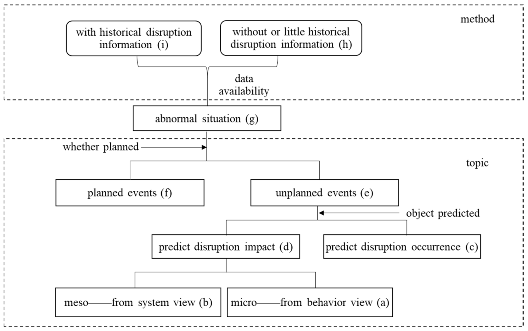
As shown in Figure 1, existing studies on traffic prediction under abnormal conditions (g) can be classified into several categories according to their topics or methods. According to the data availability, methods used in the literature could be classified into with (i) or without (h) historical disruption information. According to the event type, the literature could be classified into focusing on planned (f) and unplanned events (e). For unplanned events (e), research mainly concerns predicting the disruption occurrence (c) and its impact (d). Predicting the disruption occurrence, including its type, location, and time could help in-advance preparation [5,6]. Yap et al. [5] developed a supervised learning model to predict the expected number of disruptions per type, station, and time of day, based on the incident database of the Washington metro network. Diab et al. [6] introduced descriptive statistics and constructed statistical models using the metro system interruption data from the public transit provider in the City of Toronto, Canada. They concluded that the length of outdoor track segments in the metro system and weather conditions have a significant association with the frequency of service interruptions.

Figure 1.
Classification of the literature on traffic predictions under abnormal conditions.
When it comes to predicting disruption impact (d), the literature can usually be divided into micro-level research (a) based on passenger behavior research [7,8], and meso-level research (b), including travel demand [9,10,11,12,13], impact duration [14], and response strategies [15] of the transportation system. In this paper, we focus on predicting travel demand under disruptions at the mesoscopic level.
Guo et al. [9] investigated the impact of five meteorological features (temperature, rain, snow, wind, and fog) on transit demand including bus and rail. Silva et al. [10] used the smart-card readings covering 70 days from the London rail transit system and rich disruption records as inputs. They constructed statistical regression models to predict the exit passenger flow under disruptions. Li et al. [11] used Beijing rail transit tap-in smart-card readings to predict tap-out volume. They adopted machine learning methods and focused on improving the algorithm’s adaptability to disruption situations. Chikaraishi et al. [12] used one-month data obtained during the massive transport network disruption in Hiroshima due to heavy rain and subsequent landslides. They tested several machine learning models on traffic prediction. Hong et al. [13] established an evaluation model for the partial breakdown in rail transit networks. Taking a small-scale rail transit network as an example, they calculated impacted passenger flows under several given disruption types of the small network.
It is worth noting that previous works on metro rail evacuation demand prediction [9,10,11,12] often require a large amount of historical data under the disrupted state, however, in practice, limited by various factors, it is laborious or hardly possible to collect sufficient historical data under disruptions. For example, in many metro systems that we investigated, after the occurrence of an accident, gates must be kept open to evacuate the stranded passengers as soon as possible, leading to the missing of tap-in and tap-out records during the disruption event. Therefore, to some extent, the existing prediction methods are limited in real-world practical applications.
From the discussion above, it becomes clear that there is a need, mainly from practical perspectives, to develop a data-efficient approach which does not depend critically on historical data under disruptions. Thus, we explore the potential for evacuation demand predictions based on historical data under the normal state, which is much easier to collect. With this goal, an approach combining mathematical deduction and simulation is proposed.
The remainder of this paper is organized as follows. Section 2 describes the proposed modeling and simulation method. Stations are categorized into three types according to their location features under disruptions. Based on the origin-destination movements under normal conditions, the mathematical expression of evacuation demand for each station type is formulated. The spatial-temporal evolution of the evacuation demand is described by the simulation algorithm. Section 3 is a case study of the Shanghai metro rail network. We categorized disruption situations into eight scenarios according to the disruption features. Adopting the method in Section 2, the evacuation demand under all scenarios is calculated. The spatial-temporal evolvement of the evacuation demand around the metro rail network is also presented in the results. Finally, Section 4 summarizes the findings of the paper.
2. Materials and Methods
The disruptions we discussed refer to bidirectional closures of stations and related rail line segments. Therefore, trains are not allowed to go through the closed station and line segments in both directions.
2.1. Assumptions
Before establishing the method, we make the following assumptions.
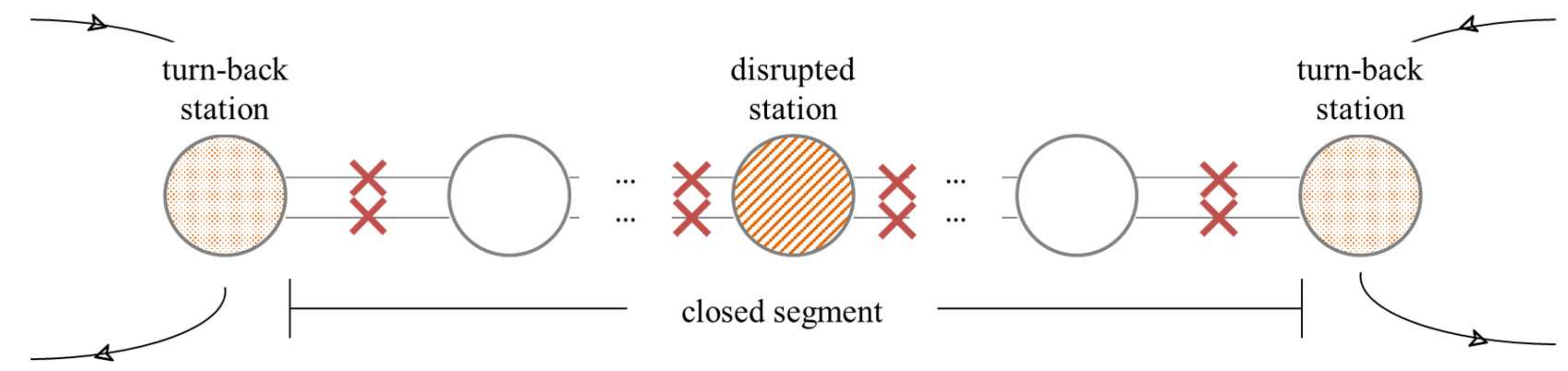
First, we assume that metro rail lines will adopt a short-turn routing operation strategy on both sides outside the closed section. After a disruption, metro rail lines usually need to reorganize their operating strategies. Here we consider a common measure, as shown in Figure 2. First, according to the location of the disrupted segment or station, two nearby stations are determined as temporary turn-back stations. The line segment between the two turn-back stations is the closed segment, which is usually wider than the directly disrupted segment. Then, trains would operate on the short-turn strategy on both ends, excluding the closure segment from its original full-length routing.
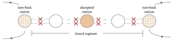
Figure 2.
Example of short-turn routing operation after disruption.
Second, we assume that passengers will not obtain information about the disruption in advance and will travel as usual. Thus, those passengers whose original travel path passing through any closed segment or station will have to get off the train when they arrive at the nearest turn-back station. This will result in an accumulation of stranded passengers at turn-back stations.
Third, we assume that passengers will always take the shortest path to their destination in the metro rail network, which is a typical behavior in routing. We do not consider the possibility of using secondary shortest routes due to the limitation of the data source.
2.2. OD Assignment in the Metro Rail Network
We modeled the metro rail network as a directed graph . The vertex set V represents the set of metro stations, and the set of directed edges E represents the set of line segments between metro stations. Specifically, an element refers to the directed line segment starting at station r and ending at station v.
The flow volume on line segment at time interval under the normal state is denoted as . For brevity, we will use an matrix to represent normal-state flow volumes on different line segments and at time intervals jointly, where is the total number of directed line segments in the network , and T is the number of time intervals in one day and its value is dependent on the time granularity. In particular, is the element at the th row and th column of .
As for the Origin–Destination matrix of the metro rail network under normal states, we will use an matrix , where is the number of OD pairs and is the number of time intervals. In particular, the element in is the demand of the i-th OD pair at time interval .
To assign the OD, demand among the metro rail network needs to determine passenger path choice. Much research has been done on passenger path choice in traffic networks. The majority of studies revolve around the UE-based traffic assignment [16]. Here, we only consider the travel time as the influence factor and assume passengers will always choose the shortest path. First, for each OD pair , we use Dijkstra’s algorithm to find the shortest travel path , which is an ordered list of tuple of directed edges and time difference . Then, the contribution of the demand at time interval to the metro rail network can be computed following the shortest path . In particular, its contribution to the network flow under normal state can be described as Equation (1).
2.3. Evacuation Demand at Different Types of Stations
2.3.1. Evacuation Demand at Closed Stations
Closed stations refer to the stations between the two turn-back stations on the same metro line (excluding turn-back stations). After the disruption event occurs, no trains are allowed to pass through the closed stations. Thus, the stranded passengers at closed stations were mainly those who originally planned to depart from the closed station. Suppose the disruption occurred at time , then the evacuation demand of the closed station at time () can be expressed as Equation (2):
where is the travel demand starting from station at time and going to station .
2.3.2. Evacuation Demand at Turn-Back Stations
Turn-back stations are stations located at both inbound and outbound ends of the closed section. Suppose the disruption occurred at time , then the evacuation demand of the turn-back station at time () can be expressed as Equation (3).
where is the set of destinations of directed edges starting from , is the set of closed stations, and is the normal-state flow volume on line segment at time .
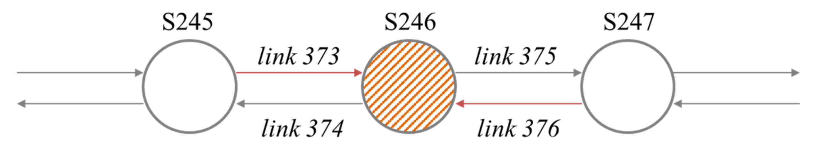
For example, consider the rail network as shown in Figure 3. Suppose that the station 246 (denoted as S246) closes at the time because of disruption, and S245 and S247 are chosen as the temporary turn-back stations. Then, passengers stranded at S245 are those who originally planned to pass through link 373 (denoted as L373) to reach S246. Similarly, passengers stranded at S247 are those who originally planned to pass through L376. According to Formula (3), evacuation demand of S245 and S247 at time () can be expressed as Equations (4) and (5).
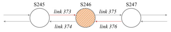
Figure 3.
Example of evacuation demand calculation for turn-back stations in the case of single station (non-transfer station) closure.
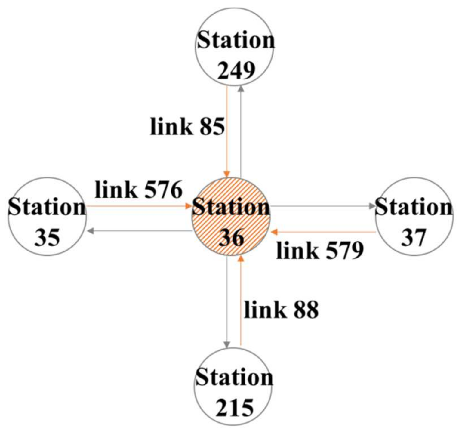
Similarly, if a transfer station is closed, then for each affected line through this station, there will be a pair of turn-back stations where stranded passengers will accumulate. For example, consider the rail network as shown in Figure 4. Suppose that the two-line transfer station S36 closes at the time because of disruption, and the stations S35, S37, S249, and S215 are chosen to be turn-back stations. Then, the evacuation demand at time () can be calculated as follows in Equations (6)–(9).
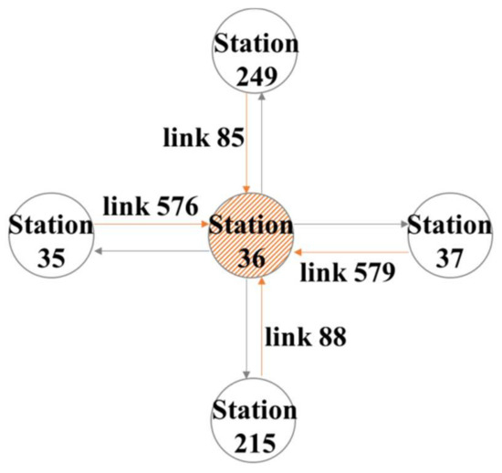
Figure 4.
Example of evacuation demand calculation for turn-back station in the case of single station (transfer station) closure.
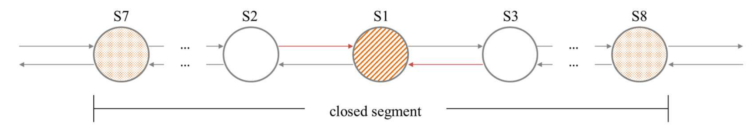
When the stations adjacent to the disrupted station are not capable of being turn-back stations, we should close these stations and reselect turn-back stations; in fact, all stations and line segments between the two chosen turn-back stations shall be treated as closed. For example, as shown in Figure 5, when S1 is closed due to disruption and its two adjacent stations S2 and S3 cannot serve as turn-back stations, we will select S7 and S8 as the turn-back stations and all segments between S7 and S8 are treated as closed.
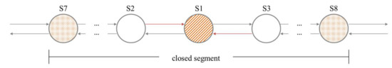
Figure 5.
Example of closed segment.
2.3.3. Evacuation Demand at OTHER Stations
Other stations refer to metro stations other than closed stations and turn-back stations. Other stations will not be directly affected by the disruption. However, after disruption occurs, passengers will redistribute in the metro rail network, and other stations may catch a sudden increase in passenger flow and be affected indirectly. In particular, if the flow volume of the metro line passing through a station reaches the maximum transport capacity, then passengers that originated from this station will not be able to get onboard and, thus, will be stranded.
Because the evacuation demand at other stations could not be expressed in closed-form equations, we use a simulation method to numerically compute them. In each time interval, the activities in the metro network can be classified into three steps: (1) passengers enter stations, (2) trains arrive at stations and passengers get off, and (3) passengers get on and trains leave stations. Our method aims at simulating these three steps. Detailed description can be found in Appendix A. As these three steps repeat themselves, the number of passengers at each station platform and on each train undergoes pulsed changes. Specifically, first, in step 1, for passengers entering stations, the number of passengers entering station at time to go to station can be directly obtained from the historical normal-state data . Second, in step 2, for trains arrivals, we check for each edge-vertex pair whether passengers on line segment arrive at their destinations or intermediate transfer locations for . Thirdly, in step 3, for trains departures, we check the remaining capacity of trains and calculate how many passengers from each OD pair can get on trains.
After 3 steps, the cycle will enter the next period and repeat itself. The detailed computation of these three steps are shown in Algorithms 1–3, respectively, with a brief introduction of the variables used in the algorithms.
3. Case Study
3.1. Input Data
The case study is conducted with the Shanghai metro rail network. We obtained smart-card data from the Automatic Fare Collection (AFC) system of Shanghai metro covering 60 days in year 2013. The dataset contains records of all trips in the rail transit system. Each tap-in or tap-out activity will leave a record, which consists of the time when the record is generated, the location code of the metro station, the transaction type (tap-in or tap-out), and the card number. The card numbers are encrypted, and are therefore anonymized but can be used to match the tap-in and tap-out activities.
We extract the normal-state OD matrix from the data by the following steps: (1) data cleaning. We discard all records that are not generated in operation time. (2) OD pairing; then, we pair the tap-in and tap-out records of the same trip. We discard records that cannot be successfully paired, such as tap-in records that cannot be matched to the corresponding tap-out records, and vice versa. (3) Aggregation; we choose 2.5 min as the time granularity and aggregate all OD pairs according to the origin station, destination station, and the 2.5 min period corresponding to the tap-in time. Then, we average the aggregated OD quantity across different weekdays to form the normal-state OD matrix . Here, we only consider weekday situations because demands during weekdays and weekends are heterogeneous, and the disruption shocks are more significant during weekdays, especially in peak hours.
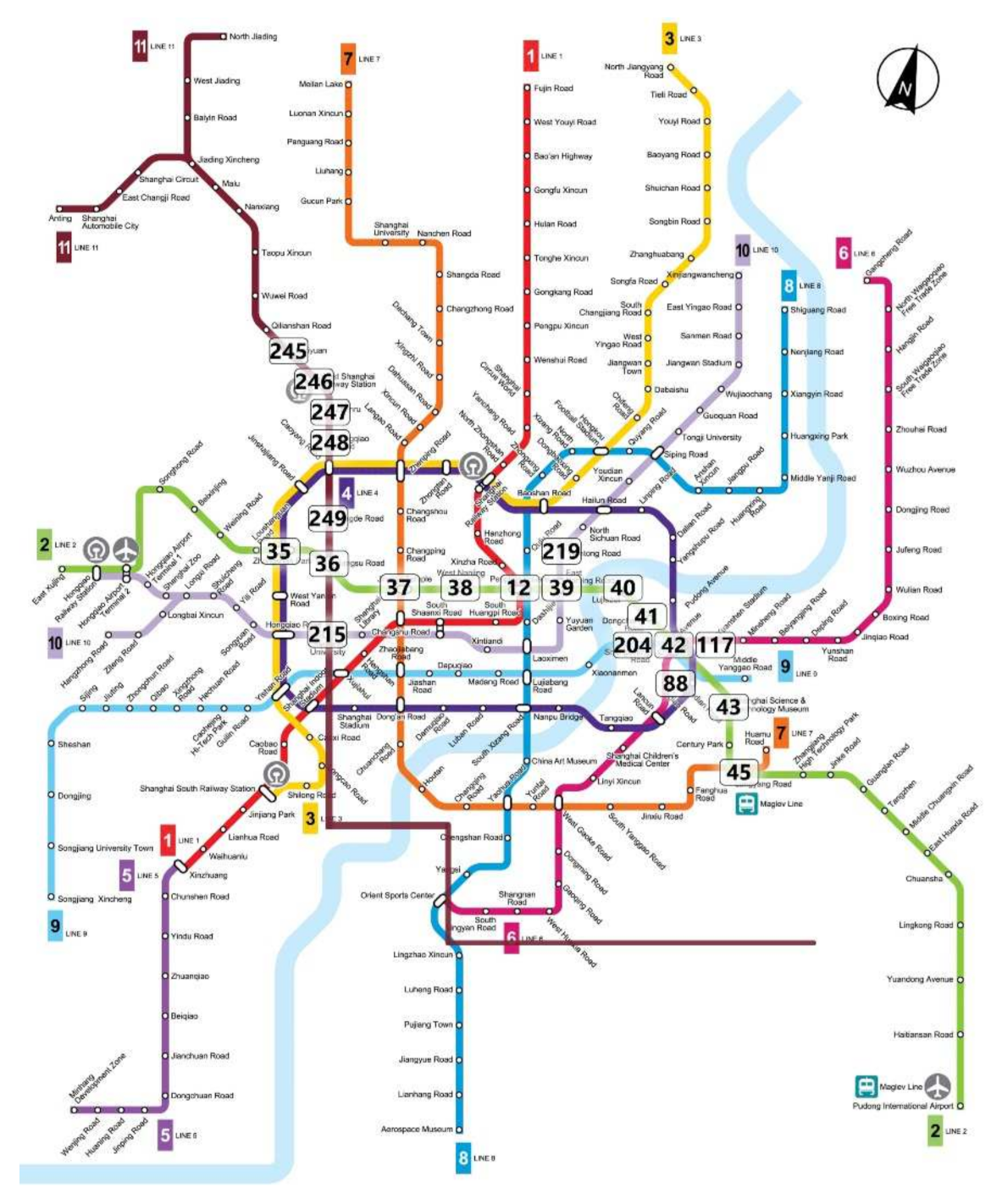
Figure 6 shows several lines, stations, and their indices of the Shanghai metro network in year 2013 that are relevant in this study.

Figure 6.
Part of Shanghai metro map in year 2013.
3.2. Prediction of Spatio-Temporal Evolution of Evacuation Demand
We apply the aforementioned simulation method to predict the spatio-temporal evolution of evacuation demand. Specifically, from the start time of the disruption event to the end of the metro operation in the day, in each 2.5-min interval, we first use equations (2) and (3) to obtain the evacuation demand at all closed stations and the turn-back stations, and then apply Algorithms 1–3 to calculate the evacuation demand at other stations.
In this study, we consider the following assumptions in the simulation:
(1) We assume that the headway between trains and the travel time between any two stations (including the train stop time at the platform) are both 2.5 min;
(2) The passenger-carrying capacity of each train in the same line is the same, which is determined according to the train’s model. Common train models adopted in the Shanghai metro system are 8A, 6A, and 6C, whose passenger-carrying capacities are 3280, 2460, and 1240 persons per train, respectively. These capacities have considered an overloaded situation;
(3) Under the normal state, the train capacity should approximately meet the travel demand. Therefore, we assume that there are no stranded passengers under normal state;
(4) In the real world, after the disruption event occurs, stranded passengers at the platform may leave the station after waiting for a long time. The maximum waiting time thresholds vary across different passengers and are affected by factors including the type and severity of the disruption event, the time when the disruption event occurs, and the personal preferences of passengers. To calculate the evacuation demand under the most unfavorable conditions, we assume that the passengers do not leave during their stranding at platforms; that is, the maximum waiting time threshold for each passenger is infinity.
3.3. Scenario Settings
We consider eight typical scenarios through orthogonal experiment design with the following binary features of disruption event: (1) whether there is more than one station closed, (2) whether the closed stations contain a transfer station, and (3) whether the disruption occurs during peak hours. The details of these scenarios are shown in Table 1. In particular, the duration of the disruption is set to 30 min, and it is from 8:00 to 8:30 when it is during the peak hour, and from 12:00 to 12:30 when it is not during peak hour.

Table 1.
Disruption Scenario Settings.
3.4. Evaluating Indicators
When modeling evacuation problems under disruptions, people usually use two types of indicators to assess the overall situation: the indicators from the perspective of passengers’ individual feelings, and the indicators from a macro system perspective.
From the perspective of individual passengers, a commonly used metric is the utility value implied by the discrete choice. For example, Saadatseresht et al. [17] pointed out that passenger perception and behavior are important factors that affect the effectiveness of evacuation measures.
Common indicators from the system perspective include per capita delay time and total evacuation time. For example, Darmanin et al. [18] and Codina et al. [19] used the above indicators as the objective in optimization problems of evacuation measures. However, Moore [15] pointed out that using the average delay time of the overall stranded population as the main indicator may overlook many other properties and, therefore, may not truly reflect the level of evacuation services.
For disruption evacuations of the metro system, the stability of the overall situation during the event is particularly important. Thus, we choose the peak demand as the main indicator. The peak demand refers to the maximum evacuation demand (number of stranded passengers) at a station within the network that may occur during the evacuation process. This indicator can reflect the severity of the overall situation and guide the evacuation response because the station at which this value appears is most likely to break down at first.
We also consider several other indicators, including the overall duration of the evacuation (possibly longer than the duration of the disruption), the number of affected passengers, total delay time, and per capita delay time, to reflect the intensity of evacuation demand and the severity of detention caused by disruption events.
3.5. Result Analysis
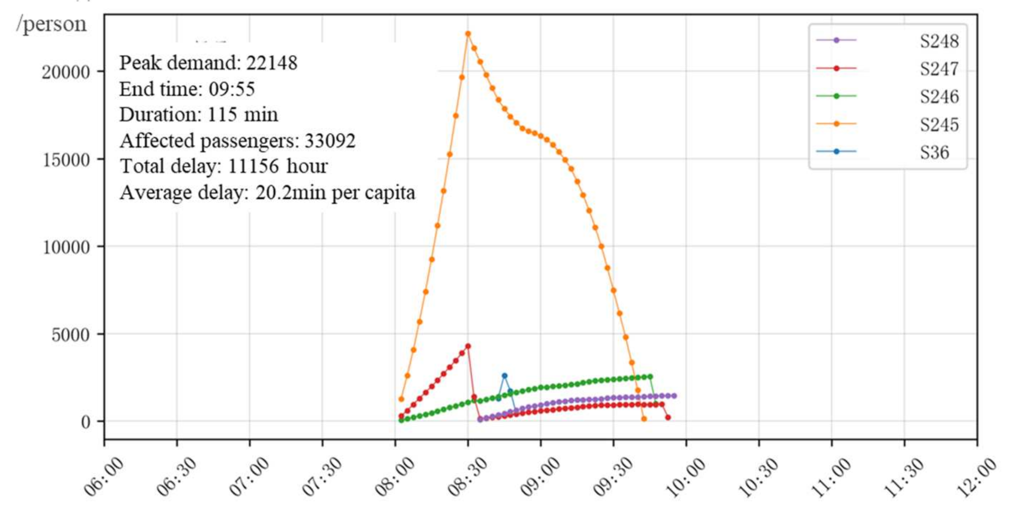
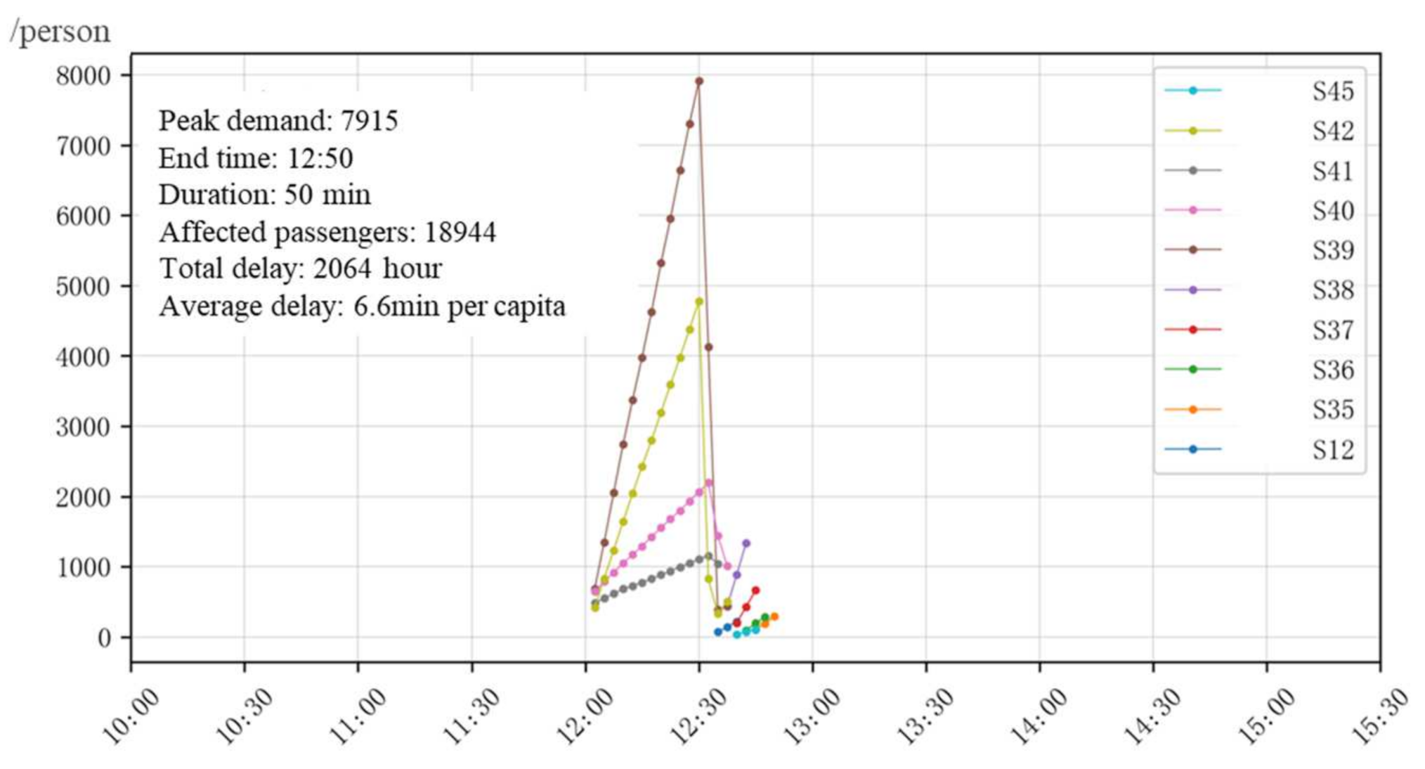
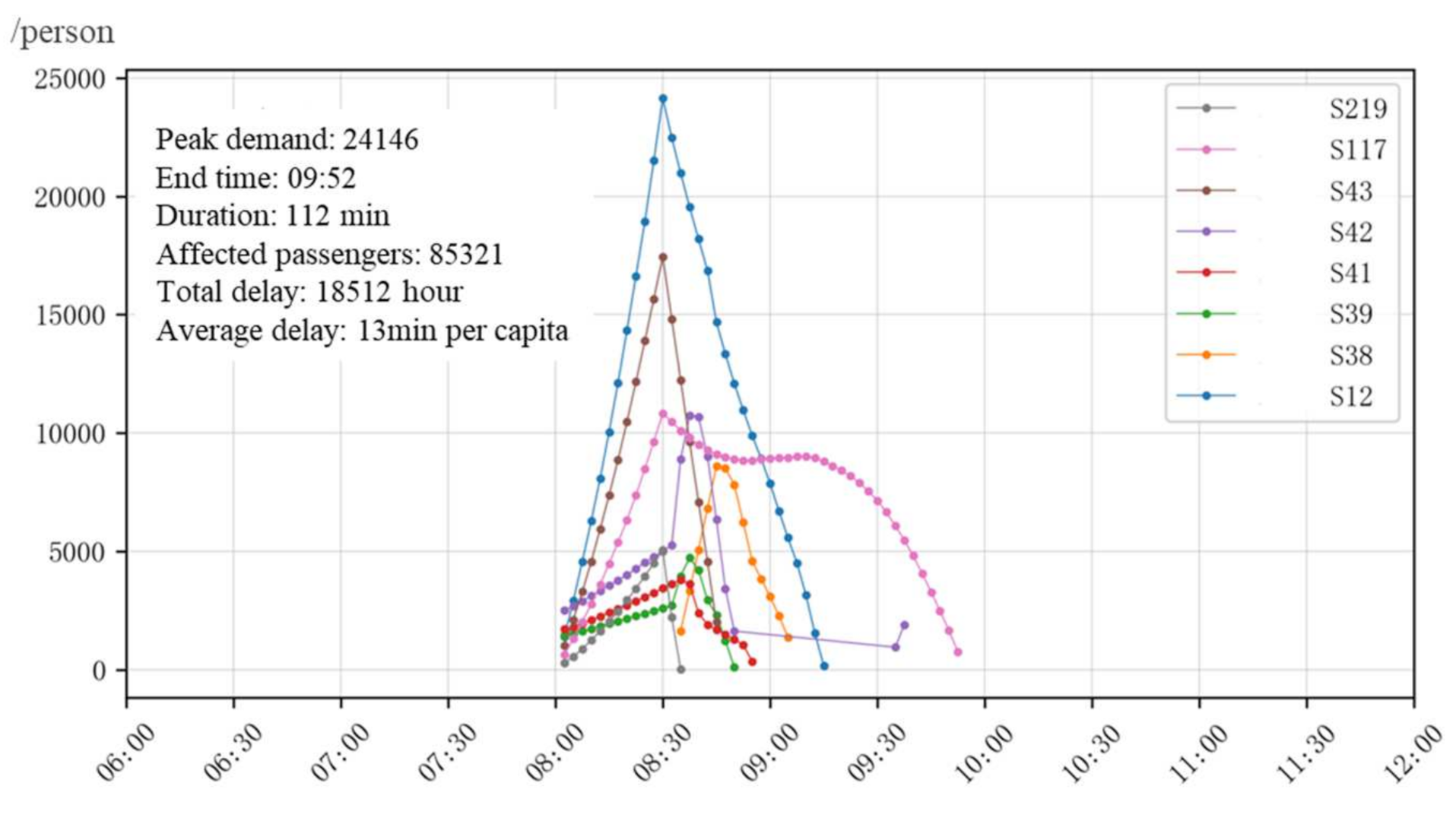
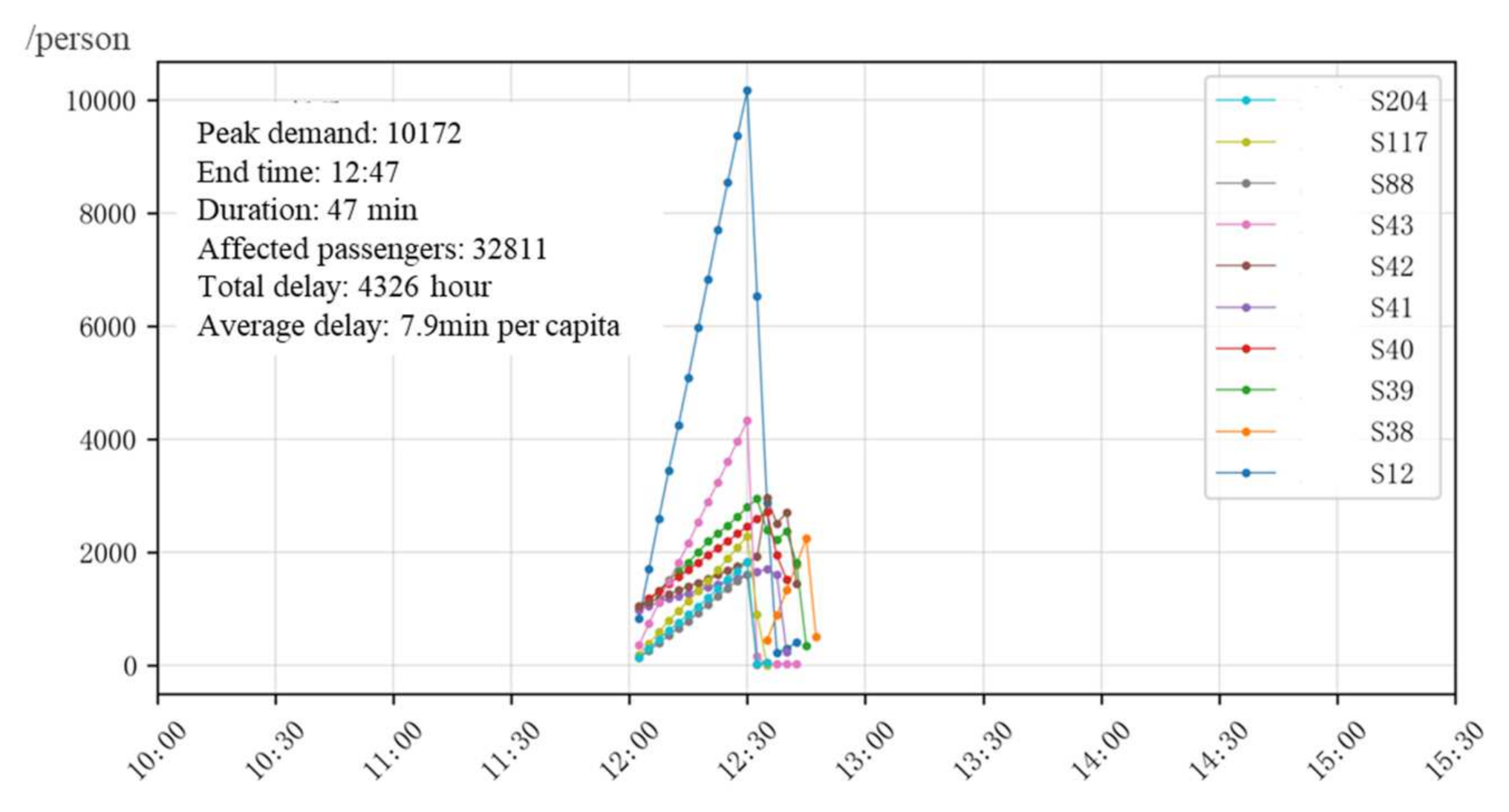
Figure 7, Figure 8, Figure 9, Figure 10, Figure 11, Figure 12, Figure 13 and Figure 14 depict the generation, accumulation, and dissipation curves of the evacuation demand under the eight experiment scenarios. For each scenario, we draw the curves of the top 10 stations with the highest evacuation demand in the entire metro network. We also calculate the peak demand and the evacuation end time, which is defined as the time when the stranded population at all stations is ignorable compared with the normal state. Table 2 summarizes those indicators in these eight scenarios.
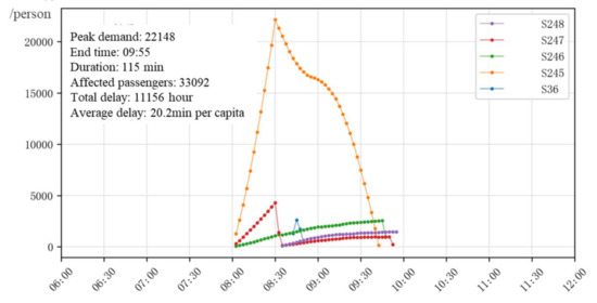
Figure 7.
Prediction result of scenario C1.
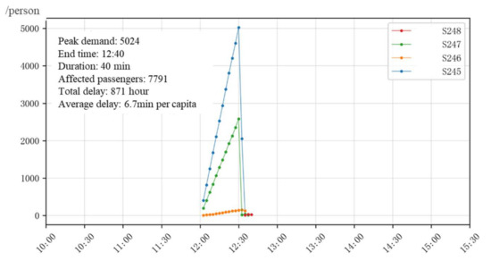
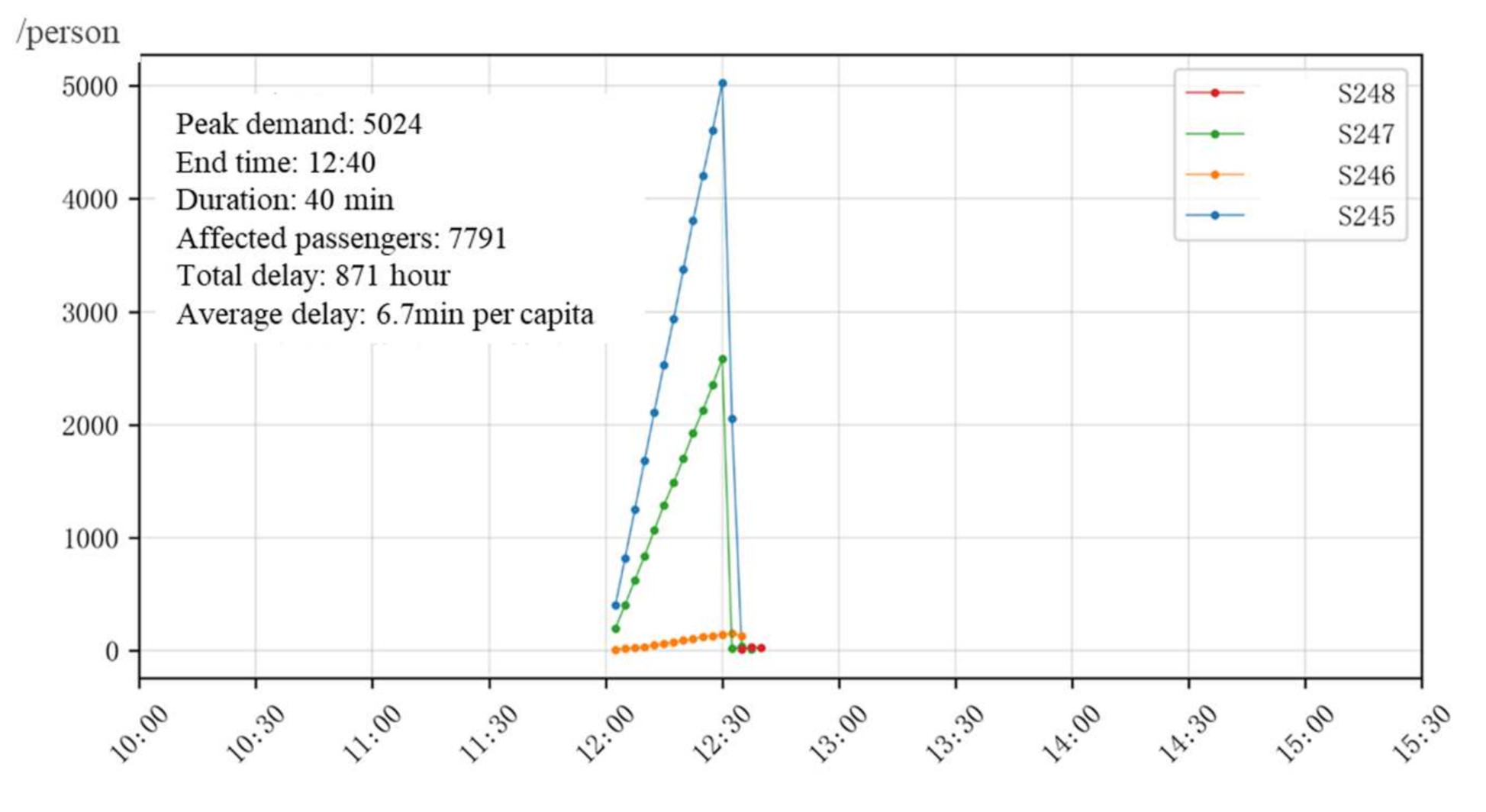
Figure 8.
Prediction result of scenario C2.
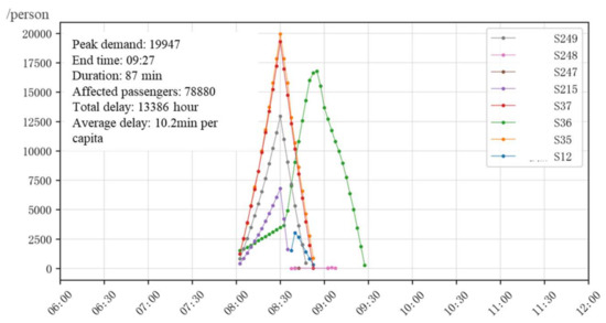
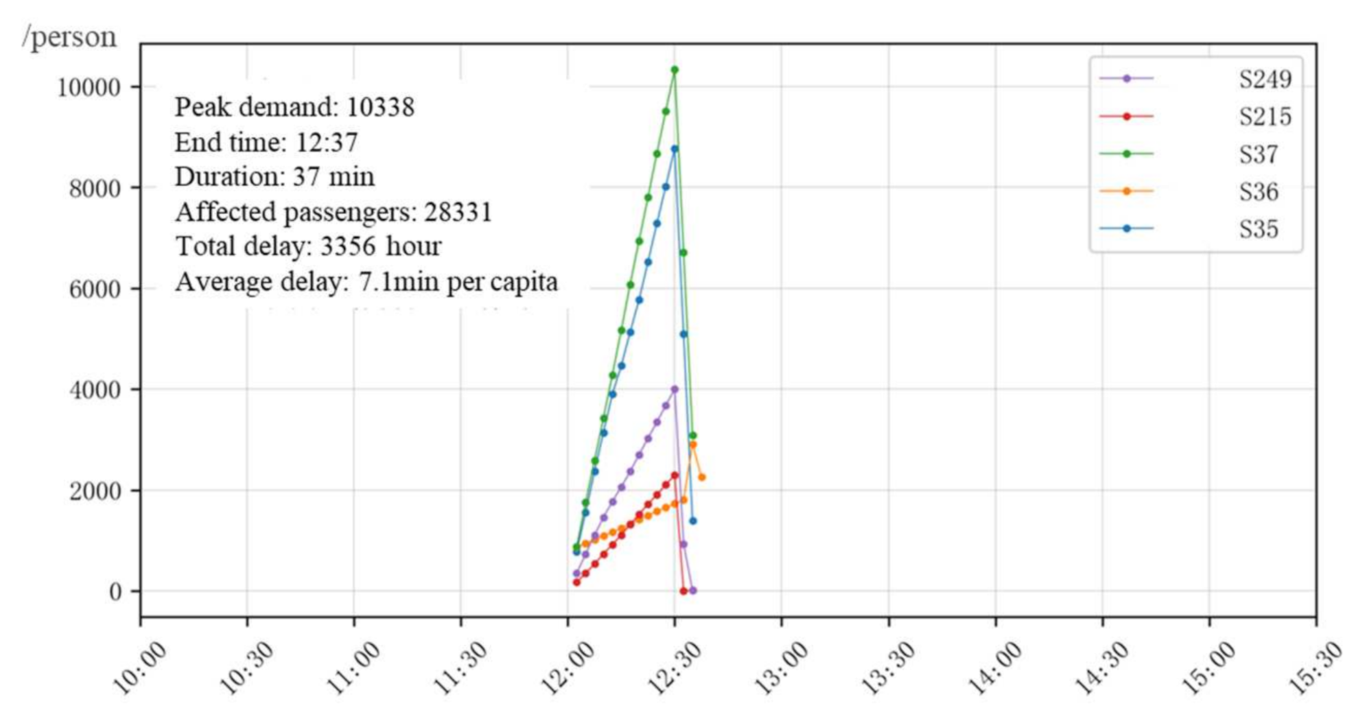
Figure 9.
Prediction result of scenario C3.
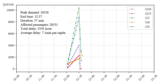
Figure 10.
Prediction result of scenario C4.
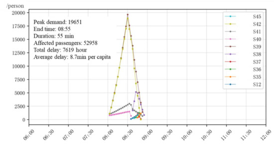
Figure 11.
Prediction result of scenario C5.

Figure 12.
Prediction result of scenario C6.
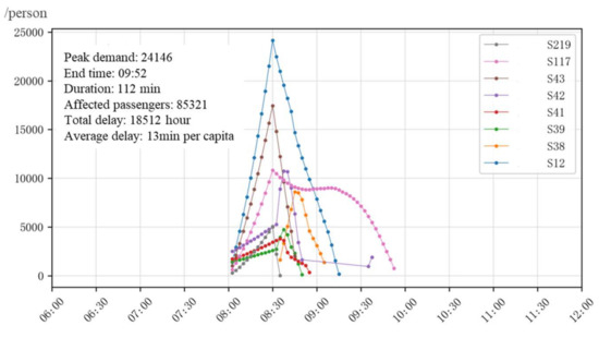
Figure 13.
Prediction result of scenario C7.
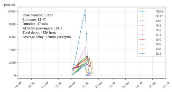
Figure 14.
Prediction result of scenario C8.
Table 2.
Evacuation demand prediction results.
Take scenario C1 and the prediction results in Figure 6 as an example. In scenario C1, the disruption event occurs during the morning peak at S246, leading to the closure of S246 at 8:00. Then, as a response to the disruption, S245 and S247 are chosen to be the temporary turn-back stations. As a result, S245 and S247 are the first stations to encounter substantial evacuation demand. Between them, the evacuation demand at station S245 is higher, because the passenger flow to the urban area during morning peak hours is higher (see Figure 4 for the direction of the line passing through station S247). The closed station S246 also generated evacuation demand, but the stranded passengers at S246 are mainly those who originally planned to depart from S246. Overall, the evacuation demand at S245, S247, and S246 continued to increase during the disruption (8:00–8:30). When the disruption event ends and S246 reopens at 8:30, the evacuation demand at S245 and S247 begins to decrease quickly. However, the evacuation demand at S246 is still increasing. Moreover, stranded passengers begin to emerge at S248. This phenomenon can be explained as follows. After the train operation is resumed, a high volume of stranded passengers at S245 get onboard, making the trains full. Then, passengers at S248 and S246 are not able to get on the train. The transfer station S36 on the disrupted line is also affected in a similar way. All stranded passengers are evacuated at approximately 9:55.
We can draw the following conclusions through the analysis of the prediction results for all scenarios:
(1) Disruption events occurring at peak hours (scenarios C1, C3, C5, C7) will induce more severe evacuation demand than disruption events occurred during off-peak hours (scenarios C2, C4, C6, C8). For the former scenarios, there are more stations being affected and higher peak evacuation demand. Moreover, the evacuation process lasts longer;
(2) Among all scenarios, those with closed transfer stations (Scenarios C3, C4, C7, C8) will have higher evacuation demand than those without closed transfer stations (Scenarios C1, C2, C5, C6). The main reason is that there are more temporary turn-back stations;
(3) The simulation results for most scenarios show that, after a disruption event occurs, the most intense evacuation demand usually appears at turn-back stations, followed by the closed station itself and the nearby transfer station. These phenomena can be explained as follows. First, turn-back stations are where the detention directly generates, so the evacuation demand intensity at the turn-back station is highest. Second, because the detention will spread along with line segments and different lines converge at transfer stations, when there are disruption events at multiple lines, the transfer stations are likely to become the main propagation point of detention; that is, the main bearer of the evacuation demand;
(4) Finally, there are some stations where the evacuation demand increases significantly after the end of the disruption event. The reason is that when the closed segment resumes operation, stranded passengers at upstream stations begin to consume the capacity of the train, so that fewer passengers at the downstream stations can get on the train.
4. Conclusions
Metro stations are relatively confined public gathering spaces. When disruption events occur, there will be high passenger density and security threats. Thus, it leads to an urgent need for the evacuation demand prediction method, to provide stranded passenger distribution and temporal-spatial evolution. The prediction information can support the evacuation decision for optimized resource allocation and dispatching.
In order to solve the above problems, we construct a data-efficient prediction method of evacuation demand for urban rail transit system under disruptions mainly based on historical data from the natural state, instead of relying on historical data under disruptions. Our method is tested by the case study using data from the Shanghai metro network. The results show that we can predict the evacuation demand and its spatial-temporal evolution among all stations in the metro network under disruptions. We also predict the peak demand value and its occurrence time and location. Our method can be applied to the decision support system of metro rail disruption management, to guide the optimization of evacuation measures.
We see our contribution compared with prior methods as follows. Previous works on metro rail evacuation demand prediction often require a large amount of historical data under the disruption stated. However, in practice, limited by various factors, it is laborious or hardly possible to collect sufficient historical data under disruptions. Therefore, to some extent, the existing prediction methods are limited in real-world practical applications. The method we propose does not require a large amount of historical data under disruptions. Instead, we use historical data under normal states, which is much easier to obtain. Thus, the applicability of our method in the real word is largely promoted.
We consider the following discussion for potential future research.
(1) With more detailed data, such as path assignment, provided by the metro authority, we can refine the OD assignment process, adding multiple path selection probabilities to consideration;
(2) In this paper, we do not take the dynamic departure process of stranded passengers into consideration. In future research, we plan to calibrate the departure curve of stranded passengers based on factors such as the station location, disruption time, and severity of disruptions, or utilize real time passenger count sensors, to further refine the evacuation demand prediction;
(3) We consider adopting this method in evaluating the effects of different evacuation measures. We can set multiple evacuation plans into scenarios and select the best plan. Thus, we can provide decision-making recommendations to optimize the response strategy and guide the stranded passengers to evacuate more quickly and effectively.
Author Contributions
X.D. and H.Q. developed the idea of the method, performed the experiment and wrote the manuscript; L.S. contributed significantly to the idea and helped perform the analysis with constructive discussions. All authors have read and agreed to the published version of the manuscript.
Funding
This research was partly funded by National Social Science Foundation of China (20ZDA086).
Data Availability Statement
Restrictions apply to the availability of these data. Data was obtained from the Shanghai metro authority and are only available with the permission of the Shanghai metro authority.
Acknowledgments
The authors would express great thanks to the Shanghai metro authority for providing the data.
Conflicts of Interest
The authors declare no conflict of interest.
Appendix A
| Algorithm A1 passengers arrive at stations |
| For #traverse all possible o For #traverse all possible d EndFor EndFor |
| Algorithm A2 trains arrive and passengers get off |
| For For #traverse all possible d If or #whether to get off the train If EndIf Else EndIf EndFor EndFor |
| Algorithm A3 passengers get on and trains leave |
| For For For If EndIf EndFor If Else EndIf EndFor EndFor |
- ——The traffic demand entering station at time to go to station
- ——The total demand entering station at time ,
- —— The total demand at station at time and planning to go to station ,
- ——The total demand at station at time ,
- ——The passenger flow to station in the train on side at time
- ——The capacity of line segment ; the total passenger onboard must not exceed this capacity
- ——the starting station of line segment
- ——the ending station of line segment
- ——the set of stations affected by the disruptions
- ——the set of time intervals when the disruptions occur
- ——the set of destinations that passengers starting from station must travel through line segment to get to
- ——total demand for boarding on the local train
- ——available capacity of the local train
- ——the previous line segment of line segment in the same metro line
- ——the next location of station in the shortest path from to
References
- Ming-yan, W.; Wang, H.; Liu, Z.G. Reach on fault tree analysis of train derailment in urban rail transit. Int. J. Bus. Soc. Sci. 2014, 5, 128–134. [Google Scholar]
- Song, Y.; Wang, Z.; Liu, Z.; Wang, R. A spatial coupling model to study dynamic performance of pantograph-catenary with vehicle-track excitation. Mech. Syst. Signal Process. 2021, 151, 107336. [Google Scholar] [CrossRef]
- Lu, Y.; Seshadri, R.; Pereira, F.C.; OSullivan, A.; Antoniou, C.; Ben-Akiva, M. Dynamit 2. 0: Architecture design and preliminary results on real-time data fusion for traffic prediction and crisis management. In Proceedings of the 2015 IEEE 18th International Conference on Intelligent Transportation Systems, Gran Canaria, Spain, 15–18 September 2015; pp. 2250–2255. [Google Scholar]
- Guo, F.; Polak, J.W.; Krishnan, R. Comparison of modelling approaches for short term traffic prediction under normal and abnormal conditions. In Proceedings of the 13th International IEEE Conference on Intelligent Transportation Systems, Funchal, Portugal, 19–22 September 2010; pp. 1209–1214. [Google Scholar]
- Yap, M.; Cats, O. Analysis and prediction of disruptions in metro networks. In Proceedings of the 2019 6th International Conference on Models and Technologies for Intelligent Transportation Systems (MT-ITS), Cracow, Poland, 5–7 June 2019; pp. 1–7. [Google Scholar]
- Diab, E.; Shalaby, A. Metro transit system resilience: Understanding the impacts of outdoor tracks and weather conditions on metro system interruptions. Int. J. Sustain. Transp. 2019, 14, 657–670. [Google Scholar] [CrossRef]
- Dai, X. Choice Behavior of Passengers in Metro Emergency Evacuation: Using Stated-Preference Data in Shanghai, China. Presented at the 94th Annual Meeting of the Transportation Research Board, Washington, DC, USA, 11–15 January 2015. [Google Scholar]
- Dell’Olio, L.; Ibeas, A.; Barreda, R.; Sañudo, R. Passenger behavior in trains during emergency situations. J. Saf. Res. 2013, 46, 157–166. [Google Scholar] [CrossRef] [PubMed]
- Guo, Z.; Wilson, N.H.; Rahbee, A. Impact of weather on transit ridership in Chicago, Illinois. Transp. Res. Rec. J. Transp. Res. Board 2007, 2034, 3–10. [Google Scholar] [CrossRef]
- Silva, R.; Kang, S.M.; Airoldi, E.M. Predicting traffic volumes and estimating the effects of shocks in massive transportation systems. Proc. Natl. Acad. Sci. USA 2015, 112, 5643–5648. [Google Scholar] [CrossRef] [PubMed] [Green Version]
- Li, Y.; Wang, X.; Sun, S.; Ma, X.; Lu, G. Forecasting short-term subway passenger flow under special events scenarios using multiscale radial basis function networks. Transp. Res. Part C Emerg. Technol. 2017, 77, 306–328. [Google Scholar] [CrossRef]
- Chikaraishi, M.; Garg, P.; Varghese, V.; Yoshizoe, K.; Urata, J.; Shiomi, Y.; Watanabe, R. On the possibility of short-term traffic prediction during disaster with machine learning approaches: An exploratory analysis. Transp. Policy 2020, 98, 91–104. [Google Scholar] [CrossRef]
- Hong, L.; Gao, J.; Xu, R. Influenced Passenger Flow Calculation under Urban Rail Emergencies. J. Tongji Univ. (Nat. Sci.) 2011, 39, 1485–1489. [Google Scholar]
- Li, R.; Pereira, F.C.; Ben-Akiva, M.E. Competing risk mixture model and text analysis for sequential incident duration prediction. Transp. Res. Part C Emerg. Technol. 2015, 54, 74–85. [Google Scholar] [CrossRef]
- Moore, A.M. A process for improving transit service management during disruptions. Ph.D. Thesis, Massachusetts Institute of Technology, Cambridge, MA, USA, 2003; pp. 177–179. [Google Scholar]
- Huang, K.; Liao, F.; Gao, Z. An integrated model of energy-efficient timetabling of the urban rail transit system with multiple interconnected lines. Transp. Res. Part C Emerg. Technol. 2021, 129, 103171. [Google Scholar] [CrossRef]
- Saadatseresht, M.; Mansourian, A.; Taleai, M. Evacuation planning using multiobjective evolutionary optimization approach. Eur. J. Oper. Res. 2009, 198, 305–314. [Google Scholar] [CrossRef]
- Darmanin, T.; Lim, C.; Gan, H. Public railway disruption recovery planning: A new recovery strategy for metro train Melbourne. In Proceedings of the 11th Asia Pacific Industrial Engineering and Management Systems Conference, Malacca, Malaysia, 7–10 December 2010; Volume 7. [Google Scholar]
- Codina, E.; Marín, A. A design model for the bus bridging problem. In Proceedings of the 12th World Conference on Transport Research, Lisbon, Portugal, 11–15 July 2010. [Google Scholar]


Publisher’s Note: MDPI stays neutral with regard to jurisdictional claims in published maps and institutional affiliations. |
© 2021 by the authors. Licensee MDPI, Basel, Switzerland. This article is an open access article distributed under the terms and conditions of the Creative Commons Attribution (CC BY) license (https://creativecommons.org/licenses/by/4.0/).