1. Introduction
Modern innovations in car-sensing devices, along with the development of deep learning techniques and recognition algorithms, has allowed engineers and researchers worldwide to implement increasingly reliable Advanced Driver Assistance (ADAS) and Automated Driving (ADS) Systems, which are expected to lead toward an improvement in road users’ safety levels (reducing the severity of injuries and/or preventing fatalities on roads), driving efficiency (e.g., vehicle fuel consumption), and, consequently, the sustainability of transportation infrastructures. The capabilities of modern cars to detect surrounding objects, represent traffic situations, and adapt their dynamic state have been enhanced to the point that some car manufacturers have first-ever presented driving automation systems capable of performing the entire dynamic driving task in a sustained manner under specific operating conditions.
Nevertheless, deaths of vulnerable road users (VRUs) continue to make for a significant percentage of all road fatalities worldwide [
1], and, consequently, more attentive actions are called for attaining the road infrastructure’s sustainability in terms of protecting VRUs. Although active safety systems are not considered driving automation as they provide momentary, not sustained, vehicle control intervention during potentially hazardous situations [
2], the European New Car Assessment Program (Euro-NCAP), the leading NCAP in the world [
3], has recently restated the key role of Automatic Emergency Braking (AEB) systems in preventing accidents that involve cars and VRUs [
4], and it has also promoted the further development of intervention-type ADAS to increase the ADS’s overall driving automation capabilities. AEB systems are vehicles’ active safety systems that assist the driver to avoid potential collisions or mitigate the severity of unavoidable impacts [
5]. These systems exploit sensors and recognition algorithms to detect vehicles, pedestrians, and other objects in the road environment that interact (or could interact) with the moving vehicle. If certain safety-critical thresholds for the interaction are exceeded and the driver does not take any evasive action, AEB systems take active control of the brakes and, in some cases, other vehicles’ subsystems (steering wheel, throttle, suspension, etc.), thereby reducing fatalities, severity of injuries, and social costs [
5,
6]. However, AEB systems generally consist of three subsystems or levels, namely “perception”, “decision making”, and “execution”, which can have quite different performance depending on the vendor/supplier that has developed it and the sensor technology used to acquire the scene data. For these reasons and to ensure adequate functioning in a wide range of traffic scenarios, AEB systems are under continuous development. In addition, some researchers have found that if vehicles were capable of understanding and anticipating the intentions (or trajectories) of drivers and nearby road users one second in advance, most traffic accidents could be prevented [
7]. In fact, such a prediction can be exploited to make appropriate driving decisions in advance, such as adjusting a vehicle’s trajectory to avoid a car-to-pedestrian accident or adapting assistance systems to the driver’s intentions (i.e., to determine, in the current situation representation, whether and when to initiate or abort an intervention, avoiding unnecessary driving interference).
Most mass-market ADAS systems do not have a medium-term predictive capability of the road users’ intentions [
8], as they are designed to act reactively in high-risk situations (particularly AEB systems). Machine learning (ML) techniques are emerging in the ADAS development field as the main approach to motion prediction [
9]. In the outlined context, ML models must learn from inputs that are time-series, e.g., the current and past positions of the traffic participants, and produce outputs that are future sequences. In recent years, Long Short-Term Memory (LSTM) [
10] and Gated Recurrent Units (GRU) [
11] architectures, variants of the more general Recurrent Neural Networks (RNNs), have shown excellent efficiency in time-series prediction tasks: these models can capture the sequences’ dynamics by extracting relevant information from an arbitrarily long context window and retaining a state of that information [
12]. Since RNNs variants are currently the preferred option for sequential data modeling, relevant LSTM- or GRU-based literature studies are presented hereafter.
Existing techniques for learning driver or other road user behavior sequences from the set of features acquired by the vehicle sensor system can be divided between two methods: classification and regression. Classification problems concern the identification of movement intention labels, which are also called “behavior primitives” [
13]: these classes segment complex driving behavior into a sequence of basic elements, such as lane keeping, left/right lane change, left/right turn, go straight, or speed maintenance, braking, and stopping. In the latter context, Khairdoost et al. [
14] implemented a deep learning system that can anticipate (by 3.6 s on average) driver maneuvers (left/right lane change, left/right turn, and go straight), exploiting the driver’s gaze and head position as well as vehicle dynamics data. Differently, regression problems are concerned with predicting the future positions of cars [
8], cyclists [
15], and pedestrians [
16] surrounding the ego-vehicle (i.e., the vehicle, also called the “subject vehicle” or “vehicle under test”, whose behavior is of primary interest in the traffic scenario), by a general understanding of their movement dynamics. Among recent RNNs applications in problems relevant to autonomous vehicle movement within urban settings, Huang et al. [
17] encoded temporal and spatial interactions between pedestrians in a crowded space by combining an LSTM and a Graph Attention Network (GAT) to obtain “socially” plausible trajectories.
Although several literature studies have attempted to evaluate the trajectories and intentions of road users, AEB systems require a Risk Assessment Model (RAM, core element of the perception level) that can objectively and quickly capture the risk level of the encounter process between the ego-vehicle and a VRU. In fact, an RAM that can fully understand the relationships between behavior and risk is essential to adequately judge the AEB system’s intervention timing and thus prevent collisions [
18]. Risk (or severity) level is intended as the potential of an elementary traffic event to become an accident [
19]. Specifically for vehicle–pedestrian (V2P) encounters in inner-city traffic (i.e., the simultaneous arrival of a driver and a pedestrian at the crosswalk or in a specific limited area), such process is a traffic event characterized by a continuous interaction over time and space between the two road users [
20] The pedestrian’s decision to enter the zebra crossing depends on the perceived speed and distance of the approaching vehicle; concurrently, the driver evaluates whether to grant or deny the priority to the pedestrian, based on the estimated arrival time at the crosswalk. Since the two traffic participants may enter a collision course during the encounter process, such a conflict has the potential to end up in a collision. For example, the latter would occur if the driver’s attention levels, his/her ability to control the vehicle, or the vehicle’s dynamic state were not adequate for a safe stopping behavior [
21].
Many researchers have addressed the issue of risk assessment for pedestrian–vehicle interactions both for current and future encounter states (for the latter, on the basis of predicted trajectories) [
7]. However, the application of traffic safety indicators, also referred to as Traffic Conflict Techniques (TCTs), has been very successful as a proactive surrogate approach (i.e., complementary to accident statistical analysis) for traffic event safety assessment, due to its efficiency and short analysis time [
22]. There are various continuous or discrete TCTs for V2P conflicts [
23]. Nevertheless, Laureshyn et al. [
19] identified and developed a set of safety indicators to continuously describe the severity level of the encounter process and, thus, to relate “individual interactions to the general safety situation” of the event. In fact, a single indicator is not sufficient to accurately classify interaction patterns into severity categories (i.e., the RAM’s purpose), as it cannot fully reflect the current safety situation [
23]. Differently, a combination of at least two indicators should be considered to properly identify pedestrian “near-accident” [
24] situations (i.e., the traffic conflicts between safe passages and collisions), which are the most relevant for pedestrian-AEB systems (PAEB), using appropriate threshold values on the selected TCTs. Among the indicators analyzed by Laureshyn et al. [
19],
Table 1 provides a detailed description of those most relevant to the discussion that follows: Time to Collision (TTC), Nearness of the Encroachment (T
2), Post-Encroachment Time (PET), and Time Advantage (TAdv).
Upon selecting safety indicators to classify near-accident events, the study by Kathuria and Vedagiri [
25] showed that TTC and PET profiles are of equal importance to effectively categorize pedestrian–vehicle interactions at unsignalized intersections into severity levels when neither pedestrian nor vehicle takes an evasive action. Moreover, Zhang et al. [
23] trained a GRU neural network to predict near-accident events at signalized intersections using PET and TTC indicators generated from videos captured by fixed cameras. The latter work is also of particular interest, as it represents the first attempt (although it was not intended for the development of PAEB systems) to implement a model capable of directly predicting the current severity level of V2P interactions, which were described by three categories: “serious conflict”, “slight conflict”, and “safe”. However, as described previously, the encounter process may have crash potential even though the two road users are not on a collision course [
19]. Conversely, the TTC calculation requires both users to be on a collision course and, thus, limits the events to be consider in safety analysis. These findings reveal that V2P encounters are extremely complicated and that, to improve the reliability of RAMs, safety indicators capable of describing the whole encounter process as a continuous interplay between vehicle and pedestrian should be considered.
The solution to this problem is offered by the supplementary indicators presented by Laureshyn et al. [
19]: namely, the Nearness of the Encroachment (T
2) and the Time Advantage (TAdv), which broaden the concepts of TTC and PET, respectively, to situations in which the two road users are not on a collision course (
Table 1). In addition, Borsos et al. [
26] recently performed a comparison of collision course indicators with indicators that include crossing course interactions at signalized intersections, demonstrating that TTC and T
2 are transferable for crash probability estimation, with stricter threshold values for T
2.
This paper presents a GRU-based system that predicts, up to 3 s ahead in time, the severity level of V2P encounters in inner-city traffic (i.e., encounters between a car and a pedestrian on a pedestrian crossing), depending on the current scene representation drawn from on-board radars’ data. A car driving simulator experiment has been designed to collect sequential mobility features on a cohort of 65 licensed university students and generate T2 and TAdv indicators for accurately classifying pedestrian safety conditions during the whole encounter process. Based on selected threshold values, the presented model could be used to label in advance pedestrians near accident events and to enhance existing PAEB systems. So, this might be a relevant contribution to improving the transportation safety.
Compared to the existing literature that has mainly focused on predicting the trajectories (or intentions) of the ego-vehicle and/or other surrounding road users [
9], the developed approach differs not only by modeling safety parameters directly related to the V2P interaction severity levels but also by the fact that the multi-step-ahead prediction depends on a low-dimensional representation of the current situation: the calibrated system depends only on six parameters related to driver mobility features and traffic scene properties. Indeed, Ortiz et al. [
13] proved that there is no need to employ the state of the actuators as features for predicting future behavior: the authors have actually predicted with simple learning algorithms (i.e., multi-layer perceptron neural networks) the braking behavior of drivers approaching a traffic light with very good accuracy at time scales up to 3 s, using as input features only the ego-vehicle speed, state, and distance to the nearby traffic light. In addition, the approach presented in this paper has some aspects in common with the research of Zhang et al. [
23], but the authors predict the instantaneous severity level (based on TTC and PET) of vehicle–pedestrian interactions whose dynamics are captured by fixed cameras placed at signalized intersections, whereas the aim of the current study is a multi-step-ahead prediction on a running vehicle.
2. Data Collection
To meet the purpose of the study, it would require the collection of mobility data on several vehicle–pedestrian encounters in real-world urban scenarios. In addition, these data must allow for the proper evaluation of interaction safety indicators (especially during an online system application) and be easily acquired by on-board sensors (i.e., cameras, pedal potentiometers, IMU, GNSS, or millimeter-wave radars). In particular, the analysis of the relevant literature [
9] allowed us to identify three main groups of features for studying the problem under analysis: the actuators and steering wheel states, the information about the car dynamics, the pedestrian speed, and the direction vector. To collect this information while keeping drivers safe, a cohort of 65 licensed university students was recruited to participate in a driving simulation experiment at the Road Laboratory of the Polytechnic Department of Engineering and Architecture (DPIA) of the University of Udine.
The use of advanced driving simulators for the analysis of driver behaviors and the development of AEB systems is an accepted and widely recognized practice [
27], since the driver’s performance observed in driving simulation shows the same patterns as real-world driving (relative validity) [
28]. Saito et al. [
29] designed and validated with a driving simulator a PAEB system that controls vehicle subsystems (brake and accelerator) in potentially dangerous or uncertain situations to decelerate the vehicle and maintain a safe driving speed. Hou et al. [
30], studying the braking behaviors of drivers in typical vehicle-to-bicycle conflicts with a driving simulator, proposed a method to improve the timing and braking phases of bicyclist-AEB systems. Bella et al. [
27] recently used a fixed-base driving simulator to evaluate the functionality and effectiveness of two types of ADAS that provide the driver with an audible alarm and a visual alarm to detect a pedestrian crossing into and outside the crosswalk.
2.1. The Car-Driving Simulator Experiment
The car-driving simulator at the Road Laboratory (product name AutoSim 1000-M) has been already validated and successfully used for studying the drivers’ braking behavior affected by cognitive distractions [
21]. The simulator cockpit is made with real car parts (e.g., dashboard, steering wheel, pedals, gear lever, handbrake, driver seat, seatbelt) of an Italian city car. These are important components of the equipment to give more realistic sensations to the driver during the simulation experiment, along with the steering force feedback, the engine sound, and the two-degree-of-freedom motion base system that reproduces the vehicle’s roll and pitch. Three 43-inch LCD screens allow the road scenario to be visually reproduced, showing a 180° view.
In the Lab’s AutoSim 1000-M driving simulator [
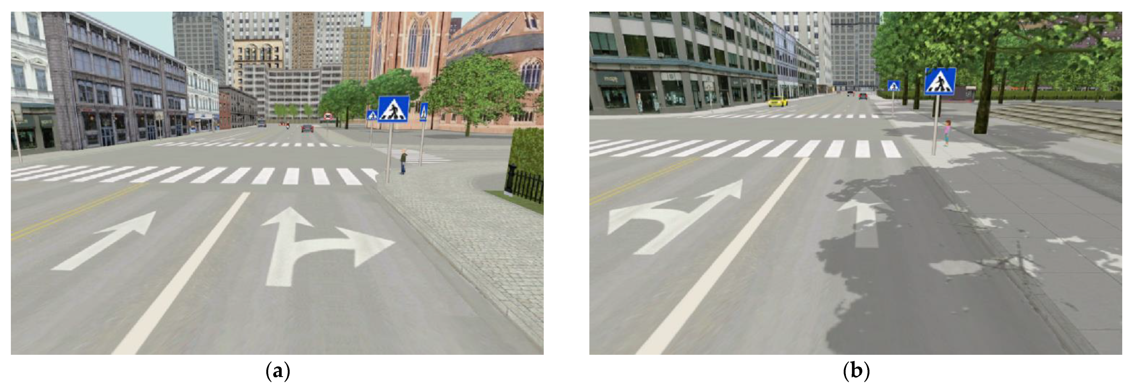
21], it was possible to record a dataset for the GRU models’ development by observing test participants’ behavior toward two planned traffic encounters: a boy/girl entering a crosswalk from the curb. The simulated scenes (
Figure 1) were set in a typical urban environment on a course that could take about 15 min to be completed, considering the 50 km/h speed limit. On the urban course, participants experienced many traffic light intersections, tight turns (90°), short straight streets, and occasional crossings of pedestrians, some of which occurred outside the crosswalks. The encounters that were used to record data (and compute surrogate safety indicators for each participant in an offline fashion, following the procedure described in Appendix A of the study by Laureshyn et al. [
19]) were set on a four-lane road (two lanes in each direction), placing traffic signs and markings that met European standards (
Figure 1).
The scenarios were designed as follows: (1) the participant arrives at a red traffic light approximately 200 m from the crosswalk, on which he/she has a clear view; (2) as the participant starts driving, the pedestrian (initially hidden) walks at a 90° angle toward the road and then stops at the edge of the curb; (3) at the moment the vehicle, based on its current speed, is about 3 s from the crosswalk, the pedestrian enters the zebra crossing and maintains a speed of 1.4 m/s. These conditions, consistent with relevant literature [
31], require the participant to stop, giving priority to the pedestrian. In this way, the data collected refer to stopping maneuvers that avoided a collision with the pedestrian.
2.2. Partecipant Statistics and Experimental Procedure
The students recruited for the experiment were between the ages of 20 and 30, had a valid driver’s license, and had driven at least 5000 km in the past year. All participants were properly trained in the use of the simulator actuators before the experimental driving and were able to test their abilities on a simulated suburban course that took approximately 5 min. Before the urban driving simulation, each participant filled in a questionnaire aimed at collecting his/her personal data (e.g., age, driving experience). Conversely, at the end of the simulation test, a second questionnaire about the discomfort perceived while driving was completed by each participant to identify and remove from the cohort those drivers who had experienced excessive annoyance. The simulation test procedure just presented has been drawn from relevant literature that provided for its validation [
21,
27,
31]. The recruited cohort includes 19 females and 41 males, with a mean age of 24.0 (SD 3.43) and 24.1 (SD 1.91) years and a mean non-verbal intelligence quotient (IQ) [
32] of 33.4 (SD 2.50) and 33.9 (SD 1.66), respectively. Therefore, the sample of males and females can be considered roughly balanced for age and IQ. However, the original cohort had an additional five participants who were excluded from the analyses, as they could not complete the experiment due to excessive discomfort.
It is worth pointing out that participation in the experiment was voluntary, there was no monetary reward, and all participants gave informed consent after being instructed on the simulated driving test procedure. Conversely, they were not informed about the objectives of the research. Finally, the study has been conducted in accordance with the Declaration of Helsinki, and the protocol was approved by the Local Ethics Committee of Udine’s University (Progetto_Guida).
2.3. Problem Formulation
Formally, the severity prediction system has to perform a mapping between the situation representation at the current driving time
, i.e., the real-time scene properties and vehicle status described by a set of sensor-observed features, and the expected severity level of the vehicle–pedestrian encounter, which is defined by T
2 and TAdv, for times
+ 1s,
+ 2s, and
+ 3s. In practice, a learning algorithm is trained to accurately predict the surrogate safety indicators at instants
2s,
1s, and
using the vehicle sensing system observations available at instant
3s. Once the expected convergence between predicted outputs and ground-truth targets is reached, the trained model represents the desired medium-term prediction system and can be used to make forward-in-time predictions based on the current scene representation. It is assumed that the input features can all be acquired simultaneously and at a regular time interval given by the lowest sampling frequency among those of the involved sensors, since the goal is to perform real-time prediction on running vehicles. However, considering that the current study is based on a driving simulator experiment, the calculation of surrogate safety indicators for each participant and the training of the learning algorithm were both performed in an offline fashion (please refer to Appendix A of the study by Laureshyn et al. [
19]) at the end of the driving experiments.
2.4. Low-Dimensional Input Representation
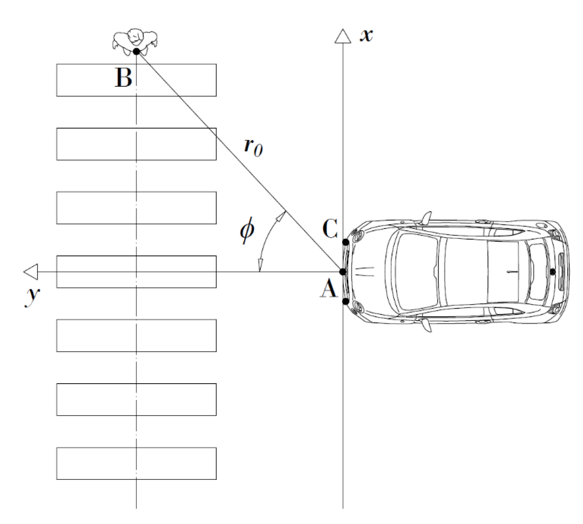
The coordinate system established for the vehicle sensing system is shown in
Figure 2. The following features form the six components of the learning model input vector and describe the V2P interaction process at the current time
for each participant in the experimental data set: driver’s behavior primitive
, current
value, ego-vehicle’s speed
, pedestrian’s speed
, and position vector (
).
Behavior primitives are the set of elementary behaviors into which the driver’s approaching maneuver (in the longitudinal dimension of the event) can be segmented based only on speed, gas pedal, and brake pedal information [
13]. These data, easily acquired on modern vehicles (e.g., by means of pedal potentiometers, IMU, GNSS), are processed to define a categorical variable whose values, in the case of V2P conflicts, are 0 for “stopped behavior”, 1 for “braking behavior”, and 2 for “maintaining speed behavior”. Based on the study by Ortiz et al. [
13], the parts of the stream wherein the vehicle speed
is less than 2 km/h (about 0.56 m/s) are labeled “stopped”. The “braking” behavior begins at the moment the driver releases the gas pedal completely, since in urban traffic, this condition represents the beginning of slowing down in response to an event. All other moments in the stream that do not belong to the two illustrated categories are labeled as “maintaining speed”. The categorical variable of behavior primitives represents important information for the GRU model, as it allows the sequence of mobility features to be segmented according to the current driver behavior. Similarly, the current value of T
2, which can be calculated directly using the other features as shown by Laureshyn et al. [
19], is of high importance, since neurosciences indicates that the human brain relies closely on judgments of TTC (and, consequently, of T
2, since the two indicators are transferable [
26]) to perform coordinated action [
33].
Position vector components are the azimuth angle
of the pedestrian with respect to the travel direction and the distance
between the ego-vehicle (point A or C) and the pedestrian (point B, please see
Figure 2). Specifically,
,
, and
are the pedestrian state data acquired by millimeter-wave radars mounted on the vehicle front end (points A and C,
Figure 2). In fact, since the detection of the pedestrian presence in the scene is usually performed using robust frame classification algorithms on vehicle camera videos [
34], the status of the detected pedestrian can be easily acquired by radars: in this study, we assumed data acquisition equipment consisting of a long-distance millimeter-wave radar installed at the center of the vehicle front end and a mid-range radar on either side of the vehicle front, with maximum detection distances of 100 m and 50 m and azimuth angles of ±10° and ±45°, respectively, to ensure the optimal scene coverage [
18]. Compared to video sensors that require object tracking and perspective transformation after object detection to generate the trajectory profiles of VRUs in time-series [
23], radars allow the direct and continuous acquisition of pedestrian mobility features [
18]. However, the use of cameras is essential for pedestrian detection in the traffic scene; in this regard, for the further online analysis of the proposed system, the use of the state-of-the-art Mask R-CNN (Region-based Convolutional Neural Network) [
35] is recommended to ensure high performance of the automated object detection process.
Therefore, time sequences of participants’ maneuvers begin with the detection of the pedestrian’s status from the long-distance radar, approximately 100 m from the crosswalk, assuming the simultaneous recognition of the pedestrian’s presence by the ego-vehicle detection model. Time sequences end when the first road user (the pedestrian) leaves the conflict zone or the second road user (the driver) comes to a complete stop, and none of the TCTs can be calculated (since the collision is no longer possible). Furthermore, although the sampling rate of radars (e.g., the current 77 GHz band millimeter-wave radar) is 20 Hz, we assumed that the encounter process is recorded at 10 Hz to account for limitations of other on-board equipment and raw data processing times.
2.5. Safety Indicators and Severity Classes Generations
Regarding the model output vector, we decided to split the severity level prediction problem into single-output learning tasks: T
2 continuous values and TAdv categories were the learning target of two distinct GRU models. Although both safety indicators can be calculated continually over time, TAdv does not provide the same smooth transfer between crossing and collision courses as T
2: conversely, it quickly goes to zero and holds that value as long as the two road users remain on a collision course (since, by definition, TAdv cannot take on negative values). After the change from collision to crossing courses due to the driver’s braking or slowing down, the TAdv value starts gradually growing. Such a behavior induces singularities in the TAdv pattern during the maneuver (i.e., if TAdv is plotted on a graph as a function of time, it will not make a continuous curve), which are difficult to capture with ML regression techniques, unless overfitting the model. To avoid running into such problems, TAdv values less than 1s have been labeled as “collision course” and those greater than 1s have been labeled as “crossing course”, since this indicator can be interpreted as the minimal delay of the driver that, if applied, will result in a collision course [
19]. Conversely, T
2 is defined by a continuous curve over time and provides information about how soon the encroachment will occur. Thus, the TAdv prediction is treated as a binary classification problem, whereas the T
2 prediction represents a regression problem.
After training these models separately, their predictions were used to classify conflict interactions ahead in time, distinguishing between “safe” and “unsafe” processes. These categories have been defined according to the static threshold values reported in the literature [
23,
26,
36,
37] and the conditions under which the simulation experiment was performed [
31]: when the TAdv class is “collision course” and the T
2 value is less than 3 s over the same time horizon, the interaction is defined as “unsafe”; in all other cases, it is considered “safe”. Additional intermediate classes have been avoided (e.g., the case wherein TAdv is reporting “collision course” but the T
2 value is greater than 3 s), since the main interest is to detect actual hazard situations or “serious conflict” iterations ahead of time (i.e., before they happen) [
23]. By comparing the models’ results with the ground-truth targets, it was possible to evaluate the effectiveness of the proposed system in classifying pedestrian’s near-accident events. However, an additional GRU neural network has been developed to directly predict the severity level of V2P encounters to verify which of the proposed models would guarantee the best classification performance.
It is worth recalling that the procedure reported in Appendix A of the study by Laureshyn et al. [
19] has been applied for the offline calculation of TCTs. In addition, the dimensions of the simulated vehicle were considered in calculations so that, among all the pedestrian–vehicle front-end contact points in a potential collision, the one leading to the lowest T
2 and TAdv values has been selected. Then, the obtained values were time-translated (by 1, 2, and 3 s backward) to compose the ground-truth target matrix.
Finally, before being inputted to the GRU, each feature (and target) was standardized; i.e., it was subtracted by its minimum value and divided by the distance between its minimum and maximum value computed on the training set, to remain in an acceptable range with respect to the activation functions.
4. Results
The aim of this study was to develop a GRU model that could predict, up to 3 s ahead in time, the level of severity of vehicle–pedestrian encounters in inner-city traffic. In this regard, two equivalent approaches have been identified [
9], i.e., (1) using multiple GRUs to separately model the supplementary safety indicators (T
2 and TAdv) that allow the interaction severity to be estimated, or (2) using a single Recurrent Neural Network as a sequence classifier to directly label near-accident events, based on relevant mobility features of V2P encounters. It is worth pointing out that although the two approaches considered are equivalent from the standpoint of the final outcome (i.e., the prediction of severity levels ahead in time), Approach (1) would allow more flexibility in labeling the pedestrian’s near-accidental events, since TCTs’ threshold values that are different from those considered in this study could be selected to classify the risk level of V2P interactions (e.g., using specific threshold values for geographic contexts of system operation, which are derived from studies of local/national driving behaviors) [
23]. In what follows, we refer by the acronyms GRU
T2 and GRU
TADV to the GRU models predicting T
2 and TAdv, respectively. Differently, to make the comparison between the two approaches presented previously, the severity classification model resulting from Approach (1) is presented as M-GRU
SL, whereas that of Approach (2) is presented as S-GRU
SL.
In this section, the generalization capabilities of the trained models are evaluated for each time horizon (i.e., 1 s, 2 s, 3 s ahead) based on commonly used evaluation metrics, which are different for classification (i.e., Accuracy, Precision, Recall, Specificity, False Alarm Rate (FAR), and Area Under the Curve (AUC)) and regression problems (i.e., Mean Absolute Error (MAE), Mean Absolute Percentage Error (MAPE), Root Mean Squared Error (RMSE)), and averaging their scores over the five test folds. These metrics are briefly presented throughout the discussion to make the models’ evaluation clearer to the reader; however, more detailed descriptions can be found in [
9,
23,
47]. Moreover, to prevent predictions from reacting with a delay especially for longer time horizons [
8], an additional metric to evaluate T
2’s time-series regression, which is usually applied in multi-step-ahead prediction problems [
47], has been considered, namely the Modified Index of Agreement (
) [
48]. In fact,
is able to concurrently consider differences in observed and predicted means and variances, providing a better evaluation of model predictions than traditional metrics.
After comparing the models’ performance under different hyperparameter combinations, the most appropriate values for each GRU model have been selected: the initial learning rate is set to 0.001 for the GRU
TADV model and 0.005 for both GRU
T2 and S-GRU
SL models, whereas the learning rate drop factor is 0.8 for all considered models. The unit number
within the GRU memory is 64 for GRU
T2, 256 for GRU
TADV, and 128 for S-GRU
SL.
Table 2 and
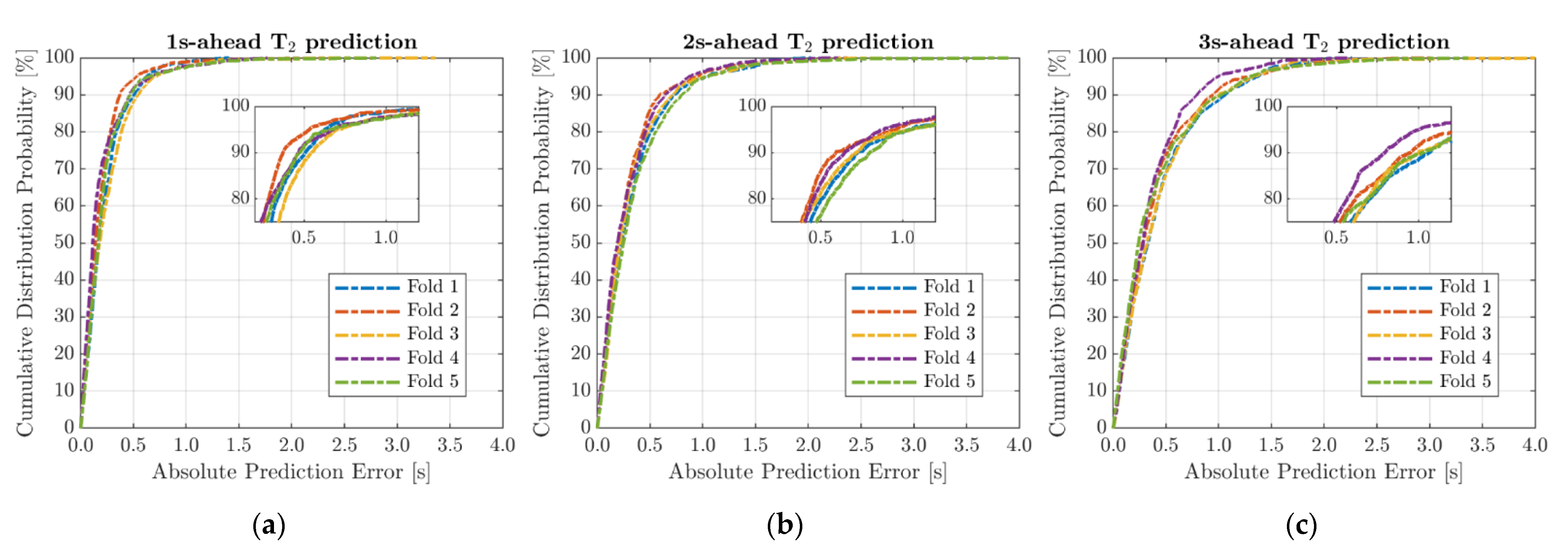
Table 3 present the evaluation metrics scores, validated on the five test folds, distinguishing by model and prediction time horizon (standard deviations on the five folds are shown in brackets). In addition,
Figure 4 presents the empirical cumulative distribution probability (ECDP) of the absolute prediction error over each fold for the GRU
T2 model. Conversely,
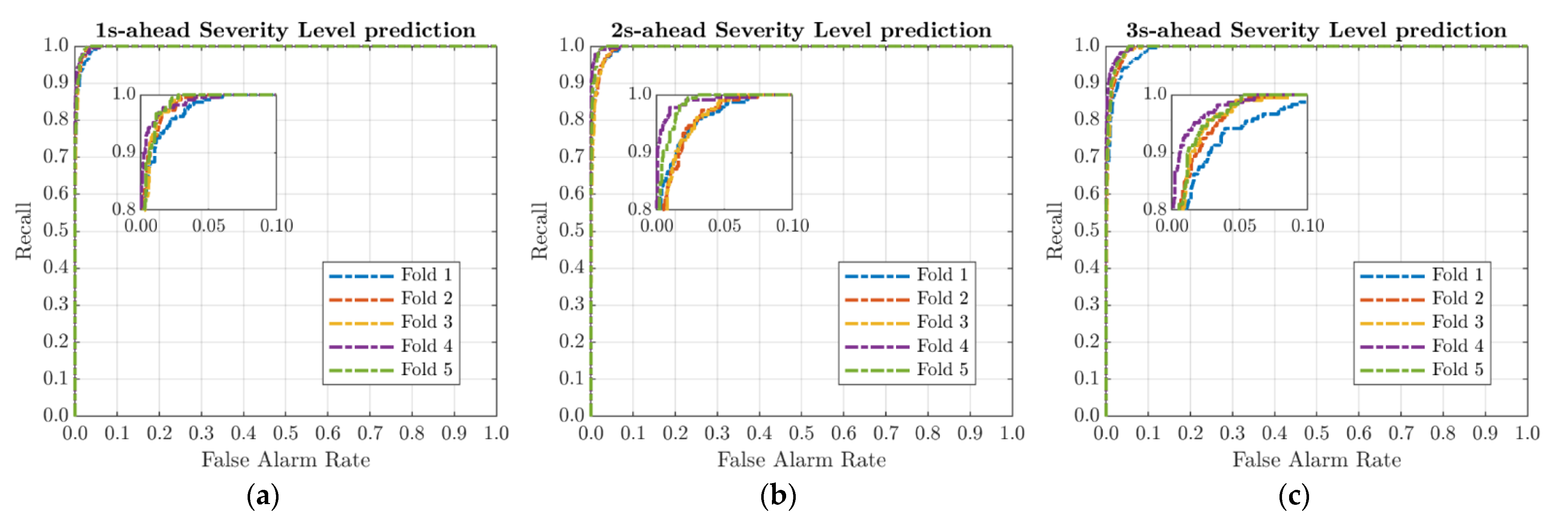
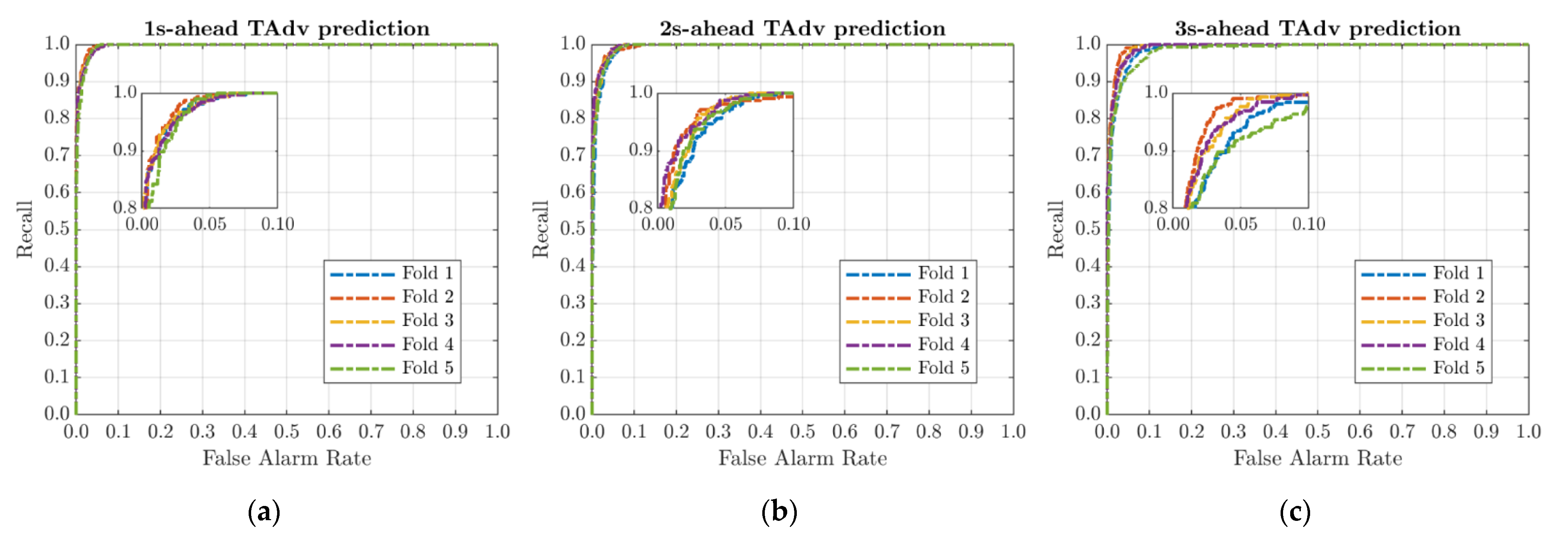
Figure 5 and
Figure 6 show the Receiver Operating Characteristic curve (ROC) for the GRU
TADV and S-GRU
SL models, respectively. This curve, which plots recall as a function of FAR, is a comprehensive metric to evaluate classification models’ performance [
23], since the closer the area under the ROC curve (AUC) is to 1, the better the prediction quality. Finally,
Table 4 summarizes the performance of the severity classification models, M-GRU
SL and S-GRU
SL, averaging the test results over folds and time horizons.
As expected, the quality of predictions increases if the time horizon decreases, no matter which model is considered. This result suggests that there is a strong correlation between the selected mobility features at time
and the desired target at time
+1. In contrast, this correlation becomes weaker for longer time horizons, and as a result, distinguishing the expected target becomes more difficult. For example, considering the GRU
T2 model (
Table 2), all evaluation metrics get slightly worse as the time-step gets longer both in training and testing stages. However, focusing on the test RMSE (column 5,
Table 2), i.e., the square root of the mean squared difference between predicted and observed values, its worsening is characterized by a deviation close to one-tenth of a second: the maximum deviation, equal to 0.138 s, is measured moving from the 1s (RMSE = 0.327 s) to the 2s (RMSE = 0.465 s) prediction time-frame, whereas the prediction quality worsens by 0.122 moving from 2 s to 3 s (RMSE = 0.587 s). Therefore, the results obtained are on the whole satisfactory, as also shown by the other parameters: the test MAE (column 3,
Table 2), i.e., the mean absolute error, was on each time scale less than half a second; the 90th percentile of the absolute error (
Figure 4), i.e., the value of the prediction error (in absolute value) which is exceeded in no more than 10% of time sequences, is equal to 0.472 s (averaged over the five folds) at the 1 s, 0.696 s at the 2 s, and 0.967 s at the 3 s prediction time-frame; the
parameter is always greater than 0.850 whatever the prediction time horizon, proving the close agreement between the observed and forecast curves.
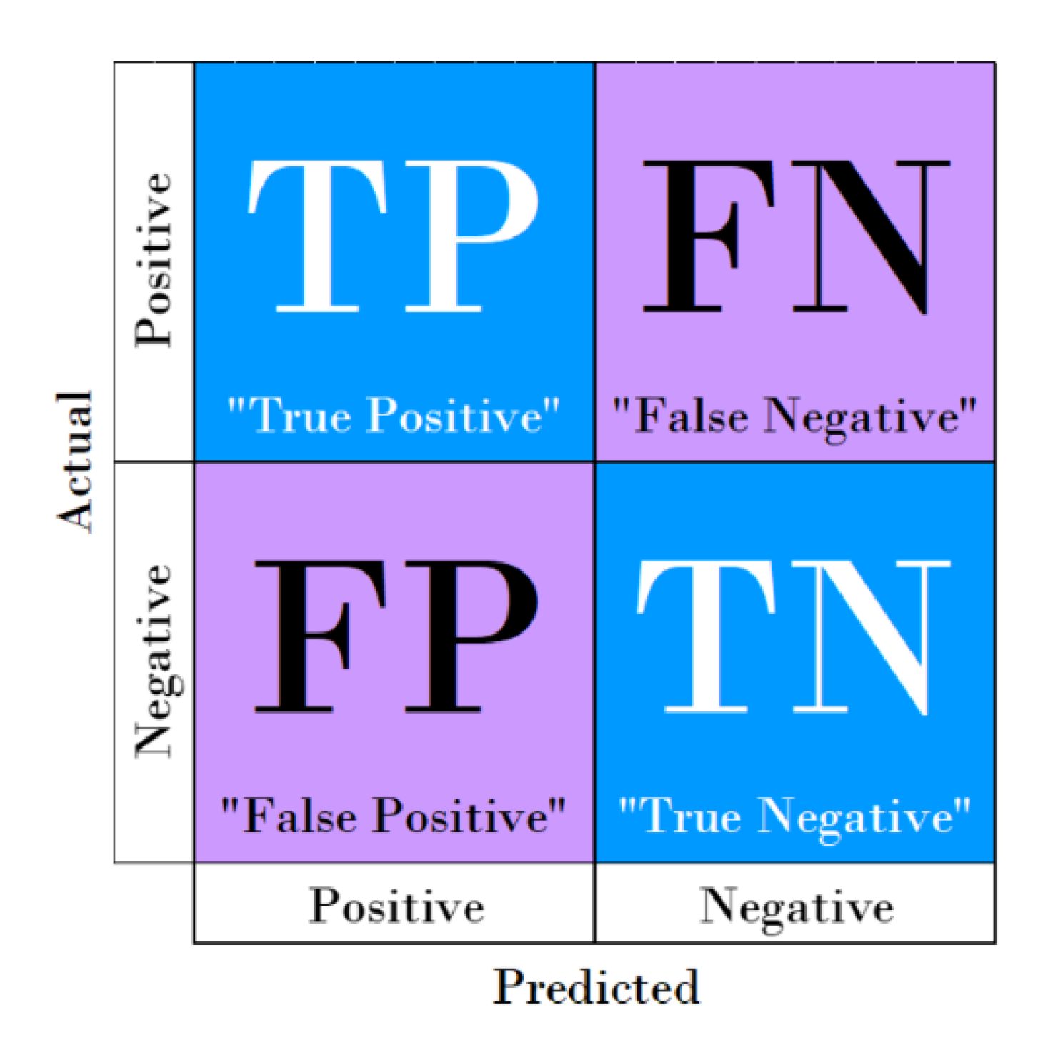
Regarding the prediction quality of classification models, it is first necessary to remind the reader that in a binary classification problem, samples are labeled as positive and negative so that evaluation metrics can be computed through the confusion matrix. The latter is a representation of the model’s classification accuracy, since it makes clear whether the system is mislabeling one class with another: each row of the confusion matrix represents the instances in an actual class, whereas each column represents those in a predicted class. Thus, the number of “true positives” (correctly classified positives), “true negatives” (correctly classified negatives), “false positives” (actual negatives classified incorrectly), and “false negatives” (actual positives classified incorrectly) can be defined. For a better understanding, a schematic representation of the confusion matrix is shown in
Figure 7.
To properly evaluate the TAdv classification model, samples in the “collision course” class have been labeled as positives. Thus, the recall (column 5,
Table 2) of the GRU
TADV model, representing the proportion of actual positive samples classified correctly, proves that the system is able to predict very accurately (values are greater than 0.870) whether the V2P interaction is moving or not moving on a collision course, whatever the prediction time-frame (despite the slight worsening discussed previously). Similarly, the AUC values (last column of
Table 2), greater than 0.995 at each time horizon, confirm the high accuracy of the binary classifier. Differently,
Figure 5 shows the effect of data distribution variability over the folds by ROC curves: as the time window gets longer, differences between folds are more evident, i.e., data distribution becomes sparser, and the model loses slightly in generalization capability. However, the performance is still more than acceptable.
For the S-GRU
SL model and the combined M-GRU
SL model, samples within the “unsafe” severity class have been labeled as positives. In the following, since the AUC calculation for a model that results from the combination of two GRU subsystems cannot be performed, the comparison between Approaches (1) and (2) is mainly based on accuracy and recall metrics (columns 3 and 5 of
Table 3). Analysis of results on the test set shows an improved ability of the S-GRU
SL model to label serious conflict interactions in near-accident events, especially over longer prediction timeframes. The accuracy of the S-GRU
SL model, i.e., the proportion of samples (positive and negative) classified correctly among all samples, is always higher than 0.970 on each timescale in contrast to the M-GRU
SL model, which only on the shortest time frame (1 s) reaches the value of 0.971. The situation gets even worse for the M-GRU
SL model to the advantage of the S-GRU
SL model in terms of recall (columns 5,
Table 3). In fact, the percentage gain in recall score (+15.40%, fourth column of
Table 4) by moving from the M-GRU
SL to S-GRU
SL model is noteworthy.
These results show that the combined model, due to the nonlinear error propagation from the single models (GRU
T2 and GRU
TADV), fails to generalize satisfactorily (as also evidenced by the standard deviations over folds) and performs significantly lower than S-GRU
SL. This finding is not trivial since, in many multi-step-ahead prediction problems, complex models (e.g., multiple GRUs) have performed better than equivalent simple models, such as a single GRU [
9].
In conclusion, despite the good results obtained in individual modeling of the T
2 and TAdv safety parameters, the S-GRU
SL model achieved the best performance, with an accuracy of 0.980, recall of 0.899 and AUC of 0.996 (averaged over the time windows and folds,
Table 4) in predicting near-accidental events of V2P encounters.


 ,
, 


