Effectiveness of Green Infrastructure Location Based on a Social Well-Being Index

Abstract

Urban Green Infrastructure (GI) provides promising opportunities to address today’s pressing issues in cities, mainly resulting from uncurbed urbanization. GI has the potential to make significant contributions to make cities more sustainable by satisfying the growing appetite for higher standards of living as well as helping cities adapt to extreme climate events. To leverage the potentials of GI, this article aims to investigate the effectiveness of GI that can enhance social welfare benefits in the triple-bottom line of urban sustainability. First, publicly available data sets representing social demographic, climate, and built environmental elements are collected and indexed to normalize its different scales by the elements, which is termed as the “Social Well-being Index.” Second, a random forest regressor was applied to identify the impacts of variables on the indexed scores by region. As a result, both the Seoul and Gyeonggi-do models found the most significant relationship with the type of GI to prevent pollutants and disasters, followed by GI types to conserve and improve the environment in Seoul and GI types to serve activity spaces in Gyeonggi-do. Furthermore, variables such as population, number of pollutants, and employment rate in Seoul were found significant and employment rate, population, and air pollution were significant in Gyeonggi-do. Finally, a scenario analysis is conducted to investigate the impacts of the overall index score with additional GI facilitation according to the model’s findings. This article can provide effective strategies for implementing policies about GI by considering regional conditions. The analytical processes in this article can provide useful insights into preparing effective ecological and environmental improvement policies accordingly.

1. Introduction

As humans settle together in cities, economies of scale and efficiency have been enhanced to better provide the essentials of residents. This has made our modern cities more attractive places to live and work because they offer higher living standards compared to rural areas [1]. In general, human society essentially requires resources and energy provided by nature; however, many human behaviors in cities treat these natural resources as free and almost unlimited. For the sake of living well, human society has built many built infrastructures—also known as grey infrastructure—and it has generated other challenges we have to face in cities [2].

Cities now face numerous societal and environmental challenges, such as inequity, resource depletion, climate changes, and air quality. These recent challenges are inextricably interconnected to the challenges we have faced in the past—e.g., rapid urban population growth, pollution, limited urban infrastructure networks. To mitigate these challenges, a series of urban renaissance projects (e.g., urban retrofitting, urban regeneration) are initiated to make cities more sustainable and livable areas. For example, urban renaissance projects [3,4] aim to meet policy objectives to enhance living standards (e.g., health, social cohesion), revitalize the local economy, and help cities adapt to climate changes.

As one of the promising solutions to a series of urban renaissance projects, approaches using Green Infrastructure (GI) are being discussed and understanding of GI’s potential has gained particular interests recently. Specifically, GI helps to avoid investing in a large-scale infrastructure system that requires enormous government budgets since it can often find cheaper and more durable solutions, generating various benefits. The European Commission (EU) [5], for instance, describes that the Green Space, an urban environmental indicator, is a nature-based solution that has been successfully tested in urban spaces, providing economic, social, and ecological benefits to sustainable development goals (SDGs) [6,7,8]. In general, GI is integrated into, or embedded within, other urban infrastructure systems to alleviate various challenges—e.g., stormwater management, carbon mitigation, energy savings in other infrastructure, air quality improvement, human health and well-being, and other social and ecological benefits. Moreover, since urban infrastructure and its consumption behaviors are intricately interconnected, GI can provide complementary solutions to existing grey infrastructure systems [2]. Therefore, GI has the potential to make significant contributions to making cities more sustainable by satisfying the growing appetite for higher standards of living as well as helping cities achieve a goal of urban sustainability.

GI holds many definitions and interpretations for different disciplines. From a planning and engineering perspective, in the realm of urban studies, it can be defined as strategically built or planned interconnected features with other infrastructure systems and environments, which can deliver a wide range of benefits to urban sustainability [9]. Several studies have concluded that whole or partially nature-based solutions, including GI and its associated elements, offer a wide range of benefits such as environmental, human health, and well-being (e.g., satisfaction) benefits in cities [1,5,10]. In terms of livability in cities, GI has various positive impacts on cities and residents [11]. The U.S. Environmental Protection Agency (EPA), for example, has also made various efforts to reduce the heat island effect in cities with vegetation, improving air quality and eliminating pollutants [12]. To put it differently, the rare integration of GI with cities has a negative impact on environmental ecosystems and the health and well-being of residents [13,14]. Based on the previous studies, it is obvious that the environmental and ecological improvements using GI can enhance residents’ overall conditions. In particular, it can be viewed that the importance of GI has a wide range of effects, from the psychological satisfaction of humans to environmental health. Therefore, securing sufficient GI has a positive impact on the satisfaction of the residents of urban environments.

In addition, previous studies also found that optimal implementation of GI can be an effective strategy for challenging issues in cities—e.g., water resources depletion, air quality issues, and other extreme events associated with climate change [15]. For instance, GI can improve air quality [16] and mitigate the heat island effect in the city center [17]. Providing that GI is sufficiently installed, extreme stormwater events, heat island effects, and air pollution can be alleviated [18]. More precisely, the effectiveness of GI largely depends on the location of GI being effectively integrated into, or embedded within, other urban infrastructure systems. In particular, some studies discuss the location of green spaces and GI while considering air pollution, noise, population, temperature, and green levels [19,20,21]. For example, Maruani and Amit-Cohen compared open space planning models to find effective factors. They concluded that both open space factors and external factors affect planning qualities [22]. Thompson suggested new patterns of connected open space to be effective with considerations of the size, application cost, period, complexity, etc. [23] Schilling and Logan suggested a model to find right sizes of GI by community sizes [24]. Votsis and BenDor et al. [10,25] found the impact of green areas on residential selection and child-rearing were found to be highly utilizable and efficient. Kim and Tran evaluated GI’s comprehensive plan performance in the United States and proposed a more comprehensive and concrete policy framework for local planners proposed for GI locations [26]. Campagnaro et al. [27] predicted the Pielou’s equivalence index of Green information from Italy’s Padua region, compared regional distributions according to variables, and discussed its applicability to find adequate locations. Lee and Oh [28] developed the GI location assessment system based on geographical information for Namyangju-si, Korea, and attempted the landscape ecological evaluation from both macro and micro perspectives. Zhou and Wu [29] attempted to distribute the Green Land of Hekou City, China, by matching the demand for rust and topographical characteristics. Lai et al. [30] identified the relationship between land use and spatial identification by presenting a plan to implement GIs in three areas near Cagliari, Italy.

In this circumstance, being able to analyze the effectiveness of GI is essential for municipalities and utilities to effectively meet users’ needs in urban areas. In particular, GI generally occupies large lots and has difficulty changing land use once implemented [17,31], thus, disproportionately distributed GI occurs potential degradation in ecological and environmental services [32,33,34]. Although some previous studies include fine-grained quantitative and qualitative information about GI for analyzing the impacts of GI, it is not applicable to most cities and municipalities where cities and utilities have limited access to the fine-grained data. Therefore, in this study, we suggest an approach to help policy makers and planning experts find a more feasible solution for determining the location of GI. Basically, the aim is to investigate the effectiveness of GI in urban areas that can enhance social welfare benefits for the triple-bottom line of urban sustainability to leverage the potential of GI. Furthermore, considering the connectivity aspects of the cities, maximizing the impacts of GI by allowing it to be linked to adjacent regions under the given conditions has been determined to have a more sustainable development direction. In addition, regional differences by functional and developmental characteristics by the linkage of population expansion and urban facilities will be considered. The specific objectives of this article are to answer the following research questions:

-

How does GI influence residents’ satisfaction with livability?

-

Which attributes of sociodemographic and regional characteristics are most sensitive for adopting GI?

-

How do we maximize the model’s application in the realm of urban studies?

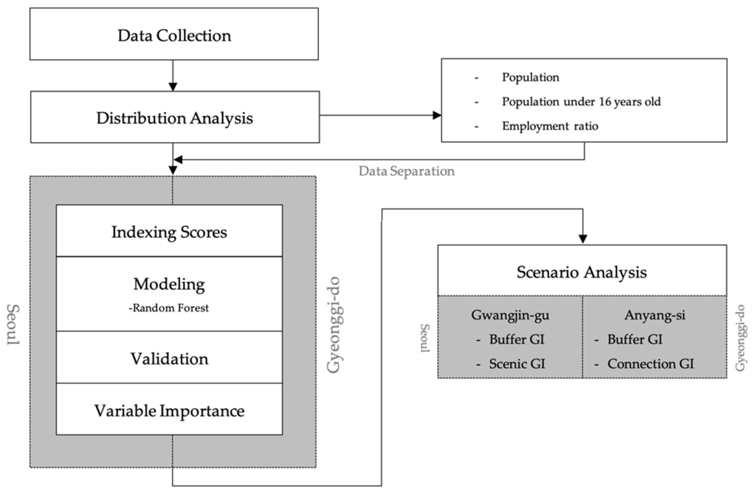
2. Materials and Method

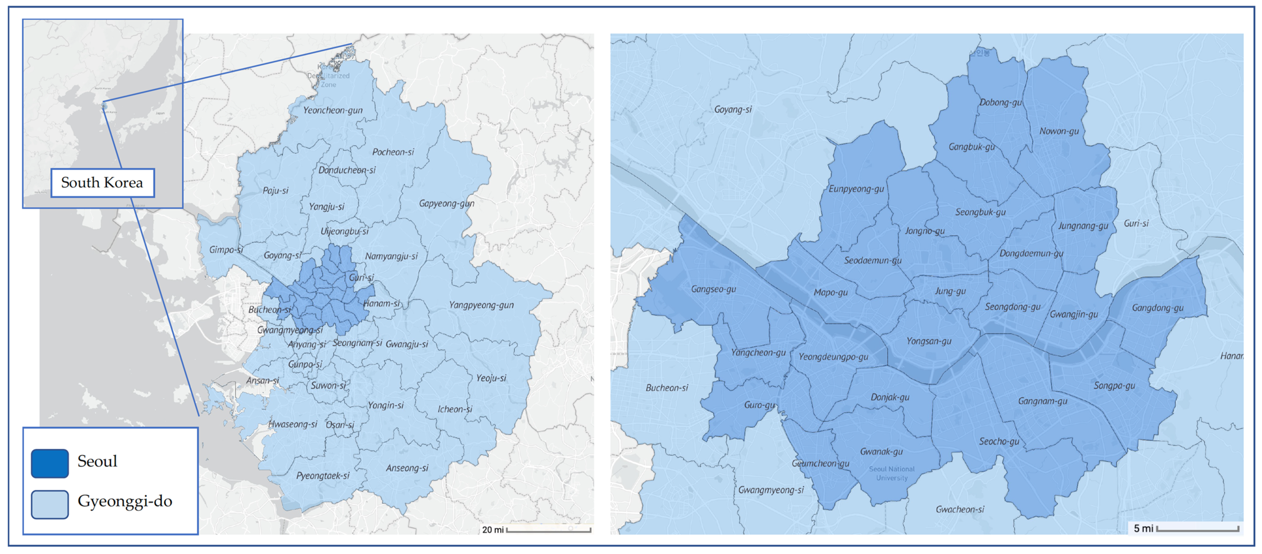
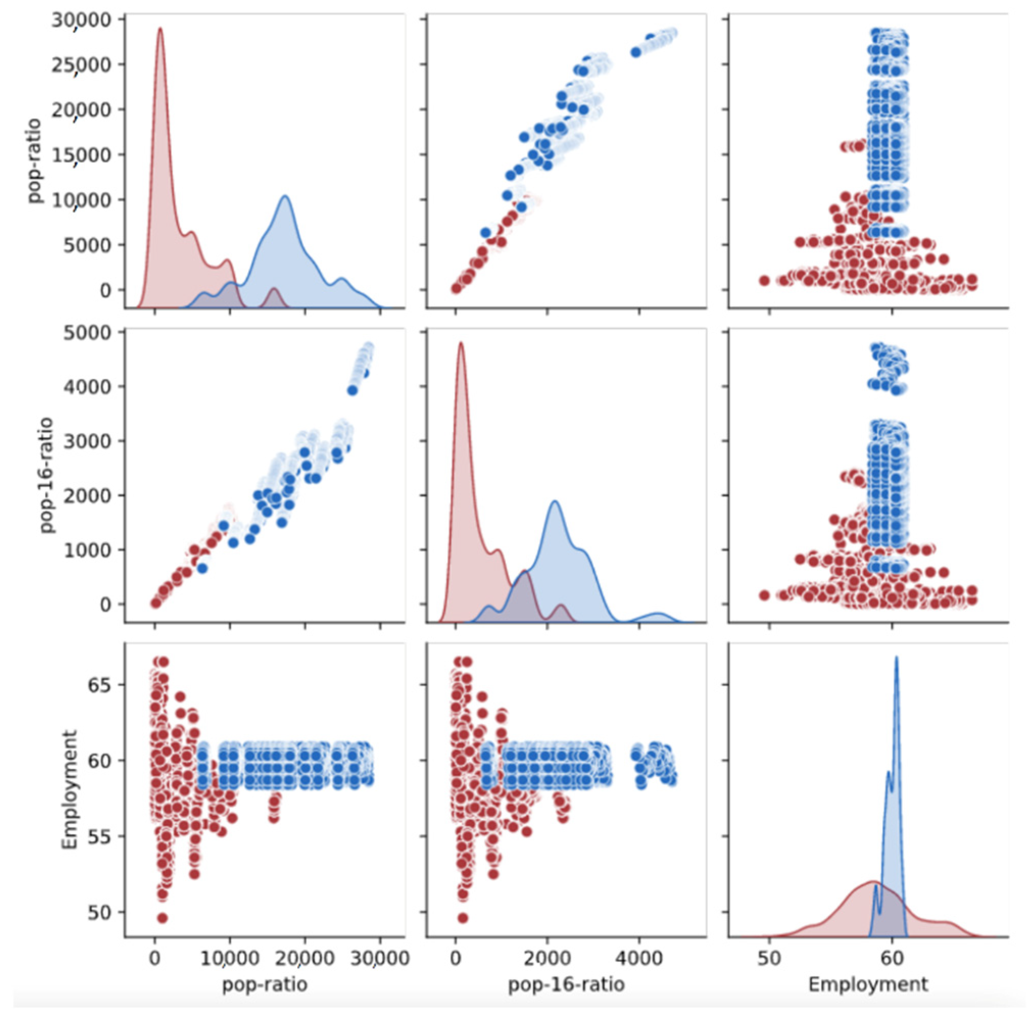
2.1. Materials

The overall research framework is described in Figure 1. Considering the geographical perspective of the research area, there are substantial distributional discrepancies between the two regions of Seoul and Gyeonggi-do. Thus, we made two different models to minimize technical issues in modeling—e.g., heterogeneity. To analyze the GI’s influence to their residents in two different regions, we adopt a random forest (RF) regressor, which is less susceptible to scales and outliers than other machine learning (ML) approaches [35,36,37]. Then, the estimated ML models are interpreted by surrogate interpretation techniques. Lastly, two scenario analyses were conducted to demonstrate the applicability of our models for future policy analysis.

This study geographically focused on 25 districts in Seoul and 31 cities and counties in Gyeonggi-do, as shown in Figure 2. In terms of high population concentration and interconnected facilities, residents’ responses to local GI changes were expected to be sensitive within the same living zone spectrum, thus ideal for evaluating alternatives to location green facilities presented in this work. In addition, through the relationship between better environmental conditions and population concentration, population and environmental variables are found to be highly interconnected throughout the research area, and the data should be available from the same sources to match. For reference, the detailed administrative district units of Seoul and Gyeonggi-do were marked as ‘area’ to represent them as unified terms in describing the data and the model setting and analysis stages.

Studies on location selection for balanced GI expansion in cities have been mainly done through micro-level optimization approaches through multi-objective optimization by setting specific environmental factors—for example, air quality, noise, population, temperature, green scale—as variables [18,38,39,40,41]. However, the implementation of GI’s facilities is characterized by having to override other projects in their location or size. It should consider a broader geographic area, including its vicinity, not just for the benefit of the region, which is the reason to provide information to consider the GI’s location at a higher level of the planning process to plan GI location preferentially [22]. In addition, various and ever-changing environmental factors should be included as much as possible to be analyzed in more detail.

Among the publicly available sources, data of demographics, GI, climate, and built environmental characteristics were collected, which can be used to check the environmental and ecological conditions of each region and area. To capture the concentration of the population in the city and its relationship or preference with climate and environmental variables in consideration of the population per unit area in each region, the area’s total numbers of the population, population under 16 years of age, and the employment ratio was considered. The annual data of GI, road rate, and the number of pollutants producing facilities were utilized as they were found to have an ecological impact on the urban environment. Green areas and the number of air pollution and water pollution emission facilities per area unit were considered. The Buffer GI is created to prevent pollution and natural disasters. The Connection GI serves as a walking space for urban residents by organically connecting parks, rivers, and mountainous areas. The Scenic GI is installed for environmental conservation and improvement. The three types of green areas are divided into Buffer GI, Connected GI, and Scenic GI by laws and regulations of the Ministry of Land, Infrastructure and Transport, the Ministry of Environment, and local governments. Since the scale of installation for each type of green area is also different, all three types of GIs were considered as variables differently in this study.

The climate variables were taken into account by the average monthly temperature (in Celsius), wind speed (meter/second), and rainfall (millimeter). The most stable air pollutants were collected using PM10 (Particulate Matter, finer than 10 micrometers) average monthly data (microgram/m²). The number of air and water pollution emission facilities for each area were collected. Considering the conventional time zone of the entire data, the time range was set from January 2013 to December 2019. The variables and their descriptive statistics are shown in

Table 1. Descriptive statistics of independent variables.

Variables	Description	Time Range	Mean	S.D.	Min.	Max.
Demographic characteristics
Pop	Total population	Year	404,873.60	252,774.03	43,824	1,203,285
Pop_16	Number of the population age 16 or under	Year	61,644.73	43,861.39	5020	213,391
Emp	Employment ratio (employed/total population)	Year	59.31	2.37	49.6	66.5
Green Infrastructure characteristics
Buffer_gi	Buffer Green Infrastructure area (m2)	Year	573,978.77	815,943.75	0	4,504,737
Scenic_gi	Scenic Green Infrastructure area (m2)	Year	494,455.95	2,672,348.84	0	34,908,592
Connection_gi	Connection Green Infrastructure area (m2)	Year	93,391.83	427,795.86	0	3,939,590
Built environment characteristics
Water_pol_fac	Number of water pollution facilities	Year	320.99	409.81	19	2775
Air_pol_fac	Number of air pollution facilities	Year	314.86	530.14	2	3231
Road	Road coverage (km2)	Year	11.65	10.21	0.11	28.83
Climate characteristics
temp	Temperature (°C)	Month	12.51	10.12	−8.5	29.3
wind	Wind speed (m/s)	Month	1.54	0.58	0	6.8
precipitation	Precipitation (mm/day)	Month	85.07	108.34	0	1076.50
PM10	Particulate Matters (<10 micrometers, micrograms/m2)	Month	47.39	15.81	6	124

.

Although there is no significant difference between weather and air pollution as Gyeonggi-do shares the same geographical characteristics with the boundary of the form surrounding Seoul as shown in Figure 1, it should be considered that there is a difference in the development process of the two regions [40].

To compare heterogeneous demographic characteristics between Seoul and Gyeonggi-do, bivariate probabilistic density for the two regions was estimated. Joint probability density estimation offers a means to study the joint probability density distribution between two variables (i.e., bivariate distribution) in a nonparametric way. This is significant because the joint probability density distribution between two variables captures the relationships between the two variables. In other words, it shows the probability by which each of the two variables falls in any certain intervals or discrete sets of values. For instance, suppose that $X$ and $Y$ are continuous variables, and $X$ takes values in $\left[a,b\right]$ and $Y$ takes values in $\left[c,d\right]$. Then the pair of $X$ and $Y$ takes the product $\left[a,b\right]\times \left[c,d\right]$. In this case, we can express the joint probability distribution of two variables, $X$ and $Y$, as:

$${\int }_c^d{\int }_a^{b}f\left(x,y\right)dxdy=1$$

(1)

In addition to studying the joint probability density distribution of two variables, we estimate a univariate probability density function for each single variable. Specifically, the univariate probability density function of a single variable, $X$, can be estimated using a kernel density estimation method. For instance, the estimated function ($\acute{f})$ for the variable, $X=\left\{x_1,x_2,\cdots x_n\right\}$, is derived from the kernel density estimator as defined below:

$$\acute{f_{\left(h\right)}}\left(x\right)=\frac{1}{n}\sum _{i=1}^n{K}_h\left(x-x_i\right)=\frac{1}{nh}\sum _{i=1}^{n}K(\frac{x-x_i}{h})$$

(2)

where $K$ is the kernel or weight function (it should be a non-negative function that integrates into one), and $h$ is a smoothing parameter that acts as a bandwidth. For the kernel ($K$) and the smoothing parameter ($h)$, we apply the standard normal kernel and auto-selection algorithm derived from the asymptotic mean integrated squared error (AMISE). In Figure 3, the bivariate probability distribution of demographic variables for the two regions was estimated.

The total population and the number of people under the age of 16 per unit area were clearly different in Seoul and Gyeonggi-do, and the comparison of employment rates showed that Seoul was concentrated in the 60% range, while Gyeonggi-do was widely spread around the late 50%. In terms of road rate, it was also confirmed that the road rate per unit area in Seoul was much higher than that of Gyeonggi-do. The relationship between the variables in Seoul and Gyeonggi-do were distributed and noticeably distinguishable from the difference between the characteristics of the two areas. Therefore, since it is reasonably concluded to consider the location of GI by the characteristics between the two regions, separate models were prepared.

2.2. Model Method

The selected and collected measurement data have different characteristics to compare as they are and they have difficulty considering weights. The alternative approach to resolve this conflict is the indexing method for measuring Better Life Index in the Organisation for Economic Co-operation and Development (OECD) [41] and Seoul, Korea [42]. In this study, this indexing method was applied to normalize the scale in the relevant variables and to utilize the sum of the entire scale as an index for analysis. It was named the Social Well-Being Index. Through the RF Regression, the importance of variables affecting index were examined by specifying the sum of index obtained by month and region as dependent variables. Seoul and Gyeonggi-do, which were established as research areas, were composed of separate models because the distribution of population and geographical characteristics were not the same. The model was constructed using data from 2013 to 2017, and it was validated using data from 2018 and 2019. Based on these estimated models and the importance of identified variables, a scenario analysis was conducted varying regionally important GI in Seoul and Gyeonggi-do to determine how much improvement is made in the Social Well-Being index in each region. Although a direct model for GI is not suggested, it is considered a more effective method for sustainable planning because it measures the expected effects of the expansion of GI in situations where both climate and environmental variables are considered.

2.2.1. Social Well-Being Index

Indexing is the process of leveling the range of analysis and identifiable indicators among the variables that affect climate and environmental condition in this research context. Since it is impossible to directly compare the original values of the data to each other because all the variables for the observed climate and environmental indicators were measured at different levels and ranges, the level and scope of the measurement are identified for correct comparison. In this process, the method of equalizing the values of the data was applied to the Min-Max method used by the OECD and Seoul, Korea, and variables will have index scores based on the following Equation (3):

$$Positive Var. Index=\frac{x_i-min\left(x\right)}{max\left(x\right)-min\left(x\right)}$$

(3)

where $x \mathrm{represents}\mathrm{the}\mathrm{input}\mathrm{records} \left(x=x_1,x_2,\cdots ,x_n\right)$.

As a result of this Equation (3), the index value is located between 0 and 1 regardless of the unit and distribution of the corresponding variable origin values enables comparison between variables. However, if the characteristics of the variables that make up the data have a negative meaning, such as the values of the pollutant facilities, air quality, and road rates, the corresponding indicators were used as minus the original equivalence value as shown in the Equation (4):

$$Negative Var.Index=1-\frac{x_i-min\left(x\right)}{max\left(x\right)-min\left(x\right)}$$

(4)

The index scores for all variables were obtained, and Equation (5) represents the

$$Social Well-Being Index=\sum _{}^{}Positive Var. Inde{x}_i+\sum _{}^{}Negative Var. Inde{x}_j$$

(5)

This process cancels the scale difference of the variables, and sets the sum of them, the Social Well-Being Index score, as the model’s dependent variable. Through this, each variable was exploited to determine the impact and relationship on the overall index.

As aforementioned, we used the sociodemographic and geographical characteristics of Seoul and Gyeonggi-do and the correlation among variables for two regions presented in Figure 4. The population in Seoul is highly correlated with a population under 16, showing a correlation at 0.92, but it is seen as a normal relationship when viewed at the rate of population size. Weather-related factors including precipitation and temperature of PM10, where inverse index scale is proposed, were all are found to be in the correct relationship. The relationship between air pollution source facilities and water pollution source facilities is also seen as a proper relationship because one facility often releases air and water pollutants simultaneously. Similar correlation patterns in population, weather, and pollutant facilities can be found in Gyeonggi-do, just as in Seoul. However, the difference from the Seoul area is that the road rate shows a high inverse correlation compared to the number of people. Considering that the road rate is inversely proportional, the road rate is higher in places with a large total population and a large population under the age of 16 and is more correlated than in Seoul. Unlike Seoul, Gyeonggi-do has developed arterials before its residential area, and this is also a proper relationship because public transportation networks are also not closely connected compared to Seoul. The two regional differences are also distinct in the correlation between the population, land use, and variables in Seoul and Gyeonggi-do. Therefore, we can see that developing a model for each of the two regions is the correct analysis approach.

2.2.2. Random Forest Regressor: Rule-Based Bootstrap Aggregation

Tree- and rule-based models, being applied to both classification and regression problems, are nonparametric modeling methods (also known as machine learning, ML) [43,44]. This nonparametric additive model learns the nonlinear relationships between a set of predictors and corresponding targets based on specific splitting rules without predetermined assumptions—e.g., linearity.

In particular, a regression tree (also known as a decision tree regressor), for example, is constructure by recursively partitioning the predictor space (i.e., samples) into several homogeneous groups (also known as tree nodes), which ends up with terminal nodes.

The goal of regression trees is to find non-overlapping partitions ($R_j$) that minimize the overall sum squared errors, given by:

$$SSE=\sum _{j=1}^J\sum _{i\in R_j}(y_i-{\widehat{y}}_{R_j})$$

(6)

where ${\widehat{y}}_{R_j}$ is the average response of the training observations within the $j$th partition. A single tree model locally learns patterns, i.e., local learners, and then aggregates local learners as a hierarchical tree structure (i.e., additive learning).

Thanks to the logic of their estimation, i.e., the set of splitting rules used to partition the predictor space are provided with a hierarchical structure (i.e., a tree), tree-based models have relative competitiveness with the other modeling approaches for various reasons. First, tree models built on an additive and hierarchical learning algorithm have gained popularity because of their ability of recognizing the non-linear patterns (e.g., non-linear relationships) of input features, while providing a higher degree of interpretability [44]. Furthermore, tree models can effectively handle various types of variables in nature (e.g., continuous, categorical, sporadically missing values) but also estimate models without having enough observations compared to other ML approaches—e.g., artificial neural networks [35,44].

Nonetheless, models learned by single trees or rules (e.g., regression tree) have two acknowledged weaknesses compared to other supervised learning approaches: (1) instability of model estimation and (2) relatively low predictive performance compared to other ML models. Specifically, the hierarchy of variables seen in a regression tree can vary each time a tree is estimated. In general, to train a regression tree, a certain portion of the data is commonly used, and the remaining portion is kept to test the accuracy of the tree, which is known as the “hold out” method. Therefore, if a different portion of the data is used to generate another tree, the hierarchy of variables changes. As a result, fitting one single tree is not enough to validate a hierarchy of variables. In addition, the latter is due to the fact that local fitting processes (i.e., recursively partitioning sub-regions) can increase the variance of the overall tree structure, which causes higher prediction errors than other ML models—i.e., bias-variance trade-off [45].

To alleviate these weaknesses of single tree models, bagging or bootstrap aggregation techniques (also known as ensemble methods) can be applied to balance the overall bias and variable of models [35,45,46]. RF regressor is basically an aggregate of bootstrapped trees (i.e., tree estimators) with decorrelating processes: (1) each bootstrapped tree is based on a random sub-sample of the given observations, and (2) each partition within each bootstrapped tree is split by a random subset of predictors. Thanks to this decorrelating process, RF can provide an additional improvement over simple bagging algorithms by reducing the correlation among the collection of bagged trees. RF regressor predicts y given $x_i$ as follows:

$$y\left(x_i\right)={\widehat{f}}_{RF}^N\left(x_i\right)=\frac{1}{N}\sum _{b=1}^N{T}_b\left(x_i\right)$$

(7)

where $x_i$ is a vector of an independent variable, $T_b\left(x_i\right)$ represents a single regression tree grown by bootstrapped samples including a subset of variables, and $N$ represents the total number of trees.

2.2.3. Interpretation of ML Models

As mentioned above, RF tends to show high predictive performance thanks to its machine-based repetitive computation (also known as a bagging process) [47]. Nonetheless, high predictive performance (e.g., prediction accuracy) does not provide enough information to investigate the impact of policies and associated users’ behaviors, especially in the realm of urban studies. To enhance the applicability of ML, urban analytics with ML also require an understanding of how model makes a certain decision based on the given data samples.

In predictive modeling, the contribution of predictor variables can be varied. In general, a few variables have substantial impacts on the result. To obtain useful information about the relative contribution of each variable, the reduction in bias and variance is measured, which is referred to as the “Variable Importance” (VI) (also known as the feature importance).

The sum of squared residuals (SSR) can be defined as:

$$SSR=\sum _{c\in leaves \left(T\right)}^{}\sum _{i\in c}^{} {\left(y_i-y_c\right)}^2$$

(8)

where $i$ is an observation on leaf $c$, and $y_i$ is the predicted value of the dependent variable of observation $i$. $y_c$ is the actual value of the dependent variable of leaf $c$. The changes in SSR among the variables indicates the VI of $x_j$ and it can be calculated as follows:

$$V{I}_d\left(x_j\right)={\Delta }_d=SS{R}_d-\sum _i^{}SS{R}_i^d$$

(9)

where $d$ denotes a node, $i$ is the branch of node d, $SS{R}_d$ is a terminal node (i.e., leaf node), and $SS{R}_i^d$ is an internal node. For the entire tree model, the VI score for each variable can be expressed as follows, where $D$ is the total number of nodes:

$$VI\left(x_j\right)=\frac{{\sum }_{d=1}^{D}V{I}_d\left(x_j\right)}{n\_nodes}$$

(10)

In general, the VI scores are expressed with the standardized values—i.e., ranging from 0 to 1. For instance, the VI score becomes zero (i.e., $V{I}_d\left(x_j\right)=0)$ when a variable has no “contribution”. This interpretation can provide useful insights into planning, regulatory factors, and policy impacts in the realm of urban studies. The SHAP package was utilized to visualize VI scores more readable [48].

3. Model Results

Based on the data from 2013 to 2017, the Social Well-Being Indices of Seoul and Gyeonggi-do were estimated through the RF Regressor. A total of 13 variables were used to build the model, including Buffer GI, Connection GI, Scenic GI, water and air pollutants facilities, road rates, wind speed, temperature, precipitation, air quality, total population, the population under 16 years of age, and the employment rate. As a result of validating the model using data from 2018 and 2019, a comparison of the estimated values of the Social Well-Being Index for each region and the model’s prediction values are shown in Figure 5.

Figure 5 presents plots between the estimated Social Well-Being Index value and the modeled value of 2018 and 2019, with an R-squared of 0.97 for the Seoul model and 0.98 for the Gyeonggi-do model. The explained variance score for the Seoul model is 0.96 and is 0.98 for Gyeonggi-do model.

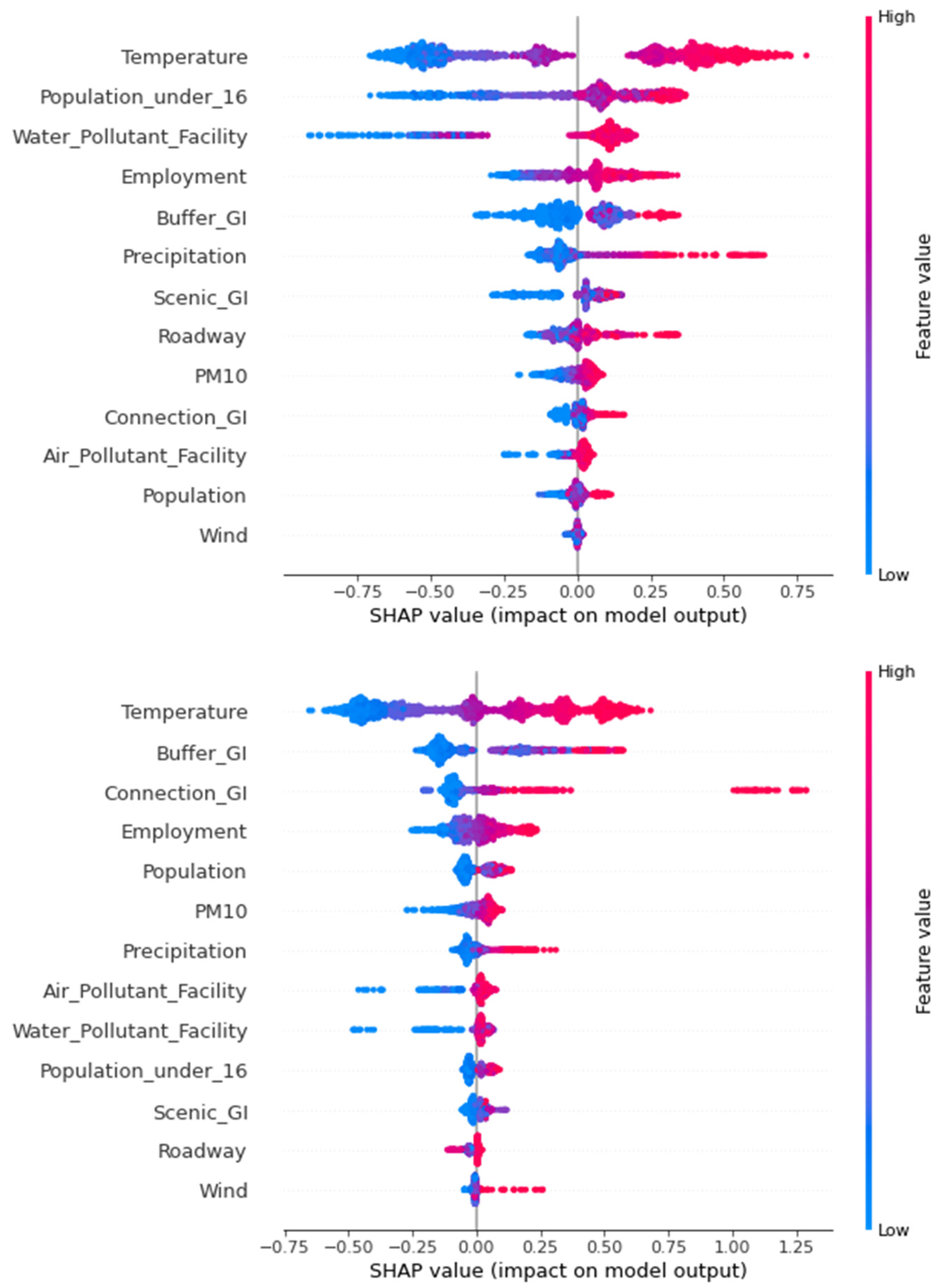
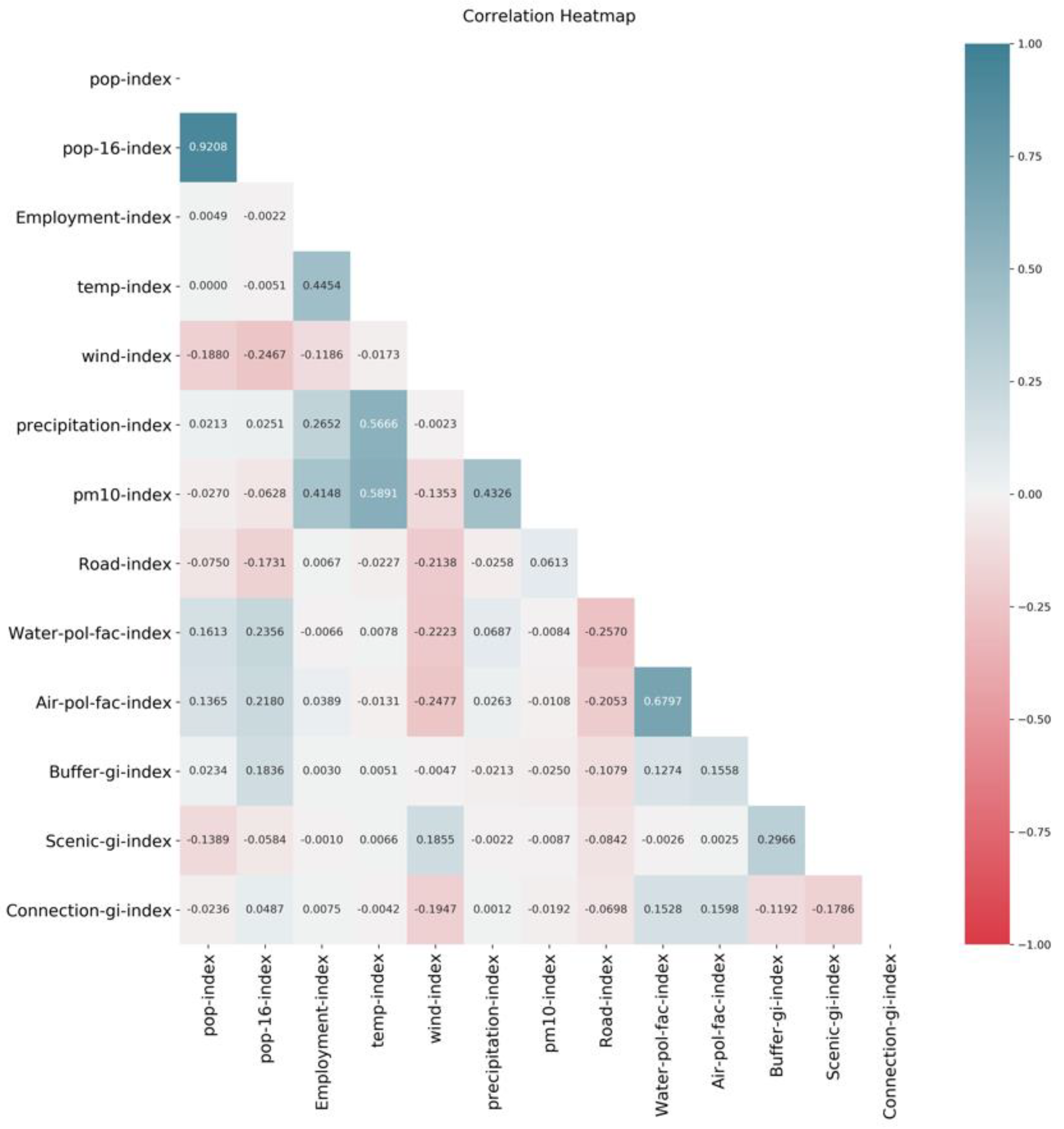
3.1. Relative Importance of Variable

In addition to the model’s high predictive accuracy, the VI is prepared to identify variables showing significant impacts on each model. As shown in Figure 6, the importance of the Seoul model was in the order of temperature, population under 16, water pollution source, employment, Buffer GI, precipitation, and Scenic GI, Gyeonggi-do model was in the order of temperature, Buffer GI, Connection GI, employment, population, PM10, and precipitation. It is interesting to see that the temperature in both regions has the most significant impact on the overall model prediction. Regarding GI, both the Seoul and Gyeonggi models were found to significantly impact the Buffer GI compared to other GI models. Due to the characteristics of Buffer GI, it was judged that the more it was installed to distinguish it from the contaminated or pollution emitting facility, the more it affected the entire index. Scenic GI seems to have a positive impact in the Seoul model because development has already been completed, and the concentration of residents in urban areas is high. However, the competition model showed higher importance of Connection GI connecting to green areas outside the city center, indicating that the shape of GI affecting the index was also different.

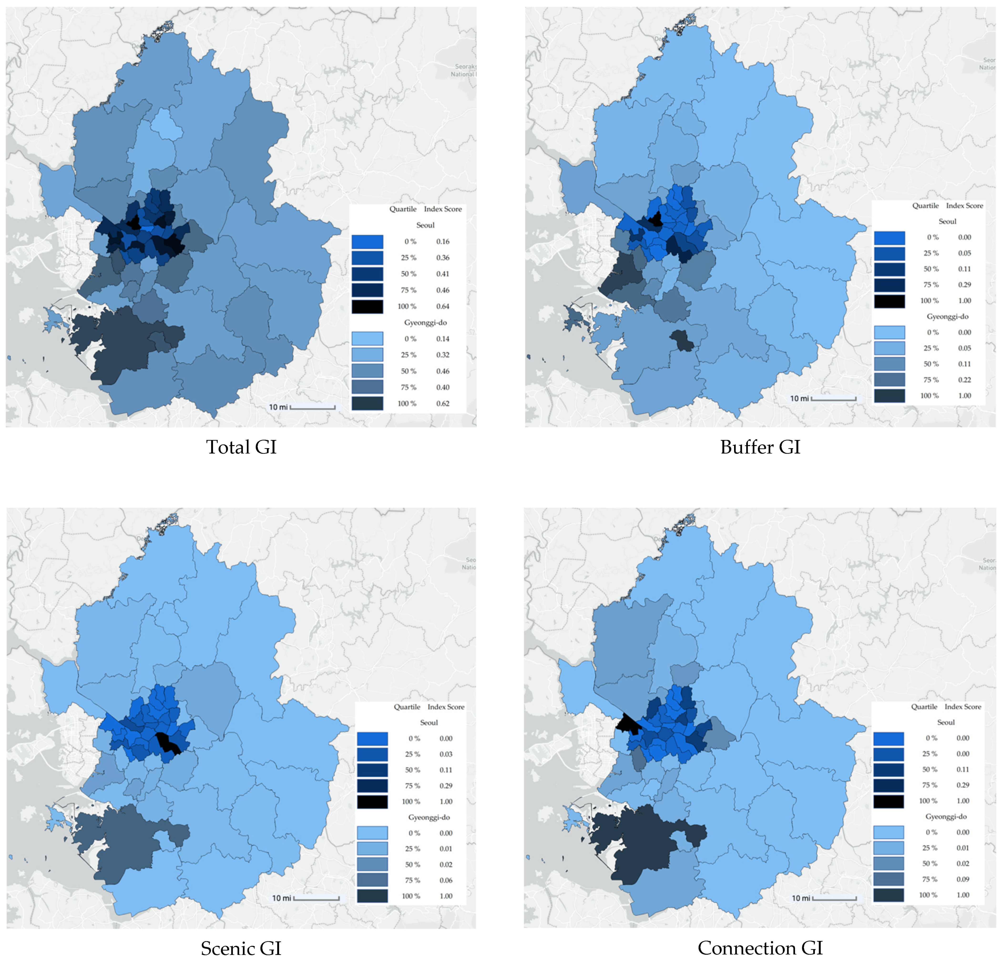
3.2. Green Infrastructure Index Distribution

A visual representation is prepared in Figure 7 with the total index by region and the index values by the shape of GI to identify differences in regional distributions.

Comparing the Social Well-Being Index scores, Seoul generally showed higher scores in most regions. On the other hand, Gyeonggi-do showed higher index scores in the south than in the north. It is easy to see that the index value of each GI varies from region to region. For example, the buffer GI was found installed in areas that include airports and major highways in Seoul. In contrast, Gyeonggi-do was found to represent high scores in areas near highways and industrial complexes entering Seoul. Connection GI obtained a high index score in some areas—i.e., the connection of green areas among parks. However, Scenic GI is in one of Seoul’s highest areas where a particularly high availability of space has been confirmed. In addition, various types of GI are sporadically distributed in Seoul. Still, in Gyeonggi-do, the distribution of GI is located adjacent to Seoul and more in the southern region than in the northern part.

4. Scenario Analysis and Discussion

4.1. Scenario Analysis: Potential Impacts of GI on Social Well-Being Index

As mentioned above, a model was designed to measure the Social Well-Being Index by using publicly accessible information, representing demographic, green infrastructure, climate, and built-environment characteristics. The models were verified by a 10-fold cross-validation process. Based on the estimated models, a scenario analysis was designed to further analyze the impacts of GI for the Social Well-Being index score. Specifically, the impacts of the Social Well-Being Index score resulted from the changes in the GI ratio were measured by selecting a specific area in each region. Climate conditions, including temperature, wind speed, precipitation, and demographic conditions, are assumed to be fixed. The scenario is established considering only the magnitude change of the GI types, the main object of this study. Too many combinations are expected for scenario analysis across the region, and the performance of model effects is not easy to observe. Therefore, each area with a low GI ratio and a high population ratio in Seoul and Gyeonggi-do was selected. The effect of the Social Well-Being Index on more residents when the area of GI is expanded by region is examined. As a result of checking the most recent record in the data, Gwangjin-gu in Seoul and Anyang-si in Gyeonggi-do were selected based on data from December 2019. Considering the differences in regional GI importance through the VI of RF regressor as shown in Figure 6, each scenario is prepared by adjusting the ratio of Buffer and Scenic GIs for Gwangjin-gu and adjusting the Buffer ratio Connection GIs for Anyang-si. The selected area’s GIs are set as the default outcome—Base Case—and three different scenarios are prepared: the mean of the region’s unit area, 150% of the mean, and the highest unit area. Therefore, Gwangjin-gu, Seoul, has set a scenario that applies Buffer GI and Scenic GI to Seoul’s mean, 150 percent of the mean, and the highest ratio in Seoul. Anyang-si, Gyeonggi-do, confirmed the change in Social Well-Being Index scores by setting up and applying Buffer GI and Connection GI three scenarios, which apply the mean, 150% of the mean, and the highest ratio in Gyeonggi-do.

The overall scenario design and analysis results can be found in

Table 2. Scenario variables and Social Well-being Index ranks.

Analysis Cases		GI Type	Gwangjin-gu (Seoul)		Anyang-si (Gyeonggi-do)
			Ratio	Index Rank	Ratio	Index Rank
Base case (December 2019)		Buffer	0.099%	10	0.551%	28
		Scenic	0.011%		0.219%
		Connection	0.000%		0.043%
Scenario cases	Mean ratio	Buffer	0.506%	9	0.520%	28
		Scenic	0.151%		0.219%
		Connection	0.000%		0.055%
	150% of the mean ratio	Buffer	0.759%	8	0.780%	26
		Scenic	0.226%		0.219%
		Connection	0.000%		0.083%
	Maximum ratio	Buffer	2.467%	1	1.969%	6
		Scenic	1.062%		0.219%
		Connection	0.000%		0.506%

and the Social Well-Being Index also improved as the proportion of GI increases. In the case of Gwangjin-gu, Seoul, the improvement of the Social Well-Being Index was confirmed in all three scenarios because the area ratios of Buffer and Scenic GI were observed to be lower than the average of Seoul and enough spaces for the GI was available for its Social Well-being index score improvements. Interestingly, due to the relatively low GI ratio compared to other districts in Seoul, the Index value represented the highest rank in the entire city as the GI area ratio increases. Anyang-si, Gyeonggi-do, can see that if Buffer and Connection GIs are adjusted to the mean of Gyeonggi-do, the ratio of Buffer GI was lower than the current one, and the ratio of Connection GI was higher than the present condition, resulting in no change due to the trade-off result in the overall Index values. Instead, when the GI area ratio is 150%, and the maximum of the mean of Gyeonggi-do, the rise of Social Well-Being Index rank resulted in being proportional to the increase in GI area ratio. In conclusion, when each area in Seoul and Gyeonggi-do was selected to analyze the scenario cases and scrutinize the results, the changes and predictions in the model do not deviate significantly from the previous verification results and are confirmed to be reliable. In addition, rather than randomly increasing the proportion of GI, the Social Well-Being Index can significantly promote the efficiency of GI positioning and sizing and maximize its effectiveness. Residents’ livability can be increased in the process of presenting a location to install GI that can achieve the appropriate size and a high efficiency, and it will be a valuable reference in the policy-making process. Finally, upon this process being undertaken appropriately, the burden of post-GI location changes will be alleviated, enabling more active policy implementation and sustaining policy direction to maintain viability through proper form of GI installation in line with long-term land use development.

4.2. Discussion

This article aims to investigate the impacts of GI and the relevant factors affecting life satisfaction in cities by adopting ML approaches (i.e., random forest regressor) with surrogate interpretation. Specifically, the model is designed to investigate an index score of variables for various characteristics and scales, suggesting the analytical potential to represent the overall well-being state of the city and the availability of GI location choices in a sustainable urban space. Existing GI studies mainly considered geographic and topographic characteristics as key variables [26,27,28,29,30]. In this study, however, publicly accessible descriptive variables—i.e., demographic, climate, environment, and form-specific GI variables—were considered together to enable the overall efficiency improvement of urban elements, including residents. This revealed that the variables utilized in the model and Social Well-Being Index have different regional relationships and confirmed that the different GI types are found important in the models. Further scenario analysis allowed us to verify the effectiveness of improving Social Well-Being Index efficiently when expanding GIs that we considered to be regionally important. In this context, it is possible to choose a location for GI that increases equity with the surrounding regions and indicated that it was effective in establishing sustainable development plans for planners.

In addition, the findings from this article can help planners consider and evaluate efficient and proper location of the GIs in the Social Well-being perspectives. The results of the study suggested that effective location selection of GIs is also effective across urban areas. Recently, research on the effectiveness and location of GIs has been highly interested in, and efforts have been made to apply them to planning processes through various approaches. In addition, as various data become available, models that take many variables into account are presented and the application feasibility is emphasized through case examples. However, we believe that the model that does not consider residents and their circumstances, the largest and essential beneficiaries of GI, deviates from the core of sustainable development in urban areas where new natural GI cannot be found. Selecting a location in consideration of the type of household composition of residents, employment conditions, road accessibility, and climate and environmental factors in their lives can secure the sustainability of existing and new GI in cities. Residents’ livability can be increased in the process of presenting a location to install GI that can achieve appropriate size and high efficiency, and it will be a valuable reference in the policy-making process. Finally, upon this process being undertaken appropriately, the burden of post-GI location changes will be alleviated, enabling more active policy implementation and sustaining policy direction to maintain viability through proper form of GI installation in line with long-term land use development.

Lastly, predictive models have been integral for urban infrastructure planning as well as decision-making process in urban contexts to investigate urban behaviors and phenomena. Nonetheless, researchers generally face technical challenges when analyzing real-world urban problems, such as the availability of data and modeling techniques. Although we are living in the era of Big Data, most cities and utilities generally do not have access to fine-grained information about the characteristics of urban areas. In this context, this article can provide useful insights into constructing acceptable models using publicly accessible descriptive variables for understanding the relationship between users’ satisfaction and GI systems in an urban context.

5. Conclusions

In this study, data on climate and environmental factors as well as demographics and pollutant facilities were quantified through indexing before the RF regressor was used to identify GI’s ecological and environmental factors to present more objective evaluation criteria in selecting GI locations. As a result of the models for Seoul and Gyeonggi-do, by GI types, both models have the largest impact by Buffer GI, followed by Scenic GI in Seoul and Connection GI in Gyeonggi-do. In addition, variables such as population, number of pollutants, and employment rate in Seoul were found significant, and Gyeonggi-do had a big impact on employment rate, population, and air pollution. As a result, the improvement of the overall index score was identified, indicating a noticeable improvement in the Ecological Index (see Figure 7).

Based on the data and analysis results, it was possible to identify efficient GI installation conditions by region and present criteria to maximize GI installation effectiveness based on climate and environmental improvement policies. It is also noteworthy that this research has identified the possibility of a local Social Well-Being Index to analyze utilizing existing measurements and collection data, rather than requiring additional and more resources to check the weights of variables. The three issues promised in the introduction of the study were also identified: (1) how GI affects residents’ satisfaction; (2) what variables are most sensitive to GI installation; and (3) how to maximize the actual application of the model. The index score was calculated to measure social well-being standards and the model predicted their major impacts. The GI variables were found to be significant among all and the significance was different by Seoul and Gyeonggi-do. Sensitive variables associated with GI installation were demographic variables, and additional needs were identified according to the existing GI installation level. Scenario analysis also highlighted that the practical applicability of urban research and concluded the ML-based model showed impressively high predictive accuracy and identified the region’s characteristics by establishing a distinguished model of Seoul and Gyeonggi-do from the inconsistent distribution characteristics of regional data. It is encouraging that such built models are also sensitive in real-case scenario analysis, confirming the potential to help decision makers make policy decisions. However, there is still a possibility of expansion in collecting extensive data considering the diverse variables of urban context including ecologic and environmental variables, time range, and transferability of the model prepared for the Social Well-Being Index. Furthermore, it is expected that more efficient GI location exploration will be possible through a comprehensive model construction that considers these variables. Finally, detailed standards for urban development and facility preparation can be provided if a more detailed model is estimated according to the applied classification rather than the type of GI.

References

1. Allen Klaiber, H.; Phaneuf, D.J. Valuing Open Space in a Residential Sorting Model of the Twin Cities. J. Environ. Econ. Manag. 2010, 60, 57–77. [Google Scholar] [CrossRef]
2. Pauleit, S.; Ambrose-Oji, B.; Andersson, E.; Anton, B.; Buijs, A.; Haase, D.; Elands, B.; Hansen, R.; Kowarik, I.; Kronenberg, J.; et al. Advancing Urban Green Infrastructure in Europe: Outcomes and Reflections from the GREEN SURGE Project. Urban For. Urban Green. 2019, 40, 4–16. [Google Scholar] [CrossRef]
3. Department for Transportation, Local Government and the Regions. Towards an Urban Renaissance; Taylor & Francis: Abingdon, UK, 1999. [Google Scholar]
4. Imrie, R.; Raco, M. Urban Renaissance—New Labour, Community, and Urban Policy; The Policy Press: Bristol, UK, 2003. [Google Scholar]
5. European Commission; Expert Group on the Urban Environment. European Sustainable Cities; Nuclear Safety and Civil Protection: Brussels, Belgium, 1996. [Google Scholar]
6. United Nations. The Sustainable Development Goals Report; The Department of Economic and Social Affairs: New York, NY, USA, 2020. [Google Scholar]
7. Department of Economics and Social Affairs. The Future Is Now—Science for Achieving Sustainable Development; United Nations: New York, NY, USA, 2019. [Google Scholar]
8. Derrible, S. Urban Engineering for Sustainability; The MIT Press: Cambridge, MA, USA, 2019; ISBN 978-0-262-04344-1. [Google Scholar]
9. City of Portland. Portland’s Green Infrastructure: Quantifying the Health, Energy and Community Livability Benefits; City of Portland: Portland, WA, USA, 2010; p. 101. [Google Scholar]
10. Votsis, A. Planning for Green Infrastructure: The Spatial Effects of Parks, Forests, and Fields on Helsinki’s Apartment Prices. Ecol. Econ. 2017, 132, 279–289. [Google Scholar] [CrossRef] [Green Version]
11. Botkin, D.B.; Beveridge, C.E. Cities as Environment. Urban Ecosyst. 1997, 1, 3–19. [Google Scholar] [CrossRef]
12. Sandström, U.G. Green Infrastructure Planning in Urban Sweden. Plan. Pract. Res. 2002, 17, 373–385. [Google Scholar] [CrossRef]
13. United States Environmental Protection Agency (US EPA). Benefits of Green Infrastructure; US EPA: Washington, DC, USA, 2021.
14. Tzoulas, K.; Korpela, K.; Venn, S.; Yli-Pelkonen, V.; Kaźmierczak, A.; Niemela, J.; James, P. Promoting Ecosystem and Human Health in Urban Areas Using Green Infrastructure: A Literature Review. Landsc. Urban Plan. 2007, 81, 167–178. [Google Scholar] [CrossRef] [Green Version]
15. Wu, J.; Plantinga, A.J. The Influence of Public Open Space on Urban Spatial Structure. J. Environ. Econ. Manag. 2003, 46, 288–309. [Google Scholar] [CrossRef]
16. Mell, I.C. Can Green Infrastructure Promote Urban Sustainability? Proc. Inst. Civ. Eng. Eng. Sustain. 2009, 162, 23–34. [Google Scholar] [CrossRef]
17. Sung, H.-C.; Hwang, S. A Preliminary Study on Assessment of Urban Parks and Green Zones of Ecological Attributes and Responsiveness to Climate Change. J. Korea Soc. Environ. Restor. Technol. 2013, 16, 107–117. [Google Scholar] [CrossRef]
18. Zhang, Y.; Murray, A.T.; Turner, B.L. Optimizing Green Space Locations to Reduce Daytime and Nighttime Urban Heat Island Effects in Phoenix, Arizona. Landsc. Urban Plan. 2017, 165, 162–171. [Google Scholar] [CrossRef]
19. Meerow, S.; Newell, J.P. Spatial Planning for Multifunctional Green Infrastructure: Growing Resilience in Detroit. Landsc. Urban Plan. 2017, 159, 62–75. [Google Scholar] [CrossRef]
20. Liu, Y.; Wang, R.; Grekousis, G.; Liu, Y.; Yuan, Y.; Li, Z. Neighbourhood Greenness and Mental Wellbeing in Guangzhou, China_ What Are the Pathways? Landsc. Urban Plan. 2019, 190, 9. [Google Scholar] [CrossRef]
21. Neema, M.N.; Ohgai, A. Multitype Green-Space Modeling for Urban Planning Using GA and GIS. Environ. Plan. B Plan. Des. 2013, 40, 447–473. [Google Scholar] [CrossRef]
22. Yuan, Z.; Tiemao, S.; Chang, G. Multi-Objective Optimal Location Planning of Urban Parks. In Proceedings of the 2011 International Conference on Electronics, Communications and Control (ICECC), Ningbo, China, 9–11 September 2011; pp. 918–921. [Google Scholar]
23. Maruani, T.; Amit-Cohen, I. Open Space Planning Models: A Review of Approaches and Methods. Landsc. Urban Plan. 2007, 81, 1–13. [Google Scholar] [CrossRef]
24. Thompson, C.W. Urban Open Space in the 21st Century. Landsc. Urban Plan. 2002, 60, 59–72. [Google Scholar] [CrossRef]
25. BenDor, T.; Westervelt, J.; Song, Y.; Sexton, J.O. Modeling Park Development through Regional Land Use Change Simulation. Land Use Policy 2013, 30, 1–12. [Google Scholar] [CrossRef]
26. Kim, H.; Tran, T. An Evaluation of Local Comprehensive Plans Toward Sustainable Green Infrastructure in US. Sustainability 2018, 10, 4143. [Google Scholar] [CrossRef] [Green Version]
27. Campagnaro, T.; Sitzia, T.; Cambria, V.E.; Semenzato, P. Indicators for the Planning and Management of Urban Green Spaces: A Focus on Public Areas in Padua, Italy. Sustainability 2019, 11, 7071. [Google Scholar] [CrossRef] [Green Version]
28. Lee, D.; Oh, K. The Green Infrastructure Assessment System (GIAS) and Its Applications for Urban Development and Management. Sustainability 2019, 11, 3798. [Google Scholar] [CrossRef] [Green Version]
29. Zhou, C.; Wu, Y. A Planning Support Tool for Layout Integral Optimization of Urban Blue–Green Infrastructure. Sustainability 2020, 12, 1613. [Google Scholar] [CrossRef] [Green Version]
30. Lai, S.; Leone, F.; Zoppi, C. Assessment of Municipal Masterplans Aimed at Identifying and Fostering Green Infrastructure: A Study Concerning Three Towns of the Metropolitan Area of Cagliari, Italy. Sustainability 2019, 11, 1470. [Google Scholar] [CrossRef] [Green Version]
31. Giles-Corti, B.; Broomhall, M.H.; Knuiman, M.; Collins, C.; Douglas, K.; Ng, K.; Lange, A.; Donovan, R.J. How Important Is Distance To, Attractiveness, and Size of Public Open Space? Am. J. Prev. Med. 2005, 28, 169–176. [Google Scholar] [CrossRef]
32. Liang, X.; Tian, H.; Li, X.; Huang, J.-L.; Clarke, K.C.; Yao, Y.; Guan, Q.; Hu, G. Modeling the Dynamics and Walking Accessibility of Urban Open Spaces under Various Policy Scenarios. Landsc. Urban Plan. 2021, 207, 103993. [Google Scholar] [CrossRef]
33. Chiesura, A. The Role of Urban Parks for the Sustainable City. Landsc. Urban Plan. 2004, 68, 129–138. [Google Scholar] [CrossRef]
34. Roe, M.; Mell, I. Negotiating Value and Priorities: Evaluating the Demands of Green Infrastructure Development. J. Environ. Plan. Manag. 2013, 56, 650–673. [Google Scholar] [CrossRef]
35. Lee, D.; Derrible, S. Predicting Residential Water Demand with Machine-Based Statistical Learning. J. Water Resour. Plan. Manag. 2020, 146, 04019067. [Google Scholar] [CrossRef]
36. Pedregosa, F.; Varoquaux, G.; Gramfort, A.; Michel, V.; Thirion, B.; Grisel, O.; Blondel, M.; Prettenhofer, P.; Weiss, R.; Dubourg, V.; et al. Scikit-Learn: Machine Learning in Python. JMLR 2011, 12, 2825–2830. [Google Scholar]
37. James, G.; Witten, D.; Hastie, T.; Tibshirani, R. An Introduction to Statistical Learning with Applications in R, 2nd ed.; Springer: Berlin/Heidelberg, Germany, 2013; Volume 112, ISBN 978-1-4614-7138-7. [Google Scholar]
38. Abhijith, K.V. Air Pollution Abatement Performances of Green Infrastructure in Open Road and Built-up Street Canyon Environments—A Review. Atmos. Environ. 2017, 162, 71–86. [Google Scholar] [CrossRef]
39. De Groot, R.S. Functions of Nature: Evaluation of Nature in Environmental Planning Management and Decision-Making; Wolters-Noordhoff BV: Toronto, ON, Canada, 1992; ISBN 90-01-35594-3. [Google Scholar]
40. Seoul Metropolitan Governments. Urban Planning-Seoul’s Unique, Sustainable Urban Planning; Seoul Solution: Seoul, Korea, 2021. [Google Scholar]
41. OECD. How’s Life in Your Region? Measuring Regional and Local Well-Being for Policy Making; OECD: Paris, France, 2014. [Google Scholar]
42. Byun, M.; Choi, J.; Park, M.; Lee, H. The Quality of Life in Megacity and Seoul-Specific Happiness Indicator; Seoul Research Institute: Seoul, Korea, 2015. [Google Scholar]
43. Bishop, C.M. Pattern Recognition and Machine Learning; Springer: New York, NY, USA, 2006; ISBN 978-0-387-31073-2. [Google Scholar]
44. Hastie, T.; Tibshirani, R.; Friedman, J. The Elements of Statistical Learning; Springer Series in Statistics; Springer: New York, NY, USA, 2009; ISBN 978-0-387-84858-7. [Google Scholar]
45. Lee, D.; Mulrow, J.; Haboucha, C.J.; Derrible, S.; Shiftan, Y. Attitudes on Autonomous Vehicle Adoption Using Interpretable Gradient Boosting Machine. Transp. Res. Rec. 2019, 2673, 865–878. [Google Scholar] [CrossRef]
46. Breiman, L. Random Forests. Mach. Learn. 2001, 45, 5–32. [Google Scholar] [CrossRef] [Green Version]
47. Friedman, J.H. Greedy Function Approximation: A Gradient Boosting Machine. Ann. Statist. 2001, 29. [Google Scholar] [CrossRef]
48. Lundberg, S.M.; Lee, S.-I. A Unified Approach to Interpreting Model Predictions. In Proceedings of the Advances in Neural Information Processing Systems; Guyon, I., Luxburg, U.V., Bengio, S., Wallach, H., Fergus, R., Vishwanathan, S., Garnett, R., Eds.; Curran Associates, Inc.: Red Hook, NY, USA, 2017; Volume 30, pp. 4765–4774. [Google Scholar]
Figure 1. Research design.
Sustainability 13 09620 g001
Figure 2. Geographical scope of the research area—Seoul and Gyeonggi-do in South Korea.
Sustainability 13 09620 g002
Figure 3. Demographic bivariate distribution for Seoul and Gyeonggi-do (Seoul in blue and Gyeonggi-do in red).
Sustainability 13 09620 g003
Figure 4. Correlation between variables in two regions (Relationship of positive in blue and negative in red; above: Seoul, below: Gyeonggi-do).
Sustainability 13 09620 g004aSustainability 13 09620 g004b
Figure 5. RF model performance plot (Left—Seoul, Right—Gyeonggi-do).
Sustainability 13 09620 g005
Figure 6. Importance of variables (Upper—Seoul, Lower—Gyeonggi-do).
Sustainability 13 09620 g006
Figure 7. Social Well-being Index score distribution.
Sustainability 13 09620 g007