Energy Distribution Modeling for Assessment and Optimal Distribution of Sustainable Energy for On-Grid Food, Energy, and Water Systems in Remote Microgrids

Abstract

Food, energy, and water (FEW) are essential for human health and economic development. FEW systems are inextricably interlinked, yet individualized and variable. Consequently, an accurate assessment must include all available and proposed FEW components and their interconnections and consider scale, location, and scope. Remote Alaska locations are examples of isolated communities with limited infrastructure, accessibility, and extreme climate conditions. The resulting challenges for FEW reliability and sustainability create opportunities to obtain practical insights that may apply to other remote communities facing similar challenges. By creating energy distribution models (EDMs), a methodology is proposed, and a tool is developed to measure the impacts of renewable energy (RE) on small FEW systems connected to the microgrids of several Alaska communities. Observing the community FEW systems through an energy lens, three indices are used to measure FEW security: Energy–Water (EW), Energy–Food (EF), and Sustainable Energy (SE). The results indicate the impacts of RE on FEW infrastructure systems are highly seasonal, primarily because of the natural intermittence and seasonality of renewable resources. Overall, there is a large potential for RE integration to increase FEW security as well as a need for additional analysis and methods to further improve the resiliency of FEW systems in remote communities.

1. Introduction

Food, energy, and water (FEW) are vital to human health and enable economic development. FEW systems are interconnected, calling for a comprehensive perspective. For example, energy is required to extract and supply potable water. Water, in turn, enables electricity generation in Rankine cycles or hydrokinetic power plants, and both energy and water are required to grow, harvest, and store food. The connections, synergies, and tradeoffs between the three components vary depending on region, scope, and context. An example of the FEW nexus is limiting water for a run-of-river plant in order to avoid negative impacts on fish populations and water supply for irrigation [1].

Previous studies have been conducted with diverse scopes and frameworks [2,3,4]. The scope of prior research is often either on a large-scale, a regional or a national scale [5], or a very detailed scale, such as at the household level [6,7]. Several studies propose models to evaluate FEW connections including resource management strategies [8], water and energy resource planning tools [9], or the quantification of environmental impacts [8]. However, there is little research on community-scale FEW systems and on the influence of RE on such systems, especially in the Arctic. This analysis aims to fill that gap by using, in part, existing concepts and applying them differently due to the small size of the observed communities.

Previous findings suggest that an interdisciplinary approach is necessary for the adequate management of FEW systems in order to improve reliability, affordability, and sustainability [10]. The interests of stakeholders [11] and the coordination of global efforts [12] are also key considerations. Thus, recognizing the importance of the FEW nexus has led to an increased desire in some communities to optimize resources to increase FEW resiliency and security [13,14].

The extreme weather conditions, limited infrastructure, and relative isolation of remote locations in Alaska pose unique challenges to the reliability and sustainability of FEW systems. Within these communities, past experiences and current observations have shown that energy is a key driver of FEW security and sustainability [15,16]. For instance, in November 2014, a generator failure in one community in southwest Alaska resulted in residents’ freezers thawing and significant losses of harvested food [17].

Access to clean drinking water, fresh produce, food production, storage, and preservation often rely on an affordable and reliable energy supply. In some communities, the problem with greenhouse operations is not one of water scarcity, but instead electricity, heating, and artificial lighting to extend the growing season [15]. In the rural Arctic and subarctic, a major barrier to accessing clean drinking water is preventing frozen pipes, which requires additional heating fuel, glycol, or electricity (heat tape) [18]. For communities that engage in commercial seafood processing, high summer peak energy demand for machines and cold storage has encouraged a search for alternative energy resources [14,19]. These challenges exist not only across Alaska but also in numerous other remote communities worldwide.

Alaska has over 200 remote communities with limited or no road access. These communities are powered as islanded microgrids, meaning they are not connected to any national or regional electrical grid [20,21]. Due to the use of diesel-electric generators as the primary or even exclusive power sources, these communities often face high energy costs [22]. A number of microgrids have integrated RE technologies into hybrid systems to lower energy costs. An example of this is shown in a conceptual diagram in Appendix C.2. [23]. The limited infrastructure and islanded nature of many Alaska communities provide an opportunity to isolate and better understand FEW connections. An understanding of the FEW nexus on a small and simple scale can provide a basis for evaluations on a more complex scale, as well as develop insights that are applicable to other remote communities.

Figure 1 shows some examples of loads and requirements for FEW security in remote Alaska communities or similar regions. The FEW loads that are most easily quantifiable are directly connected to the community microgrid, including infrastructure such as greenhouses, water treatment plants, and cold storage, as is analyzed in this work. FEW security is also defined by off-grid resources, such as subsistence activities and imported goods. However, these are out of the scope of this analysis.

The procurement process of food and water is an important aspect of FEW security in Arctic communities. Water is either delivered to the community through a piped system in larger communities, via a central watering point (washateria), or by using vehicles or human power to self-haul [24]. Methods for wastewater disposal and treatment include waste lagoons, chamber pots or “honey buckets” (on a household level), and wastewater treatment plants [24]. Energy-intensive processes in water treatment include pumping, treatment, distribution, and heating to prevent pipes from freezing.

Most food in Alaska is imported from the “Lower 48” (i.e., the 48 U.S. contiguous states to the south), which increases the price of food due to added transportation costs. Environmental and economic challenges, including a short growing season, poor soils, and high energy costs, all substantially hinder conventional food growth and production [25]. In rural Alaska, wild game, fish, and plants (e.g., berries) are important sources of local food, not just because they are readily available, but because they are a central element in community traditions, social networks, and cultural practices [25,26]. Many communities are interested in greenhouses, but challenges remain to extend the growing season through the cold and dark winter months.

Overall, Alaska communities are interested in adding new infrastructure to address FEW security while minimizing energy costs and dependence on imported diesel. The goal of this work is to determine if additional RE generation can align with new FEW infrastructure demand to meet substantial amounts of power needs while reducing diesel fuel consumption. The main objective is a simple and intuitive tool and interface, developed in MATLAB^® Simulink^®, that supports an informed decision-making process for community-wide FEW concerns. This tool simulates the dispatch of RE for FEW infrastructure loads as part of bottom-up, scenario-based energy distribution models (EDMs). A community works with local energy specialists, engineers, and utility personnel to retrieve relevant information, such as weather files and existing and desired future infrastructure, and the tool outputs three indices to quantify the effect additional amounts RE has on FEW security. We demonstrate the tool in action and its usefulness for three Alaska communities, which are partners in this research project.

2. Methods

In order to study the dynamic connections between food, energy, and water, each system was analyzed individually with respect to RE integration. First, the demand of FEW infrastructure (greenhouse, water treatment plant, and cold storage) was analyzed, then the generation of energy technologies (solar PV, wind, hydroelectric, battery storage, and diesel generator) was modeled, and all were integrated in an EDM tool built in MATLAB^® Simulink^®. The main inputs to the model included the renewable resource time series at hourly intervals and the specifications of the FEW infrastructure and energy generation technologies studied, per community preference and detailed below. All energy generation models were integrated in the final model, and all can be used to simulate energy distribution in the community, if desired. Finally, the energy generation technology output modeled in the tool, based on community weather data input, was validated against the commercial microgrid software HOMER (Hybrid Optimization of Multiple Energy Resources) [27]. The model outputs are discussed in Section 3.

2.1. Energy Demand Models for Small-Scale FEW Systems

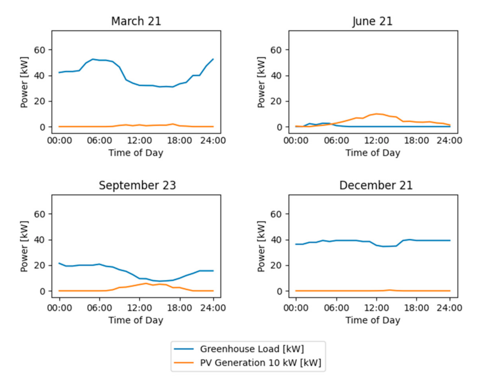
The energy demand of different food and water procurement processes was evaluated. The focus was on the energy demand met by the local microgrid, hence, on the equipment and infrastructure necessary for food and water security, such as greenhouses, water treatment plants, cold storage, and a fish-processing plant. Many other infrastructure modeling options exist, and these were chosen in this scope of analysis due to community preference. Select details on the specific technologies are presented below, with comprehensive information available in Appendix A.

2.1.1. Greenhouse

The energy demand of a community-level greenhouse can be divided into heating and cooling, pumping, and artificial lighting. These factors depend primarily on the amount of available solar irradiance and the ambient temperature. Appendix A.1. presents the relevant equations to model the energy demand of a greenhouse [28,29]. Additional details on modeling plant growth and energy use in the Arctic can be found in the literature [30].

2.1.2. Water Treatment Plant

The energy demand for water treatment plants is composed of lighting, heating, washing, drying, and operation of the central washateria building. This demand has an on-grid component (electrical energy) and an off-grid component, such as heating oil and biomass to produce heat. Since the focus of the analysis was on-grid FEW components, the electrical energy demand of the washateria was modeled with the Alaska Village Electric Load Calculator Tool from NREL [31]. The synthetic hourly data were then calibrated to match the total yearly demand of both a south-central and a southwestern community in Alaska, using monthly electricity usage data provided by the Alaska Native Tribal Health Consortium community reports [32]. The detailed equations and additional information for water treatment plants are presented in Appendix A.2.

2.1.3. Cold Storage

Cooling and freezing loads are a requirement for the produce, fish, and wild game that are an essential part of the lifestyle in remote Alaska communities. The demand associated with cooling and freezing can be divided into four main types of heat loss: transmission, product cooling, infiltration, and miscellaneous load (i.e., people, lights, machinery) [33]. The detailed equations for the cold storage model can be found in Appendix A.3.

2.2. Energy Generation Models

The available power from RE sources was simulated in MATLAB^® Simulink^®. Alaska has experienced a rise in the implementation of renewable power technologies, the most common of which are solar, wind, and hydropower [20]. The following sections describe the modeling for these RE resources. More detail for each model can be found in Appendix B. Modeling according to the following equations requires the input of several values and parameters. In general, the resource time series must be available, including solar radiation, wind speed, river flow rates, and temperature, as well as the desired or already installed nominal capacity. Additionally, each of the following models also requires specific input parameters by the user, as described by the following equations.

2.2.1. Solar PV Model

The solar photovoltaic (PV) model calculates the available power from a solar array. Equation (1) shows the calculation for the DC power output, P_DC [34]:

$${\mathrm{P}}_{\mathrm{DC}}=\frac{\mathrm{G}}{1000\raisebox{1ex}{$\mathrm{W}$}\!\left/ \!\raisebox{-1ex}{${\mathrm{m}}^2$}\right.}{}_{}·{\mathrm{P}}_{\mathrm{STC}}·(1-\mathsf{\beta }\left({\mathrm{T}}_{\mathrm{C}}-{\mathrm{T}}_{\mathrm{STC}}\right)$$

(1)

where ‘G’ is the solar irradiance (kW/m²), ‘P_STC’ is the nominal capacity of the module (kW), ‘β’ is the temperature coefficient of the solar cell (%/°C), ‘T_C’ is the cell temperature (°C), and ‘T_STC’ is the standard test condition temperature (°C). The equations for total irradiance ‘G’ and the cell Temperature ‘T_C’ are further described in Appendix B.1.

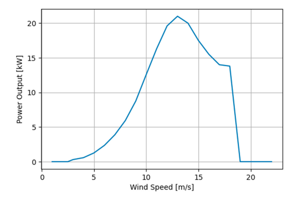
2.2.2. Wind Power Model

The wind turbine generator (WTG) model computes the WTG power output based on the power curve of the turbine, which shows the power output (P_actual) as a function of wind speed at hub height [35]. The maximum theoretically available wind power (P_w) is computed via the kinetic energy, as shown in Equation (2) [35]:

$${\mathrm{P}}_{\mathrm{w}}=0.59·\left(\raisebox{1ex}{$1$}\!\left/ \!\raisebox{-1ex}{$2$}\right.·\mathsf{\rho }·\mathrm{A}·{\mathrm{v}}^3\right)$$

(2)

where ‘ρ’ is the air density (kg/m³), ‘A’ is the swept area of the turbine blades (m²), 0.59 is the Betz limit for wind energy generation efficiency [29], and ‘v’ is the wind speed (m/s) [35]. Additional information and the power curve for the wind turbine are presented in Appendix B.2.

2.2.3. Hydroelectric Power Model

The model for the hydroelectric power plant simulates the available mechanical power, electrical power, and total electrical energy output of small run-of-river hydrokinetic power systems, which are common in Alaska [20]. The mechanical power (P_m) and electrical power (P_e) can be calculated according to Equations (3) and (4) [36]:

$${\mathrm{P}}_{\mathrm{m}}=\mathrm{g}·\mathsf{\delta }·\mathrm{h}·\mathrm{Q}$$

(3)

$${\mathrm{P}}_{\mathrm{e}}={\mathrm{P}}_{\mathrm{m}}·{\mathrm{C}}_{\mathrm{P}}·{\mathsf{\eta }}_{\mathrm{t}}·{\mathsf{\eta }}_{\mathrm{g}}$$

(4)

where ‘g’ is the gravitational constant (m/s²), ‘δ’ is the water density (kg/m³), ‘h’ is the effective head (approximately 80% to 90% of the static head [36]) (m), ‘Q’ is the water flow rate (m³/s), ‘η_t’ is the turbine efficiency (%), and ’η_g’ is the generator efficiency. ‘C_P’ is the power coefficient (%), which represents the ratio of the total hydrokinetic power that can be captured by the turbine blades [36].

2.2.4. Battery Storage Model

The battery energy storage system (BESS) model was adapted from Eteiba et al. [37] and can store excess renewable generation (renewable generation higher than demand) and supply power during times of increased load or low renewable generation. Equations (5) and (6) describe C(t), the available energy content (kWh) in the BESS system during the charging and discharging states [37], respectively:

$${\mathrm{C}}_{\mathrm{charging}}\left(\mathrm{t}\right)=\mathrm{C}\left(\mathrm{t}-1\right)·\left(1-\mathsf{\sigma }\right)+{\mathrm{E}}_{\mathrm{surplus},\mathrm{RE}}·{\mathsf{\eta }}_{\mathrm{BESS},\mathrm{charging}}$$

(5)

$${\mathrm{C}}_{\mathrm{discharging}}\left(\mathrm{t}\right)=\mathrm{C}\left(\mathrm{t}-1\right)·\left(1-\mathsf{\sigma }\right)-{\mathrm{E}}_{\mathrm{deficit}}/{\mathsf{\eta }}_{\mathrm{BESS},\mathrm{discharging}}$$

(6)

where η_{BESS,charging} and η_{BESS,discharging} are the charging and discharging efficiencies, respectively, and ‘σ’ is the self-discharge rate of the BESS. E_surplus,RE and E_deficit are the excess RE generation or the energy deficit (if RE generation is lower than demand), within the limits of the battery’s capacity. The model inputs include the available excess generation (kWh) (charging) or unmet load (discharging), and the model outputs are the state of charge (SOC), additional excess generation, or additional unmet load, which needs to be covered by the diesel-electric generator. The operational SOC in the battery model is between 30% and 90% of the nominal capacity, and the charging and discharging efficiencies are both set to 90%.

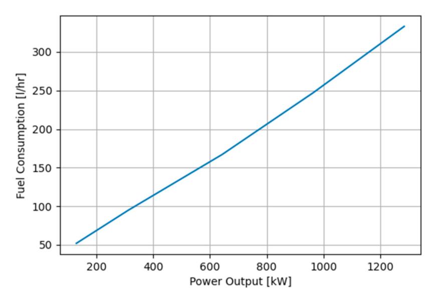
2.2.5. Diesel-Electric Generator Model

The diesel-electric generator is modeled to meet the load that cannot be covered by renewable sources or by the battery system. The diesel-electric generator model has a minimum load equal to 30% of its nominal capacity [38]. Fuel consumption is described by the fuel curve, which must be provided in the model based on existing infrastructure in order to accurately quantify the fuel usage at different operational loading points of the diesel-electric generator. An example fuel curve for a diesel-electric generator is presented in Appendix B.3. The nominal capacity of each diesel-electric generator was sized according to each community’s demand based on available data and represents the existing generator configuration of each community. The implemented dispatch strategy is kept simple, the load that is not covered by renewable generation and battery storage is met by the diesel-electric generators. Due to the relatively high-level modeling scope using a one-hour average resolution, it is assumed that the diesel-electric generators have the necessary ramp rates at finer temporal intervals to deal with load variability caused by RE integration. While significant, more detailed modeling of electric grid frequency regulation and voltage control exceeds the high-level scope of this analysis.

2.3. Energy Distribution Model Parameters and Validation

The energy resource models were created in MATLAB^® Simulink^® and the modeled energy generation was quantitatively validated using HOMER Pro software [27] and the National Renewable Energy Laboratory’s PVWatts tool [39]. The inputs for the validation in HOMER are the same as for the energy resource models in MATLAB^® Simulink^®, including meteorological time series for the renewable resources (e.g., solar radiation) and technology-specific parameters, as specified below.

The solar PV system was designed to be south facing with a tilt of 65°; system losses including those from shading, dirt, snow, and degradation of 15%; an inverter efficiency of 95%; and a temperature coefficient of −0.37%/°C [29]. With irradiance data from a community in interior Alaska [40], the model output exceeded the PVWatts total annual output by less than 2%.

The wind model was analyzed using a power curve adapted from a Windmatic 17S wind turbine [41]. The modeled turbine has a hub height of 25 meters and a blade diameter of 6 meters. The total yearly generation from the model was 5.7% lower compared to the HOMER Pro output. This was most likely due to several reasons, among which are different approaches for air density calculations and slight differences in the power curve.

The hydroelectric plant model in Simulink^® has a 90-meter total head height and 10% head loss [36]. The total annual generation in the model is 2% lower compared to the HOMER Pro output with the same parameters.

3. Results and Discussions from Selected Case Studies

The presented models for RE generation were applied to different case studies in communities throughout Alaska (south-central, south-western, and interior Alaska). It should also be noted that while the communities represent different examples of FEW systems in remote Alaska communities, they do not necessarily represent all community FEW systems in their respective regions. These case studies showed the flexibility and potential of the energy distribution models to inform a community’s decision making on food-energy-water infrastructure.

3.1. Food

The energy demand for food provision includes procurement, processing, and preparation, as well as food storage. In the following subsections, the energy use of some food-related processes and infrastructure was analyzed with regard to the potential implementation and impact of RE.

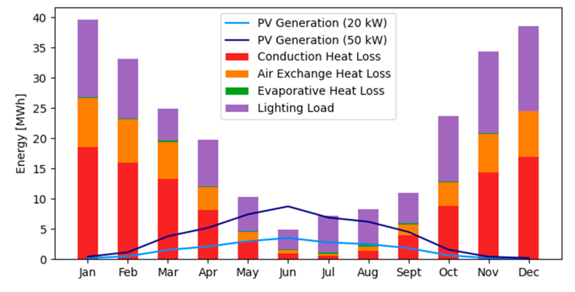
3.1.1. Solar PV for a Greenhouse in Interior Alaska

A community-level greenhouse with an active crop growing area of 167 m² (1800 ft²) was modeled for a community in interior Alaska. Many parameters were required for the modeling of the greenhouse demand, the most important of which were the minimum allowed temperature, which was set to 16 °C (60 °F), and the properties of the construction material [28,29]. These and other parameters can be found in Appendix A.1.

The energy demand of the greenhouse consists of the heating and cooling demand, as well as the artificial lighting required for the crops. The subdivision of the modeled demand is shown in the stacked bars in Figure 2, where the light and dark blue lines represent the monthly generation of a 20-kW and a 50-kW ground-mounted solar PV installation, respectively, highlighting the seasonal mismatch between solar PV generation and the greenhouse energy demand. Since heating represents a large amount of the energy demand throughout the year, the sensitivity of the construction material was observed by changing from double-pane to triple-pane windows. This change was able to reduce the yearly heating demand by 20.2%. There is a strong mismatch between demand and generation due to an assumed year-round operation of the greenhouse; other operational schedules, such as no winter growing, were considered in Section 3.3.2.

In Figure 2, two potential capacities of solar PV were chosen; however, the model can input any size proposed by the community. Remarkably, due to the seasonal mismatch of solar PV generation and the load profile, an increase in installed solar PV or battery capacity will only have a small absolute influence on the amount of the total load covered by renewable generation. For example, a 10-kW solar PV installation with a 100-kW/100-kWh battery system can cover 3.3% of the total load. A 20-kW solar PV array covers 6.5% of the total load and an increase to 50 kW solar PV capacity can meet just below 14% of the total demand. The average annual power demand of the greenhouse is 28.5 kW and 89% of the total energy demand occurs outside of the summer months (June to August); thus, solar output in the summer is not as valuable compared to the winter, when less resource is available. However, with an energy-efficient greenhouse, there is potential for solar power to cover a substantial amount of demand in late spring, summer, and early fall in order to extend the Arctic growing season. To explore this further, Section 3.3.2 presents the energy use for different growing seasons. Additionally, the modeled daily profile of the greenhouse is presented for several days throughout the year in Figure A4 in Appendix D.

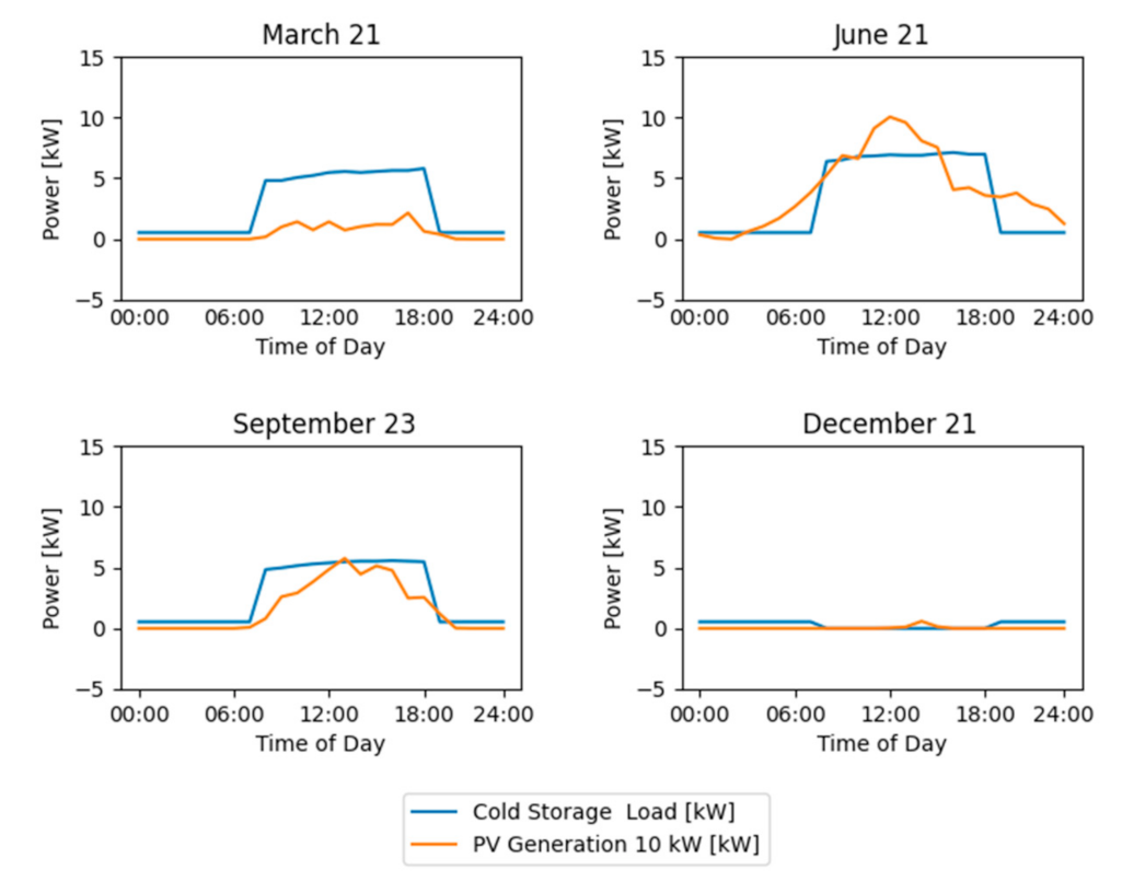
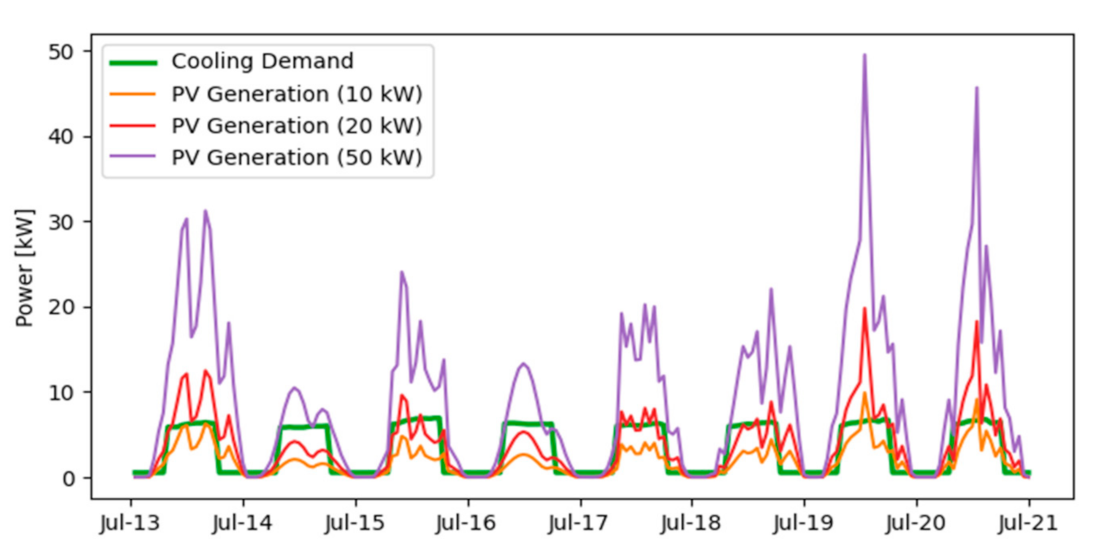
3.1.2. Solar PV for Cold Storage in Interior Alaska

A community-wide cold storage system was explored for a community in interior Alaska, since traditional root cellars are becoming less effective [42] due to a warming climate and ground layer. For the cooling storage model, a 283 m³ (10,000 ft³) building structure with 50% active space usage for cooling product and a cold storage temperature of −5 °C (23 °F) was modeled. A peak cooling load of approximately 7 kW occurs in the summer due to a strong dependence on ambient temperature. The cooling cycle is assumed to have a coefficient of performance (COP) of two, meaning the heat extracted from the cold storage is equal to double the required electric power. Increasing the COP would proportionately increase the heat extraction, with the same electrical input.

With a 5-kW solar PV unit, approximately 42% of the total load (16,300 kWh is the total cooling demand) can be covered, due to an advantageous seasonal overlap of cooling demand and solar PV generation. This can be observed in Figure 3, which shows the hourly load and solar PV generation for several days in the month of July.

Other example calculations with different solar PV capacities of 10 kW, 20 kW, and 50 kW lead to RE penetrations, or the percentage of the load covered by RE, of 61%, 74%, and 81%, respectively. Adding a 100 kW/100 kWh battery energy storage system allows an increase of solar PV penetration to 79%, 89%, and 95% for the three presented solar PV capacities, respectively. During the summer months, the solar PV system is able to cover a substantial amount of the cooling load, as can be observed in Figure 3. This can additionally be observed in Figure A5, which shows the daily profile of the cold storage for select days in different seasons.

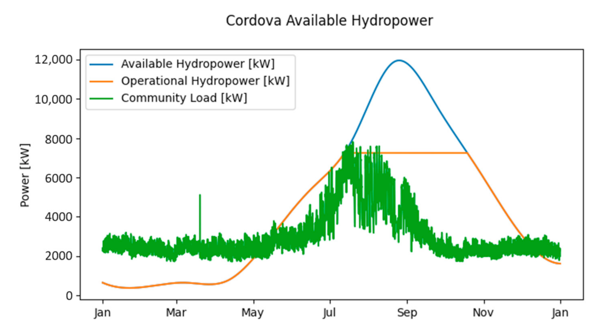
3.1.3. Hydropower for Fish Processing Plant in South-Central Alaska

A community in south-central Alaska is an interesting example of the intricacy of the FEW nexus. A large part of the community’s power demand is covered by two run-of-river hydroelectric plants. The fish-processing plants consume significant amounts of power during the summer months, but also require substantial amounts of water for processing fish, which in turn provide food security (and enhance the local economy). The available hydropower increases significantly from snowmelt in the summer, which coincides well with the additional load of the fish processing plants. This alignment is shown in Figure 4.

The community currently has approximately 7.25 MW of installed hydroelectric capacity, which, according to the ideal model, covers approximately 79% of the community’s yearly load. The electric power demand of the fish-processing plant, which leads to the observed increase in community electric power demand during the summer, can be covered almost exclusively by the hydroelectric power plant. The results were reached by using historical creek flow rates [43,44] applied to Equations (3) and (4) in combination with the community’s load data [45].

The community recently also installed a 1-MW/1-MWh Lithium-ion battery energy storage system, which complements the hydroelectric plant by shifting generation to times of higher demand on a sub-hourly to daily scale, contributing to the higher penetration of RE and reducing reliance on diesel fuel. The battery also provides important reserve capacity and frequency control that improves grid stability.

3.2. Water

The energy demand for water can be subdivided in different stages, such as procurement, treatment, heating, and disposal. For this section, the energy demand for water is focused on the infrastructure for water distribution, also referred to as the washateria. The washateria is typically a centralized building where the community members have access to potable water, showers, washing machines, and dryers.

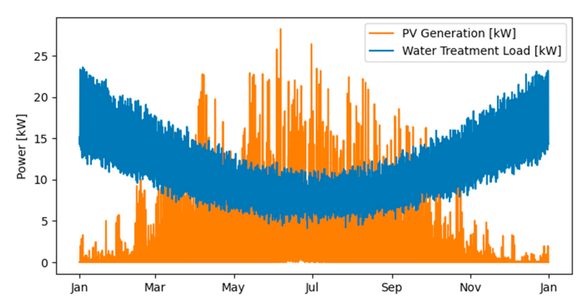
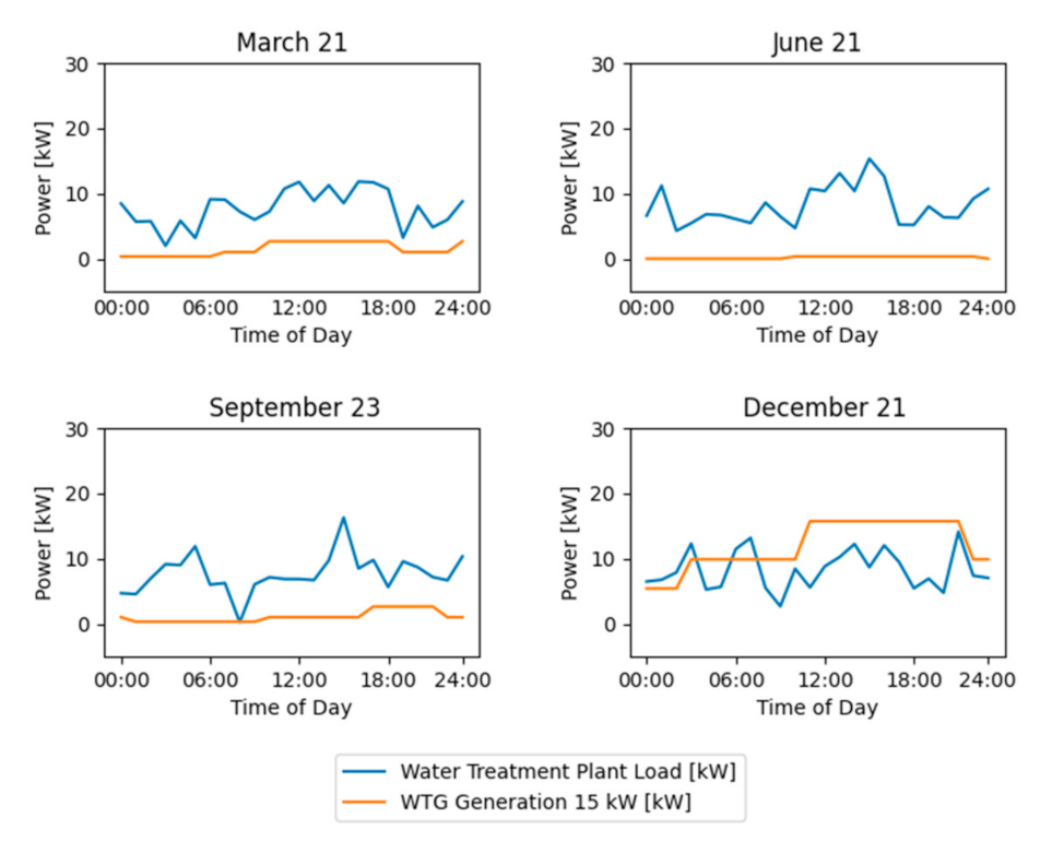
3.2.1. Solar PV for Water Treatment Plant in Interior Alaska

The local washateria in a community in interior Alaska serves as a centralized building for water procurement and washing since there is no piped water distribution system. The washateria energy demand includes lighting, ventilation, and heating, as well as operation of washing machines and dryers [32]. The modeled demand for the water treatment facility is shown in Figure 5, together with the power generated from a 30-kW solar PV installation. The solar PV model, in combination with a 100-kW/100-kWh battery system, is able to cover 28% of the yearly demand.

The water treatment plant demand is at its lowest during summer [46] when solar energy peaks. However, the seasonal variability of the load is not as strong as that of the greenhouse in Section 3.1.1. For the water treatment plant, 19% of the load occurs during the summer months and, overall, the load is spread more evenly throughout the year. This allows solar power to cover a more substantial amount of the load.

Example calculations with 15 kW, 30 kW, and 50 kW solar PV installation capacities show that solar PV can cover 14%, 24%, and 31% of the total yearly load, respectively. These values are respectively more than doubled, compared to the solar PV penetration values of the greenhouse in Section 3.1.1. With the addition of a 100-kW/100-kWh battery energy storage system, the total load coverage of the water treatment plant can be increased to 15%, 28%, and 39%, respectively. For an economic analysis, the increase in penetration must be weighed against the battery storage system costs.

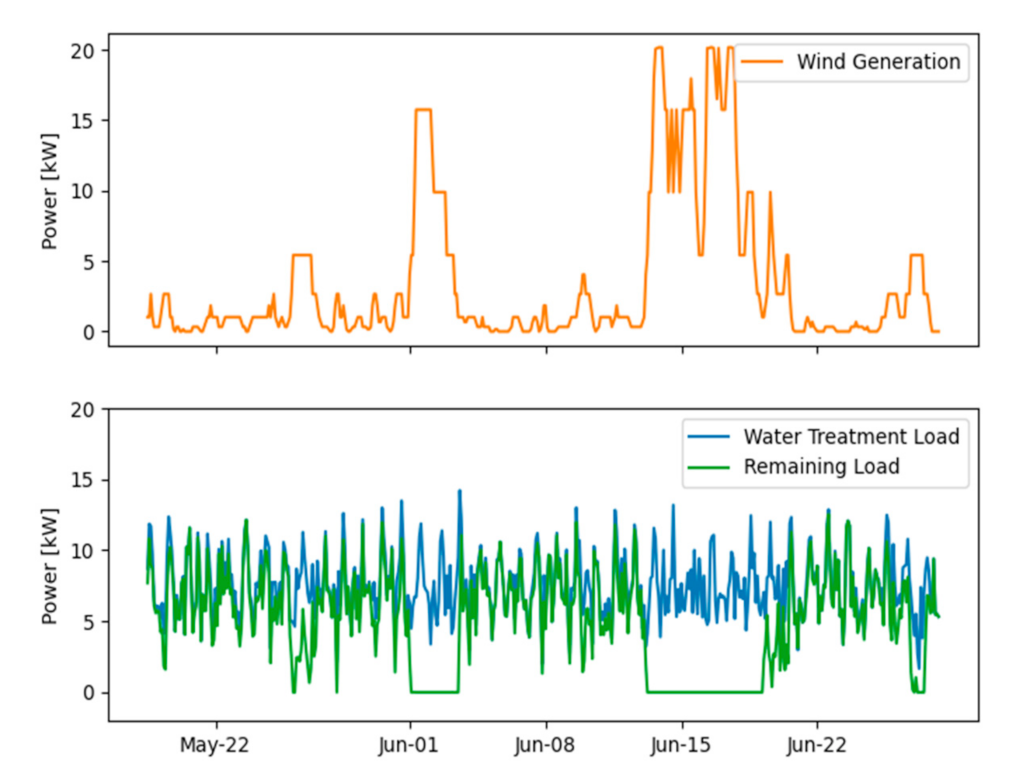
3.2.2. Wind Power for Water Treatment Plant in Southwestern Alaska

The water treatment plant load in a community in southwestern Alaska is similar to the one in the Interior in Section 3.2.1. The demand includes lighting, refrigeration, washers and dryers, as well as space heating and ventilation [32]. Figure 6 shows the wind generation of a 15-kW turbine (top, orange), the total load (bottom, blue), and the remaining load (bottom, green). The remaining load must be met by diesel-electric generators. Wind power does not have the distinct daily and seasonal pattern of solar PV generation. The depicted time frame of one month is representative of the wind power dynamic throughout the entire year, as is also presented in Figure A6, which shows the daily profile of the water treatment plant and wind turbine generator for select days throughout the year. As can be observed in Figure 6, wind power can cover the load of the water treatment plant for several days in a row, followed by multiple days with low generation and consequently, low coverage.

The microgrid of the observed community is a hybrid system with wind turbines and diesel-electric generators. For the water treatment plant, the potential influence of wind turbines is explored in the model. With a 15-kW wind turbine and the wind speed data for this community, the wind power alone is able to cover 43% of the total load, and, in combination with a 100-kW/100-kWh battery energy storage system, the covered load percentage reaches 49%. Increasing the wind turbine nominal capacity to 30 kW improves the RE penetration to 56%, and with a battery, to 65%. A 15-kW turbine with battery energy storage leads to less curtailed power (percentage-wise), as it is a better match for the average washateria load. A 30-kW turbine reaches a higher overall renewable penetration; however, a larger percentage of generated power is curtailed. This can be improved slightly by increasing the battery storage size and can be varied in the model to fit the community’s needs

3.3. FEW Indices

In order to establish a measure for the connection of the different FEW loads, three indices were used. In this research, the FEW nexus was analyzed on a community-scale through an energy lens, which relates the use of energy to food and water procurement: the Energy–Food (EF) and Energy–Water (EW) indices, respectively. Additionally, the Sustainable Energy (SE) index describes the potential RE coverage of the total energy demand of grid-connected FEW loads. The indices were calculated as examples for the FEW components that were presented in the case studies. For a more comprehensive analysis, it is suggested that all the relevant processes of food and water procurement in a community be included. The indices provide a simple and intuitive metric to inform the community on the level of their FEW security and allow for measuring potential improvements within the community, such as integrating RE.

3.3.1. Energy–Water (EW) Index

The Energy–Water (EW) index (based on [5,47]) is a measure for the relation of water and energy use tied to water procurement. Specifically, the EW index is determined by dividing the total water-related energy use by the total water use, as shown in Equation (7):

$$\mathrm{EW}=\frac{{\mathrm{Total}\mathrm{Energy}}_{\mathrm{water}-\mathrm{related}\mathrm{use}}}{\mathrm{Total}\mathrm{Water}}$$

(7)

This index was estimated for two communities, one in interior Alaska and one in southwestern Alaska, encompassing the electricity use of the central washateria building. Some communities may also use off-grid resources, such as wood or heating oil, to cover some of the demand. The total energy use was modeled and calibrated with select collected data, as discussed in Section 3.2. The total water consumption was estimated for each community based on the World Health Organization’s recommendation of 50 liters per person per day [48].

For the community in interior Alaska, the EW index is 21 Wh_el/L (0.021 kWh_el/L) and for the community in southwestern Alaska, it is 9 Wh_el/liter (0.009 kWh_el/L). The substantial difference in the EW index for the observed communities is influenced by several factors. The community in southwestern Alaska, for instance, is located on the coast, with a more moderate climate and more regular solar resource. This leads to an overall lower heating and lighting load, which decreases the EW index since this energy use is associated with water treatment and distribution. Hence, this energy demand is allocated to the EW index, to give the community an understanding of how much energy is being used for water. Additionally, the community in interior Alaska is approximately half the size, in comparison, which may lead to a higher fixed energy demand per person and per quantity of water.

The EW index is not intended for a comparison between communities, as some differences are inherent to the location and other characteristics of the community, as is the case in the above example. The simplicity of the EW index allows the community to quickly estimate the energy use related to water, which can directly be connected to the cost of energy, first in the status quo and then monitor changes in the index after potential RE integration or energy efficiency measures. Consequently, the EW index can be used as a tool to make informed system improvements, such as implementing energy or water efficiency measures, as explored in Section 3.3.4.

3.3.2. Energy-Food (EF) Index

The Energy–Food (EF) index (based on [5,47]) relates the energy use of the food procurement process to the resulting food quantity. The EF index is calculated by dividing the energy required for food production by the resulting total food production, as presented in Equation (8):

$$\mathrm{EF}=\frac{{\mathrm{Total}\mathrm{Energy}}_{\mathrm{food}-\mathrm{related}\mathrm{use}}}{\mathrm{Total}\mathrm{Food}\mathrm{Yield}}$$

(8)

The presented food procurement case studies are a community-level greenhouse and a cold storage building. The EF indices for crop growth in the modeled greenhouse are shown in

Table 1. Crop yield and Energy–Food index for common produce, as calculated with the energy model for a community greenhouse in interior Alaska, considering the assumptions in Appendix A.1. The 4-month period is from May to August, and the 8-month period is from March to October. The cost of energy required per kWh is calculated for each growing period and for each crop in Table A3 in Appendix C.1.

	Energy–Food Index
Crop	4-Month Period (kWh/kg)	8-Month Period (kWh/kg)	12-Month Period (kWh/kg)
Squash	4.6	8.4	13.2
Cucumber	5.1	9.2	14.6
Tomato	10.4	18.8	29.8
Eggplant	13.0	23.5	37.3
Potato	9.9	17.9	28.4
Lettuce	12.4	22.4	35.5
Broccoli	89.2	161.3	255.4

. The results use the assumptions stated in Section 2.1.1, and further in Appendix A.1, including crop yields for small-scale agriculture [49] and the respective duration until harvest (values in

Table A2. Values for estimated growth period for each modeled crop and expected yield in a greenhouse.

Crop	Duration [days]	Source	Yield [kg/m2]	Source
Squash	70	[59]	22	[49]
Cucumber	60	[59]	17	[49]
Tomato	70	[60]	10	[49]
Eggplant	70	[59]	8	[49]
Potato	50	[59]	7	[49]
Lettuce	50	[61]	6	[49]
Broccoli	120	[62]	2	[49]

, Appendix A.1). The values in Table 1 are separated into different growing periods, depending on how long the greenhouse is used throughout the year. The 4-month growing period is the most optimal, as it is conducted during the summer months when artificial heating and lighting demand are the lowest (May to August). The 8-month period (March to October) makes use of the shoulder seasons to increase the total crop yield, whereas the 12-month period assumes a year-round operation.

The values in Table 1 differ substantially among the growth periods and the various crops. The latter is due to the inherent characteristics of the different crops that are factored into the EF index, such as the crop-specific duration until harvest (see Table A2 in Appendix A.1). The differences between the growth periods are due to seasonal changes. The most ideal growth period is limited to the summer months, thus extending the period into the shoulder seasons or into the winter substantially increases the heating and lighting requirements. Beyond this, the resulting EF indices for different crops and different greenhouse operation periods can be used to determine the utility of the greenhouse in comparison to imported produce from an energy use perspective. Since increased or decreased energy use translates to increased or decreased costs, respectively, a simple economic comparison can then be made. This analysis focused on the energy use comparison through the EF indices, rather than the cost and qualitative benefits of locally grown foods.

The greenhouse energy demand is highest when the solar resource is lowest, resulting in substantial differences for solar PV penetration between the different growing periods. For instance, the 4-month growing period (during the summer) requires the least electrical energy while having the highest available solar resources. Consequently, for the most ideal 4-month growing period, the solar PV penetration (SE index in Section 3.3) of a 30-kW solar PV system without a battery energy storage system is approximately 40%. Extending the growing period to 8 months results in 19% solar PV penetration, while a year-round greenhouse operation reaches only 9% solar PV penetration.

The estimation for the cold storage energy use per amount of cooled product, also modeled with meteorological data from interior Alaska, is shown in

Table 2. Cooling demand for community storage unit for different types of food. Meat, fruit, and vegetables can be easily exchanged with similar or other desired products in the model. Values are for a 283-m³ (10,000 ft³) community cold storage in interior Alaska.

	Energy–Food Index (Wh/kg)
Chicken	0.075
Beef	0.075
Fish	0.076
Blueberries	0.094
Broccoli	0.090

.

In order to relate the total yearly energy use of the cold storage unit to the amount of cooling product stored throughout one year, it is assumed the average residence time of a product in the cold storage unit is 3 months. The mentioned product types are considered to be representative for products refrigerated in the observed communities [50]. The differences between food types are comparably small. This is because the thermal properties of the cooled products [33,51,52] are similar, and the product cooling load represents only one component that contributes to the total cooling load.

The tables above show two important components of food procurement in rural Alaska communities, namely greenhouses and cold storage. These results encompass common crops and show the practical application of the proposed methods. Using the EF index as a simple and intuitive metric for the specific energy use of crops in a greenhouse can help the community compare different crops in terms of energy use and inferred cost of energy. The EF indices related to cold storage can help understand the energy use of refrigeration of certain foods. Additionally, these decisions must be considered in the context of availability, accessibility, and quality of the food, as well as the preference and the interests of the community.

3.3.3. Sustainable Energy (SE) Index

The Sustainable Energy (SE) index (based on [5]) is a measure for RE penetration, or the share of the FEW components’ energy demand covered by RE, as described in Equation (9):

$$\mathrm{SE}=\frac{{\mathrm{Renewable}\mathrm{Energy}}_{\mathrm{FEW}\mathrm{Infrastructure}}}{{\mathrm{Total}\mathrm{Energy}\mathrm{Requirement}}_{\mathrm{FEW}\mathrm{Infrastructure}}}$$

(9)

The degree of RE integration depends on temporal, grid stability, and economic factors. Temporal factors include both the daily and seasonal overlap of demand and renewable generation, grid stability factors include the grid’s ability to absorb renewable generation, and economic factors include the capital, installation, maintenance, and operating costs of RE integration.

While solar and wind are studied here due to their relative ease of installation in a remote community, this analysis has shown that they are not always a good direct match for the demand of FEW loads. The results in

Table 3. Sustainable Energy (SE) index on a yearly basis for the computed case studies, tabulated by energy technology. Values for solar PV and wind turbines include a 100-kWh/100-kW battery energy storage system. The SE index shows the renewable penetration for each FEW load, allowing, for example, to see the same solar PV capacity achieves different renewable penetrations for different FEW drivers.

FEW Load (Average Load, Region)	Sustainable Energy Index
	Solar PV Capacity:
	10 kW	30 kW	50 kW
Greenhouse (18 kW, 167 m2, Interior AK)	3%	9%	14%
Cold Storage * (2 kW, 280 m3, Interior AK)	79%	92%	96%
Water Treatment Plant (11 kW, Interior AK)	9%	24%	31%
	Hydrokinetic Capacity:
	5 MW	7 MW	9 MW
Fish Processing Plant and Community (3,070 kW, South-Central AK)	80.0%	80.7%	80.7%
	Wind Turbine Capacity
	5 kW	15 kW	30 kW
Water Treatment Plant (8 kW, Southwestern AK	21%	49%	65%

* Cold storage SE index is higher due to the average load of the cold storage being comparatively low. For the sake of comparison, the solar PV system is chosen to match those of the other FEW components in this table.

summarize the impact of RE in the case studies. The differences between the different FEW loads (e.g., greenhouse and cold storage) demonstrate that the effectiveness of renewable integration depends, to a large degree, on the demand side.

For example, in Table 3 the penetration for a 30-kW solar PV system (and 100-kW/100-kWh battery) achieves a 9% penetration for the year-round operated greenhouse and 24% penetration for the water treatment plant. For cold storage, the SE index is substantially higher because of two main reasons. The average load of the cold storage is smaller compared to the greenhouse and the water treatment plant. and additionally, the seasonal and daily overlap of the cold storage energy demand with solar generation is ideal, as can be observed in Section 3.1.2. This example shows how solar PV can achieve a higher useful penetration when employed for the water treatment plant and cold storage, rather than for the community greenhouse. This simple approach can illustrate the advantages of one RE technology over another, allowing for a more informed decision-making process. It has to be mentioned that in the considered communities the FEW infrastructure can represent a large part of the total load. Additionally, the local utility may not allow for net-metering or any backflow into the main grid, justifying the RE integration being tailored to only specific elements of the grid. This latter aspect must be considered in the context of each community individually.

3.3.4. Indices Application Example

In order to better understand the novelty of the proposed method, an example is hereby presented. A community desires to increase FEW resilience and voices an interest in evaluating growing crops locally in a greenhouse with potential use of RE. With solar radiation data and temperature time series to account for the climate of the community, the research team may suggest a greenhouse size and potential energy efficiency retrofits compared to regular greenhouses. Based on the location, the land availability, and on the weather conditions, the research team evaluates the RE technologies. The results are presented to the community in terms of indices, for several RE types and sizes, in order to provide a simple and intuitive metric for understanding the impact of RE.

Under consideration of the community’s dietary preferences, the results may include the EF index, which provides the energy use of different types of crops (and can be easily translated from kWh/kg into USD/kg based on the cost of energy). Additionally, the community can be presented with suitable RE resources that can be compared using the SE index. In the presented case study, this could mean that solar PV and wind integration was evaluated. Wind power was discarded due to the community not having a good wind resource. The EDM shows an RE integration for solar PV of 3%, 9% and 14% for a solar PV system with 10 kW, 30 kW and 50 kW of nominal capacity, including a 100-kW/100-kWh battery, respectively, for a year-round operation of the greenhouse. An additional analysis shows that with a 30-kW solar PV system and greenhouse operation during the hottest summer months (May to August) or during the shoulder season (March to October), a renewable integration of 40% or 19%, respectively, can be achieved.

This process can be expanded to different FEW loads and can provide the community with tailored suggestions that account for the community’s needs and the available resources.

4. Conclusions and Key Takeaways

This analysis proposed a methodology to model the energy demand of several grid-connected FEW loads, as well as the modeling of commonly used RE sources. The discussed case studies show possible applications of this work by presenting the energy use of FEW loads and observing the influence of RE on those loads.

The adaptation and broader use of this methodology can increase the reliability and security of food, energy, and water (FEW) systems by providing quantitative insights into energy flows of FEW loads in communities. The results of this work illustrate the potential for the implementation of RE in remote Arctic communities to serve FEW loads. However, the findings highlight the need to analyze more diverse technologies to accommodate different types of FEW infrastructure.

The presented energy models based on a bottom-up approach are a useful and adaptable tool that can be applied not only to Arctic and Subarctic communities, but also to remote communities with islanded microgrids in other regions of the world. The Sustainable Energy (SE) index evaluates the penetration of RE for the respective FEW systems, allowing a measure for the effect of RE integration and, thus, for the suitability of different RE technologies. The Energy–Food (EF) and Energy–Water (EW) indices present the energy use for several components of the supply chain for food and water. The indices present the relationship between energy and food and water, providing a measure to assess the advantages and/or shortcomings of FEW systems.

By highlighting and quantifying some of the FEW connections in a simple and intuitive manner, the energy distribution models and their indices provide a tool that can help the communities and utilities make informed community-level decisions and improve FEW security.

Future Work

The case studies selected in this analysis are a limited sample of the applications of the EDM and the indices. Future work may consider a higher diversity of energy technologies, such as heat pumps or biomass reactors. The methods and the resulting insights gained for the Alaska communities are applicable not only to other Arctic and Subarctic communities but also other remote islanded microgrid communities.

The analysis showed the importance of diurnal and seasonal patterns for both the demand and the energy resource. Consequently, demand-side dispatchability can provide additional flexibility to increase the RE penetration, as has been explored to a certain level in previous research work documented in this paper. Modeling in a higher temporal resolution may also provide a higher level of detail for the sizing and penetration of RE technologies. Additionally, considering the renewable penetration for the microgrid as a whole, rather than considering the respective elements separately, can provide deeper insight into the impact of RE on the community and its FEW infrastructure. The results of this work, including the outputs of the EDM models and more directly the FEW indices, are being used to inform a community level FEW security analysis based on four components (availability, access, preference, and quality) that will help remote islanded microgrid communities evaluate and determine the best paths to improve FEW security and reliability.

References

1. McCormick, P.; Awlachew, S.; Abebe, M. Water–Food–Energy–Environment Synergies and Tradeoffs: Major Issues and Case Studies. Water Policy 2008, 10, 23–26. [Google Scholar] [CrossRef]
2. Fan, C.; Lin, Y.; Hu, C. Empirical framework for a relative sustainability evaluation of urbanization on the water–energy–food nexus using simultaneous equation analysis. J. Environ. Res. Public Health 2019, 16, 901. [Google Scholar] [CrossRef] [Green Version]
3. Aboelnga, T.; Khalifa, M.; Mcnamara, I. The Water-Energy-Food Security Nexus: A review of Nexus Literature and Ongoing Initiatives for Policymakers; Nexus Regional Dialogue Programme (NRD): Bonn, Germany, 2018; pp. 25–30. [Google Scholar]
4. Daher, T.; Mohtar, H. Water-energy-food (WEF) Nexus Tool 2.0: Guiding integrative resource planning and decision-making. Water Int. 2015, 40, 748–771. [Google Scholar] [CrossRef]
5. Willis, H.; Groves, D.; Ringel, J. Developing the Pardee RAND Food-Energy-Water Security Index: Toward a Global Standardized, Quantitative, and Transparent Resource Assessment; RAND: Santa Monica, CA, USA, 2016. [Google Scholar]
6. Hussein; Memon, A.; Savic, A. An integrated model to evaluate water-energy-food nexus at a household scale. Environ. Model. Softw. 2016, 93, 366–380. [Google Scholar]
7. Karan, E.; Asadi, S.; Mohtar, R.; Bawaain, M. Towards the optimization of sustainable food-energy-water systems: A stochastic approach. J. Clean. Prod. 2017, 2, 662–674. [Google Scholar] [CrossRef]
8. Horvath, A.; Stokes, J. Water Energy Sustainability Tool (WESTWeb); University of Berkeley: Berkeley, USA, 2020; Available online: https://west.berkeley.edu/model.php#knowledge (accessed on 23 June 2020).
9. Stockholm Environment Institute (SEI). Integrating the WEAP and LEAP Systems to Support Planning and Analysis at the Water-Energy Nexus; SEI: Stockholm, Sweden, 2012. [Google Scholar]
10. D’Odorico, P.; Davis, K.F.; Rosa, L.; Carr, J.A.; Dell’Angelo, D.C.J.; Gephart, J.; MacDonald, G.K.; Seekell, D.A.; Suweis, S.; Rulli, M.C. The Global Food-Energy-Water Nexus. Rev. Geophys. 2018, 56, 456–531. [Google Scholar] [CrossRef]
11. Lofman, D.; Petersen, M.; Bower, A. Water, Energy and Environment Nexus: The California Experience. Int. J. Water Resour. Dev. 2002, 18, 73–85. [Google Scholar] [CrossRef]
12. Siebert; Ruddell, B.L.; Scanlon, R.; Reed, P.M. The food-energy-water nexus: Transforming science for society. Water Resour. Res. Adv. Earth Space Sci. 2017, 53, 3550–3556. [Google Scholar]
13. Schmidt, J.; Johnson, B. Results from the MicroFEW Study (Community Interviews, Food, Energy & Water). 2020. Available online: https://ine.uaf.edu/media/284327/microfewsreport_foodenergywater_august2020-2.pdf (accessed on 8 July 2021).
14. Whitney, E.; Schnabel, W.; Aggarwal, S.; Huang, D.; Wies, R.; Karenzi, J.; Huntington, H.; Schmidt, J.; Dotson, A. MicroFEWs: A food–energy–water systems approach to renewable energy decisions in islanded microgrid communities in rural Alaska. Environ. Eng. Sci. 2019, 36, 7. [Google Scholar] [CrossRef] [PubMed] [Green Version]
15. Hodges, E.; Meter, K. Food in the Last Frontier: Inside Alaska’s Food Security Challenges and Opportunities. Environ. Sci. Policy Sustain. Dev. 2015, 57, 19–23. [Google Scholar]
16. Huntington, H.; Schmidt, J.; Loring, P.; Whitney, E.; Aggarwal, S.; Byrd, A.; Dev, S.; Dotson, A.; Johnson, B.; Karenzi, J.; et al. Applying the food–energy–water nexus concept at the local scale. Nat. Sustain. 2021, 4, 672–679. [Google Scholar] [CrossRef]
17. Demer, L. Power Outages Threaten Subsistence Harvests in Western Alaska Village; Anchorage Daily News: Anchorage, Alaska, USA, 2018. [Google Scholar]
18. Eichelberger, L. Living in Utility Scarcity: Energy and Water Insecurity in Northwest Alaska. Am. J. Public Health 2010, 100, 1010–1018. [Google Scholar] [CrossRef] [PubMed]
19. Mueller-Stoeffels, M.; VanderMeer, J.; Baca, M.; Schenkman, B.; Koplin, C. Cordova Electric Cooperative Energy Storage Evaluation; Sandia National Laboratories: Albuquerque, NM, USA, 2017.
20. Renewable Energy Alaska Project (REAP); Renewable Energy Atlas of Alaska: Anchorage, AK, USA, 2020.
21. Holdmann, G.; Wies, R.; Vandermeer, J. Renewable Energy Integration in Alaska’s Remote Islanded Microgrids: Economic Drivers, Technical Strategies, Technological Niche, and Policy Implications. Proc. IEEE 2019, 7, 1820–1837. [Google Scholar] [CrossRef]
22. Alaska Energy Authority. Power Cost Equalization Program Statistical Report; FY: 2012–2020. Available online: http://www.akenergyauthority.org/What-We-Do/Power-Cost-Equalization/PCE-Reports-Publications (accessed on 17 April 2021).
23. Wies, R. (Electrical and Computer Engineering Department, College of Engineering and Mines, University of Alaska Fairbanks, Fairbanks, AK, USA). Personal Communication, 2020.
24. White, D.; Schubert, D.; Woolard, C. Water Supply and Waste Treatment in the Arctic. Available online: https://education.uarctic.org/media/334571/BCS312_mod6.pdf (accessed on 17 April 2021).
25. Meter, K.; Goldenberg, M. Building Food Security in Alaska; Alaska Department of Health and Social Services, with Collaboration from the Alaska Policy Council: Minneapolis, MN, USA, 2014. [Google Scholar]
26. Loring, P.; Gerlach, S.; Harrison, H. Seafood as local food: Food security and locally caught seafood on Alaska’s Kenai Peninsula. J. Agric. 2013, 3, 13–41. [Google Scholar] [CrossRef] [Green Version]
27. Homer Energy by UL. Homer Pro. Available online: https://www.homerenergy.com/products/pro/index.html (accessed on 14 April 2021).
28. Aldrich, A.; Bartok, W. Greenhouse Engineering; Natural Resource Agriculture and Engineering Services (NRAES): Ithaca, NY, USA, 1994. [Google Scholar]
29. Masters, G. Renewable and Efficient Electric Power Systems; Wiley Interscience: Hoboken, NJ, USA, 2004. [Google Scholar]
30. Sambor, D.; Wilber, M.; Whitney, E.; Jacobson, M.Z. Development of a tool for optimizing solar and battery storage for container farming in a remote arctic microgrid. Energies 2020, 13, 5143. [Google Scholar] [CrossRef]
31. Devine, M.; Baring-Gould, E. The Alaska Village Electric Load Calculator; NREL: Denver, CO, USA, 2004. [Google Scholar]
32. ANTHC, Alaska Native Tribal Health Consortium. Rural Energy Reports & Community Audits. Available online: https://anthc.org/what-we-do/rural-energy/audits/ (accessed on 14 April 2020).
33. Ghajar, J.; Cengels, A. Refrigeration and Freezing of Foods. Heat Mass Transf, 5th ed.; McGraw Hill Education: New York, NY, USA, 2015. [Google Scholar]
34. Hellman, P.; Lehtonen, M.; Koivisto, M. Photovoltaic Power Generation Hourly Modeling. In Proceedings of the 2014 15th international scientific conference on Electric Power Engineering (EPE), Brno-Bystrc, Czech Republic, 12–14 May 2014; pp. 269–272. [Google Scholar] [CrossRef]
35. Agrawal, A.; Wies, R.; Johnson, R. Hybrid Electric Power Systems: Modeling, Optimization and Control; VDM Verlag Dr. Mueller: Riga, Latvia, 2014. [Google Scholar]
36. El-Sharkawi, A. An Introduction to Electric Energy; CRC: Boca Raton, FL, USA, 2012. [Google Scholar]
37. Eteiba, M.; Barakat, S.; Samy, M.; Wahba, I. Optimization of an off-grid PV and Biomass hybrid system with different battery technologies. Sustain. Cities Soc. 2018, 40, 713–727. [Google Scholar] [CrossRef]
38. Vandermeer, J.; Light, D.; Alaska Center for Energy and Power (ACEP), University of Alaska Fairbanks, Fairbanks, AK, USA. Personal Communication, 2020.
39. National Renewable Energy Laboratory. PVWatts Calculator; NREL. Available online: https://pvwatts.nrel.gov/ (accessed on 7 April 2021).
40. National Renewable Energy Laboratory. National Solar Radiation Data Base (Data for Fairbanks, AK). Available online: https://rredc.nrel.gov/solar/old_data/nsrdb/ (accessed on 11 February 2020).
41. Windmatic, A.S. Windmatic 17S Data Sheet. Available online: http://windmatic.com/WM17S-Brochure.pdf (accessed on 23 April 2021).
42. Schmidt, J.; Johnson, B. Food, Energy and Water: Results from the MicroFEW Study (Renewable Energy). 2020. Available online: https://ine.uaf.edu/media/284326/microfewscommunityreport_re_july62020.pdf (accessed on 17 May 2021).
43. Alaska Department of Natural Resources. Division of Mining, Land, and Water, The State of Alaska. Available online: http://dnr.alaska.gov/mlw/water/hydro/streams/streams.cfm (accessed on 20 March 2021).
44. Summit Construction Consultants. Final Technical and Construction Report for Power Creek Hydroelectric Project in Cordova, Alaska; Cordova Electric Cooperative, Inc.: Cordova, AK, USA, 2002. [Google Scholar]
45. Alaska Energy Data Gateway. Operational Powerhouse Data. 2011. Available online: https://psi.alaska.edu/data/ (accessed on 1 February 2020).
46. Rashedin, M.; Subhabrata, D.; Whitney, E.; Madden, D.; Aggarwal, S. Energy consumption for domestic water treatment and distribution in remote Alaska communities. In Proceedings of the Research Poster AGU Fall Meeting, Online Conference, 7 October 2020. [Google Scholar]
47. Jones & Wagener, The WEF Nexus Index. Available online: https://wefnexusindex.org/ (accessed on 15 June 2021).
48. World Health Organization. Media Brief; The Human Right to Water and Sanitation. Available online: https://www.un.org/waterforlifedecade/pdf/human_right_to_water_and_sanitation_media_brief.pdf (accessed on 12 February 2021).
49. Rabin, J.; Zinati, G. Yield Expectations for Mixed Stand, Small-Scale Agriculture. Sustain. Farming Urban Fringe 2012, 7, 1–4. [Google Scholar]
50. Arctic Health. Final Report on the Alaska Traditional Diet Survey, 2004. Available online: arctichealth.org (accessed on 23 April 2021).
51. The Engineering Toolbox. Specific Heat of Food and Foodstuff. Available online: https://www.engineeringtoolbox.com/specific-heat-capacity-food-d_295.html (accessed on 5 April 2021).
52. ASHRAE. Thermals Properties of Food; R09 SI: Atlanta, GA, USA, 2006. [Google Scholar]
53. Torres, P.; Lopez, G. Commercial Greenhouse Production: Measuring Daily Light Integral in a Greenhouse; Purdue Extension, Purdue Department of Horticulture and Landscape Architecture: Lafayette, IN, USA, 2010. [Google Scholar]
54. Sager, J.; Farlane, C.M. Radiation, Chapter 1. Available online: https://www.controlledenvironments.org/wp-content/uploads/sites/6/2017/06/Ch01.pdf (accessed on 22 June 2021).
55. Mattson, N. Greenhouse Lighting; Cornell University: Ithaca, NY, USA.
56. Frouin, R.; Pinker, R. Estimating Photosynthetically Active Radiation (PAR) at the earth’s surface from satellite observations. Elsevier Remote Sens. Environ. 1995, 51, 98–107. [Google Scholar] [CrossRef]
57. Greenhouse Management. Does Light Transmission through Greenhouse Glazing Matter? Available online: https://www.greenhousemag.com/article/does-light-transmission-through-greenhouse-glazing-matter/ (accessed on 18 May 2021).
58. Randolph, J.; Masters, G. Energy for Sustainability, 2nd ed.; Foundations for Technology, Planning, and Policy, Island Press: Washington, DC, USA, 2008. [Google Scholar]
59. Albert, S.; Vegetable Harvest Times. Harvest to Table. Available online: https://harvesttotable.com/vegetable_harvest_times/#:~:text=Early%20varieties%20will%20be%20ready,second%20harvest%20from%20early%20varieties (accessed on 11 May 2021).
60. McGee, K. How Many Days From Seeds to Tomato Plants? June 2020. Available online: https://homeguides.sfgate.com/many-days-seeds-tomato-plants-56852.html (accessed on 12 May 2021).
61. Burpee, “All About Lettuce,” Burpee. Available online: https://www.burpee.com/gardenadvicecenter/vegetables/lettuce/all-about-lettuce/article10236.html#:~:text=Most%20lettuce%20varieties%20mature%20in,crisphead%2070%20to%20100%20days. (accessed on 11 May 2021).
62. Albert, S. How to Grow Broccoli, Harvest to Table. Available online: https://harvesttotable.com/how_to_grow_broccoli/#:~:text=Broccoli%20grown%20from%20seed%20will,are%20still%20green%20and%20tight (accessed on 12 May 2021).
63. Seifert, R. Special Considerations for Building in Alaska. University of Alaska, Fairbanks; Cooperative Extension Service: Fairbanks, AK, USA, August 2000.
64. Ugwu, H.; Ogbonnaya, E. Design and Adaptation of a Commercial Cold Storage Room for Umudike Community and Environs. IOSR J. Eng. 2012, 2, 1234–1250. [Google Scholar]
65. CAT. Diesel Generator Sets 3516 B. Available online: https://www.cat.com/en_US/products/new/power-systems/electric-power/diesel-generator-sets/18331799.html (accessed on 12 May 2021).
66. Alaska Energy Authority. Power Cost Equalization Program Statistical Report; FY: 2020. Available online: http://www.akenergyauthority.org/Portals/0/About/Board%20Meetings/Documents/2020/FY20%20PCE%20Statistical%20Report%20-%20Community%20Version.pdf (accessed on 15 June 2021).
Figure 1. Examples of on-grid and off-grid loads and drivers of FEW security in remote Alaska.
Sustainability 13 09511 g001
Figure 2. Composition of greenhouse monthly energy demand shown in contrast to the solar PV monthly generation. The yearly profile of the greenhouse is inverse to the solar generation, because heating is a substantial energy requirement and is thus highest in the winter when the solar resource is lowest.
Sustainability 13 09511 g002
Figure 3. Hourly cooling load of cold storage in interior Alaska and renewable solar PV generation, which can be used for a cooling cycle during a selected summer week representative of varying amounts of solar resource.
Sustainability 13 09511 g003
Figure 4. Available hydropower at hydroelectric plant and installed capacity in comparison with the community load. The load can be covered almost entirely by the installed hydroelectric plant during summer and autumn months.
Sustainability 13 09511 g004
Figure 5. Modeled water treatment plant demand in interior Alaska and solar PV generation of a 30-kW solar PV system. The solar PV generation is able to cover a large amount of the load from spring until early autumn.
Sustainability 13 09511 g005
Figure 6. Wind turbine generation for 15 kW nominal capacity, total water treatment plant load, and load not met by renewable sources covered by diesel-electric generation. The wind generation in combination with a battery storage system can cover the entire load for several days in a row.
Sustainability 13 09511 g006