Article

Study on the Sharing Transportation Based on Game Theory

School of Modern Post, Beijing University of Posts and Telecommunications, Beijing 100876, China
*
Author to whom correspondence should be addressed.
Sustainability 2021, 13(16), 9347; https://doi.org/10.3390/su13169347
Submission received: 15 June 2021 / Revised: 6 August 2021 / Accepted: 13 August 2021 / Published: 20 August 2021
(This article belongs to the Topic Industrial Engineering and Management)

Abstract

:
In order to solve the problems of mismatch between transportation resources and order volume in logistics transportation, we propose a cooperative pattern called sharing transportation to solve this problems. In this pattern, several logistics enterprises or alliances cooperate with each other and share transportation resources to achieve the goal of reducing costs and increasing income. In this paper, we set the application scene of sharing transportation to the section from the distribution center to the service outlets in the city. We first put forward the judgment function in the analysis model of cooperative pattern, and the possible cooperative pattern is divided into three kinds by constructing and solving the replication dynamic equation. Then we proposed the income allocation model by considering the functions of order quantity and overall income. Moreover, the proposed models are extended to the multi-agent game situation to realize the sharing transportation of multiple enterprises. Finally, we use the example simulation and sensitivity analysis to verify the rationality of the model. This paper provides a new idea for how to integrate the surplus resources to increase the profit in the process of logistics transportation.

1. Introduction

1.1. Background

The sharing economy (SE) is a popular economic model at present, it involves sectors such as transportation, accommodation, entertainment and technology [1]. Sharing logistics(SL) is a new branch of the sharing economy. Compared with the homestay form of lodging, car sharing, bike sharing and charge bank sharing have been put into the market, but sharing logistics still exist on a small scale or even in the stage of theoretical research. Take China as an example. In March 2020, the Sharing Economy Research Center of the State Information Center released The Report on the Development of China’s Sharing Economy [2], which pointed out a lot of shocking data related to the SE in 2019. The market turnover of China’s SE was CNY 3282.8 billion, an increase of 11.6% over the previous year. Employment in the SE has maintained rapid growth, with 6.23 million employees on the platform, an increase of 4.2% over the previous year. SE has played a more significant role in improving the structure of the service sector and promoting the transformation of consumption patterns. In addition, enterprises with sharing economy models in transportation, catering and accommodation accounted for 37.1%, 12.4% and 7.3% of the industry, respectively, which are 20.5, 7.8 and 3.8 percentage points higher than 2016. Meanwhile, the popularizing rate of online car-hailing, take-out meals, shared accommodation and shared medical care up 15.1%, 21.58%, 4.7% and 7% over 2016. We can see that SE has a very large market in China, but the shared logistics does not have much application in the market. However, based on the prosperity and development of SE today, the broad prospects of SL can be anticipated.
In addition, with the further expansion and development of e-commerce in recent years, the logistics industry has received extensive attention. In 2018, Gross Merchandise Volume (GMV) achieves USD 29.16 trillion with year-on-year growth of 11.7% in China [3]. It is obvious that the rise of e-commerce has also brought the logistics industry into a golden period of high order volume, high turnover and high-speed development. In this context, the optimization of the operation cost and operation efficiency of logistics has become an urgent problem. There is no doubt that SL is one of the important development directions of Sharing Economy.
The content of this paper focuses on the transportation part of SL, including the cooperative pattern between logistics enterprises and the income allocation after the cooperation. We propose the idea of adopting the pattern of cooperation between logistics enterprises or alliances in the transportation section from the distribution center in the city to the service outlet in each district. In many cases, the order quantity and transportation capacity of different logistics enterprises and alliances do not match. For example, some logistics enterprises with strong financial resources have strong transportation capacity, but they will face problems such as high empty load rate of trucks and excess transportation capacity. At the same time, some enterprises obtain a large number of logistics orders by means of cooperation with merchants and e-commerce platforms, but they do not have enough transportation capacity, which is prone to problems such as decreased transportation quality and loss of orders. In addition, at present, many logistics enterprises form regional alliances (such as Cainiao Alliance) through mutual shareholding. Such logistics alliances will also join the cooperation system of SL due to the overall uncoordinated excess capacity or excess orders and other problems. Among the problems studied in this paper, there are some issues to be considered, such as whether enterprises or alliances cooperate, cooperative pattern and income allocation pattern under reasonable cooperative pattern. The key to the problem lies in how to establish a reasonable and win-win income allocation mechanism between the two logistics systems. The paper focuses on the problem of cooperative pattern and income allocation of the sharing logistics.

1.2. Literature Review

Sharing logistics (SL) is an important branch of the sharing economy. In previous studies, scholars have done a lot of discussion and analysis on sharing logistics and sharing economy, respectively. In addition, game theory is also an important research method applied in various fields in recent years. As a result, we use the method of game theory to solve the problem.

1.2.1. Related Work of Sharing Economy

The sharing economy (SE) is still a relatively new concept today. As a result, there is no consensus on the definition of the sharing economy. Literature provides several definitions of the SE. Some authors define the SE as the sharing of unique and underutilized resources through commercial and non-commercial means based on the Internet platform without the transfer of ownership [4,5,6]. Clauss et al. argued the SE as the models based on the platform which allow the change from an ownership society to a sharing one [7]. Belk define the SE as the acquisition and allocation of resources through commercial and non-commercial compensation [8].

1.2.2. Research on Sharing Logistics

In order to optimize the allocation of logistics resources, reduce the waste of logistics resources, reduce logistics costs and improve logistics benefits, Wang [9] proposed the concept of sharing logistics. Many studies have pointed out that sharing logistics is beneficial to enhance the interests of cooperation entities. Qin et al. [10] proposed that the advantages of shared service strategies continue to increase with the increase of logistics service levels and market potential. When the logistics service level or market potential increases to a certain level, it will lead to a win–win situation. He et al. [11] proposed that if the price is within a certain range, two companies can improve Pareto through logistics service sharing (LSS). When the price of shared logistics services is below a threshold, the social welfare with LSS will be greater than the social welfare without LSS. In addition, sharing logistics has been applied in many real scenes, which has strong practical significance and reference value. Stephanus [12] studied the application of sharing logistics of resource interoperability in Singapore. Wang et al. [13] took Chongqing as an example to prove the effectiveness of the collaborative mechanism and optimization algorithm of sharing logistics. In addition, Marcucci et al. [14] took Rome’s limited traffic zone as an example, and combined the discrete choice model with the agent-based model, considering the heterogeneous preferences and interaction effects of stakeholders, which better supported the real participatory decision-making process of freight related policies, through building consensus and minimizing the efficiency loss caused by the negotiation process.
In order to improve the benefits of the various entities in the entire logistics supply chain, scholars have done extensive research on different research objects. He et al. [15] studied the impacts of logistics resource sharing on B2C E-commerce companies and customers. Li et al. [16] did evolutionary game analysis of cooperation between high-speed express and express enterprises. In addition, due to the different types of shared resources, the research methods and results are also quite different. Luo et al. [17] studied sharing logistics service supply chain with revenue-sharing and cost-sharing contracts. Taking Velox (a global logistics organization) as an example, Wong and Davision [18] studied the impact and contribution of knowledge sharing in theory, practice and methods. Taking Vietnam’s logistics industry as an example, in view of its market scale and cost factors, Pham et al. [19] studied supply chain partners, sharing methods and influencing factors of the sharing practice between information logistics enterprises and their supply chain partners.
With the development of sharing logistics at home and abroad, through sharing resources to achieve a reasonable distribution of orders among cooperative enterprises has gradually become an important means to reduce costs and increase efficiency in the main and end links of logistics field, especially suitable for the special transportation field which is affected by national special policies and systems and has high technical requirements. Stephanus [12] studied sharing logistics of resource interoperability for the last mile against Singapore’s restrictions on the vehicle types. Wang et al. [13] studied the optimal profit distribution plan that benefits from long-term cooperation in the field of cold chain logistics by restricting the minimum cost and total cost of special vehicles (refrigerated vehicles).

1.2.3. Application of Game Theory

Game theory is known for its research achievements in the economic field, but in recent years it has been widely used in various fields of research. Khojasteh [20] use game theory and the robust optimization to obtain a robust energy procurement strategy for the Micro-grid Operator in smart allocation grids with hydrogen-based energy resources. They proposed an energy procurement strategy of MGO to balance the price of electricity with the electricity demand of customers. Chen [21] utilize cooperative game-theory approaches (the Cournot game and the Shapley value) to find the benefit allocation balance in the cooperation of automation transformation in Hong Kong warehousing industry. Zhang et al. [22] selected evolutionary game model to investigate the optimal selection of two modes (outsourcing mode and authorization mode) in the cooperation of two leading original equipment manufacturers and two third-party remanufacturers in remanufacturing industry. Bukvi et al. [23] used the congestion game for route selection, so as to well analyze the routing problems of competitive logistics operators on the transport network consisting of three Eastern Adriatic ports and an intermodal terminal in Budapest. Based on the comparison of different methods of game theory, Tatarczak [24] analyzed the methods of profit distribution among members of the fourth party logistics supply chain alliance system.

1.3. Contribution of This Paper

The paper models the actual scene of sharing transportation to analyze the cooperative pattern and income allocation under three patterns of cooperation, combining evolutionary games and dynamic games innovatively. The main contributions can be summarized as follows:
(1) The complex scene of sharing transportation is parameterized by means of evolutionary game. In the evolutionary game stage, we carefully considered the various factors affecting the choice of cooperation or not. These influencing factors are integrated and adjusted into some reasonable parameters. Through these parameters, the paper described the game process of the cooperation pattern concisely and accurately. Then the judgment function is given by copy dynamic equation. This judgment function has extraordinary guiding significance to reality. Enterprises can calculate whether they should cooperate or not by calculating the judgment function.
(2) This paper simplifies the game scene through the characteristics of the infinite round game model. In the study of profit distribution, we simplify the game scene through the characteristics of the infinite round game model. Since the actual scene of sharing transportation is very complicated, it is impossible to draw conclusions by considering too many parameters. This paper applies the theory of infinite round games to greatly reduce the number of parameters, but at the same time retain the accuracy of the conclusion. In the conclusion, the optimal distribution pattern and the income of enterprises are calculated.
(3) This paper extends the scene to that of multi-agent game. In sharing transportation, there often exist more than two game agents. To our best knowledge, the existing literature simply divides the multi-agent game into a two-agent game, or focuses on a certain game, such as using the Nash core to solve the n-person cooperative in a dynamic game. In this paper, we divide multi-agent games into three sub-situations: one-to-one, one-to-many, and many-to-many. Through these three situations, various complicated situations in multi-agent games are considered.

1.4. Overview of Each Section of This Paper

Section 1, respectively, introduces the background, literature reviews, contributions, and finally introduces the overview of each section of the paper. Section 2 mainly describes the research scene and gives a brief introduction to our proposed solutions. Section 3 formulates two main model to determine the cooperation pattern of both sides of the game, and solve the maximum income and optimal income distribution. Section 4 analyzes the model and draws valuable conclusions. Section 5 studies the cooperation pattern of multi-agent game. Section 6 sets up the parameters in line with the actual situation to carry out simulation verification and does sensitivity analysis. Section 7 gives a summary of this paper.

2. Problem Statement

The problem scene studied in this paper is that logistics enterprises lacking capacity and providing capacity share resources to reduce costs and increase efficiency, thereby promoting the healthy and rapid development of the entire supply chain. In order to show the problem to be stated in this study clearly, we have drawn the following illustration.
As shown by the red dashed box in Figure 1, the carrying capacity of logistics enterprises or alliances often cannot match the number of orders obtained in the actual logistics transportation scene.
On the one hand, due to the influence of festivals and large-scale promotional activities, the number of logistics orders will increase by hundreds to thousands of times in a short period of time. In order to resist this huge pressure, many large logistics enterprises choose to invest a lot of money to purchase vehicles, equipment and hire labor, which, however, is superfluous for daily transportation work. Furthermore, if the logistics enterprises whose infrastructure has just started choose to explore newer markets, the number of logistics orders is insufficient.
On the other hand, the logistics enterprises that cooperate and reach agreements with merchants and websites, usually have much more logistics orders. However, limited by capital, personnel, etc., they may not have enough transport capacity to match these orders. As shown by the black dashed box in Figure 1, such enterprises are usually named logistics enterprises lacking capacity.
Therefore, the logistics enterprises lacking capacity can share the resources of enterprises providing capacity to avoid the loss of orders caused by the lack of transport capacity, and achieve a win–win effect by reasonable distribution of interests.
In this paper, considering that there are three transport modes of land, air and sea in long-distance transportation across provinces and cities, it is not easy to coordinate systematically so that we define the cooperative transport section as the part of the distribution center to service outlet of one city. At the same time, we simulate the real negotiation scene, in which the smaller enterprises (alliances) should take the lead in bidding, then the two sides play a game to produce the final income allocation and pricing.
Based on the above practical applications and practical scene, a model is formulated to study the cooperative pattern and income allocation of transportation part of SL.

3. Model Formulation

In the formulation of the cooperative pattern model, we mainly solve the cooperative pattern between cooperative enterprise A and B by studying the expected profit conditions. According to the evolutionary game, we define that the two enterprises have the following three cooperative patterns in the transportation segment studied:
  • Pattern 1: Enterprise B shares its own resources to help A to transport.
  • Pattern 2: Enterprise A shares its own resources to help B to transport.
  • Pattern 3: Enterprise A and Enterprise B share resources with each other to help transport.
Sharing resources mentioned above means sharing vehicle resources, human resources, information resources, etc.
In order to analyze the optimal income allocation in three patterns, we firstly formulate the overall income model to solve the optimal overall income function, and we formulate the bargaining game model to solve the optimal income allocation pattern in the cooperation process.

3.1. Cooperative Pattern Analysis

3.1.1. Preliminaries

I: Notations
Before formulating the model, we calibrate the research object, research goal and some of the parameters involved to complete the preparatory work. The following parameters are determined from cooperative pattern analysis and income allocation analysis. The notations related to the cooperative pattern analysis are summarized in Table 1.
First of all, the object of model research is two game subjects with cooperative and competitive relationship, enterprise A and B. Two game players each have two strategic choices, cooperation or non-cooperation. Cooperation is recorded as Y, non-cooperation is recorded as N.
Secondly, calibrate the probability of enterprise A to cooperate as x; then, calibrate the probability of enterprise B to cooperate as y, where 0 ≤ x ≤ 1, 0 ≤ y ≤ 1. The larger the value of x, the greater the tendency of enterprise A to choose cooperation. Similarly, the larger the value of y, the greater the tendency of enterprise B to choose cooperation. Discuss two extreme cases: when x, y = 0, the two parties do not cooperate at all and when x, y = 1, the two parties adopt full cooperation approach. Li [16] used a similar parameter assumption method in the analysis of cooperation between high-speed rail express and express delivery enterprises. The research extended and expanded it on the basis of it.
Besides, since both enterprise A and B have their own original business, we assume the overall profit of operating their own business is π 1 , π 2 , where π 1 , π 2 ≥ 0; when enterprise A and B conduct two-way cooperation, the overall profit of both parties is calibrated as π 1 , π 2 ; when enterprise A unilaterally shares resources with B, the overall profit of both parties is calibrated as π 3 , π 4 ; when enterprise B unilaterally shares resources with A, the overall profit of both parties is calibrated as π 5 , π 6 ; and when enterprise A and B have cooperation negotiations but the cooperation fails, due to the upfront cost, the overall profit of both parties still changes, demarcated as π 7 , π 8 .
II: Necessary assumptions
Assumption 1: Assuming that due to the cooperation of enterprise A and B, one party needs to pay a certain risk cost to the other party when helping the other party in delivering while it also needs to bear the risk cost incurred when the other party delivers its own express delivery. We sum the two risk costs and get the total risk cost of one party’s enterprise, record the total risk cost of enterprise A and B as b, b .
Assumption 2: Regardless of whether the cooperation between enterprise A and B is successful in the end, it is assumed that in order to promote mutual cooperation, both parties will consume a certain amount of negotiation cost. The proportion coefficient of negotiation cost shared by both parties under different cooperation states is shown in Table 2.
Assumption 3: After enterprise A and B cooperate and share resources, their respective benefits will also change accordingly. Suppose that the amount of change in the logistics enterprise’s profit after cooperation is only affected by the following parts: the profit of helping the cooperative logistics enterprise to deliver express delivery, the payment of the cost of helping the cooperative logistics enterprise to deliver express delivery, risk cost expenditure and negotiation cost.
Assumption 4: In different cooperative patterns, it is assumed that market environment is the same, which includes the total amount of orders available for competition in the market, the user’s perception coefficient of transport speed, the user’s perception coefficient of freight and other conditions determined by the market are fixed and do not change with the change of cooperative pattern.
III: Overall cooperation profit function
As the two enterprises cooperate and share resources, the utilization of corporate resources and the efficiency of transportation have changed. As a result, the total revenue of the logistics enterprise has also changed significantly. Based on Assumption 2, Assumption 3, and Assumption 4, this paper will concretely calculate the profit function of enterprise A and B after cooperation, to prepare for the construction of the final model. There are two parts in the profit function. The first part is the increase in corporate profits after cooperation, and the latter part is the basic profits of the enterprise.
The parameter setting table can be shown as Table 3.
For enterprise A, the profit after cooperation is calculated out:
π = s 1 · m 1 + p 1 · n 1 + s 1 · n 2 p 2 · n 2 b n c · c
For enterprise B, the profit after cooperation is calculated out:
π = s 2 · m 2 + p 2 · n 2 + s 2 · n 1 p 1 · n 1 b ( 1 n c ) · c

3.1.2. Model Formulation

According to the parameters assumed in the previous section and the formulation of the evolutionary game model, the profit eagle dove table is as follows (Table 4):
According to the profit matrix in the eagle dove table, when enterprise A chooses to share resources, enterprise B may share or not. When two-way sharing, the profit of cooperative enterprise A is π 1 ; when only enterprise A shares resources with B, the profit of A is π 3 . The expected profit when the cooperative enterprise A chooses to share resources is:
E h c = y · π 1 + ( 1 y ) · π 3
Similarly, when the cooperative enterprise A chooses not to share resources, the expected profit is:
E h n = y · π 5 + ( 1 y ) · π 7
Then the average profit of cooperative enterprise A is:
E h = x E h c + ( 1 x ) E h n = x [ y π 1 + ( 1 y ) π 3 ] + ( 1 x ) [ y π 5 + ( 1 y ) π 7 ]
From the above equations of E h c and E h , the dynamic equation for copying when cooperative enterprise A shares resources is:
F ( x ) = d x d t = x ( E h c E h ) = x ( 1 x ) ( E h c E h h ) = x ( 1 x ) [ y ( π 1 π 5 ) + ( 1 y ) ( π 3 π 7 ) ]
Similarly, the dynamic equation for copying when cooperative enterprise B shares resources is:
F ( y ) = d y d t = x ( E h c E h ) = y ( 1 y ) ( E h c E h h ) = y ( 1 y ) [ x ( π 2 π 4 ) + ( 1 x ) ( π 6 π 8 ) ]

3.2. Income Allocation Analysis

In this paper, the overall revenue model is formulated to solve the most reasonable market pricing and to obtain the optimal overall income. Then the bargaining game model is formulated to solve the respective benefits of each cooperative enterprise (the profit allocation method of SL).
We have supplemented the following assumptions for the two models formulated above to be better unified:
In Pattern 1, enterprise A is the one with the larger volume. A seeks out enterprise B with the lowest price on the market by means of open bidding in the market, the chamber of commerce, etc. Furthermore, B can fully bear the demand of sharing transportation of A in the discussed transportation section. Furthermore, in Pattern 2, A is the one with the larger volume. A seeks out cooperative enterprise B with the lowest price on the market by means of open bidding in the market, the chamber of commerce, etc. Furthermore, A can fully bear the demand of sharing transportation of B in the discussed transportation section. In Pattern 3, two enterprises cooperate become a logistics alliance in the form of mutual investment through reasonable negotiation.
I: Overall income model
The overall income model parameter setting table can be shown as Table 5.
According to the actual situation and relevant research, we can easily know that: when other factors are the same and the transportation speed is faster, users will be more willing to choose the logistics service, and when other factors are equal and the freight is lower, users will be more likely to choose the logistics service. At the same time, the order volume available to the logistics enterprise is the order volume that can be competed for in the market minus the non-ideal loss of the order volume due to speed and freight. The overall income brought by logistics transportation in this transportation section can be defined as the multiplication of the order volume and the price. Therefore, the following function model is formulated:
Order quantity function:
Q = a k 1 t k 2 p
Overall income function:
W = Q · p = ( a k 1 t k 2 p ) · p
II: Bargaining game model
The bargaining game model parameter setting table can be shown as Table 6.
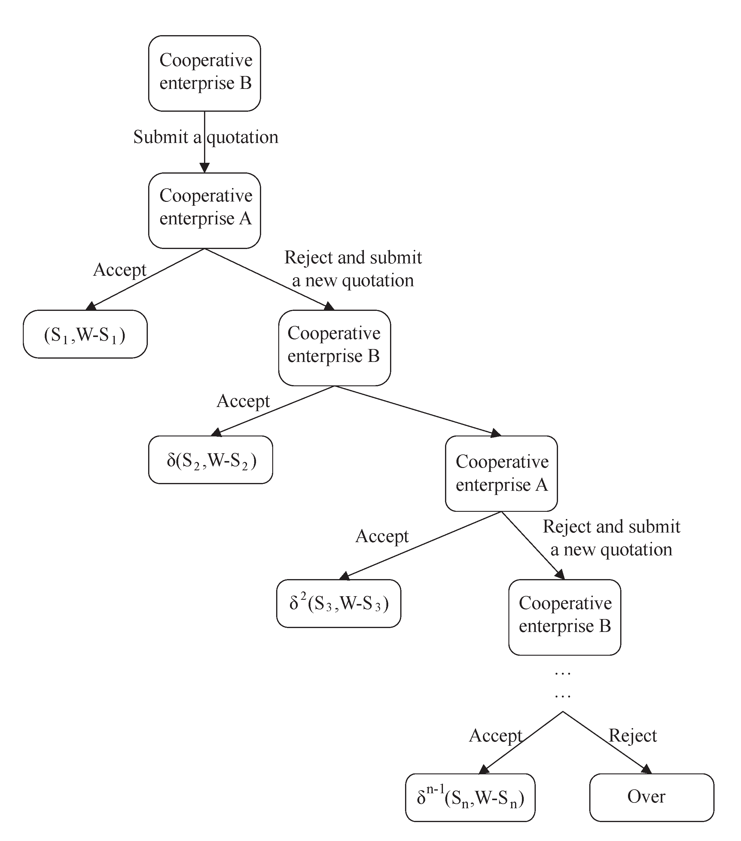
An infinite round bargaining game model is formulated here to simulate the real negotiation scene. It is assumed that at the nth round in the negotiation process, the proposed income allocation method is (S n , W − S n ), the income allocation of cooperative enterprise A is S n , the income allocation of cooperative enterprise B is W − S n , then the negotiation scene of income allocation can be summarized as Figure 2.
A previous paper takes two independent enterprises as the research subject and studies the bargaining game and income allocation between them. This study guides the direction for enterprises to better realize the income maximization in the whole transportation. However, in the actual competition and cooperation scene, there is often a strong combination of several enterprises. The cooperative enterprises can realize the sharing of resources or part of resources, reduce business costs, gather competitive strength, to achieve the goal of maximizing the self-income of the enterprise.
Therefore, based on the “game between two logistics enterprises” model, this part will expand the study of the “game between logistics enterprises and enterprise alliances” model and the “game between two logistics enterprise alliances” model. Hereby, a set of enterprises that are associated with each other is defined as an "enterprise alliance" for the convenience of reference below.

4. Analysis

4.1. Cooperative Pattern Analysis

(1) Analysis of equilibrium point of evolution process
According to the method proposed by Friedman [25], the stability of the equilibrium point of the game system can be derived from the local stability of the Jacobian matrix of the system. Let Formulas (4) and (5) equal to 0, the system equilibrium point can be obtained: O (0,0), A (0,1), B (1,0), C (1,1), and D (p, q).
p = π 8 π 6 π 2 π 4 π 6 + π 8
q = π 7 π 3 π 1 π 5 π 3 + π 7
(2) Local stability analysis of equilibrium point
Finding the partial derivatives of F(x) and F(y) with respect to x and y, respectively, the determinant and trace of the Jacobian matrix J can be obtained:
D e t ( J ) =         ( 1 2 x ) [ y ( π 1 π 5 ) + ( 1 y ) ( π 3 π 7 ) ] x ( 1 x ) ( π 1 π 5 π 3 + π 7 ) y ( 1 y ) ( π 2 π 4 π 6 + π 8 ) ( 1 2 y ) [ x ( π 2 π 4 ) + ( 1 x ) ( π 6 π 8 ]
t r ( J ) = ( 1 2 x ) [ y ( π 1 π 5 ) + ( 1 y ) ( π 3 π 7 ) ] + ( 1 2 y ) [ x ( π 2 π 4 ) + ( 1 x ) ( π 6 π 8 ) ]
Analyze the local stability of the system, 16 cases are shown in Table 7, Table 8, Table 9, Table 10, Table 11 and Table 12. Table 7 describes local stability analysis results in case 1 to case 3; Table 8 describes local stability analysis results in case 4 to case 6; Table 9 describes local stability analysis results in case 7 to case 9; Table 10 describes local stability analysis results in case 10 to case 12; Table 11 describes local stability analysis results in case 13 to case 15; and Table 12 describes local stability analysis results in case 16.
(3) Analysis of evolution results
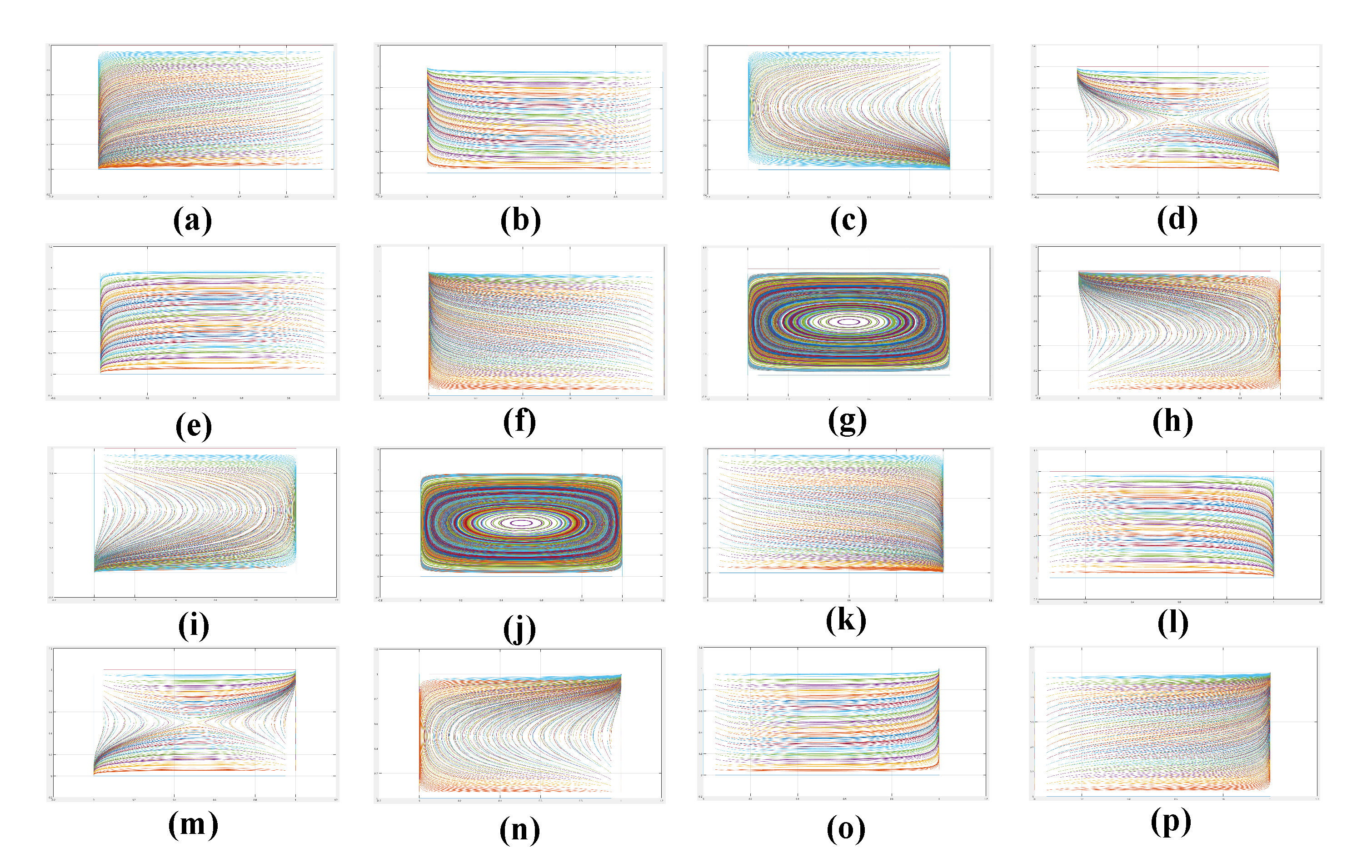
According to the above calculation and analysis, it can be concluded that there are 16 kinds of evolutionary equalization results of the system. The copy dynamic phase diagram is shown in Figure 3.
Conclusion:
  • As shown in Figure 3a,e,i, regardless of the initial state of the system, the two parties cannot achieve a win–win cooperation in the end. The system will tend to an evolutionary stable point (0,0). The two parties will adopt a non-cooperative strategy.
  • As shown in Figure 3b,f,h, (0,1) is the stable point of the evolution of the game between the two parties: enterprise A does not help enterprise B to transport express, while enterprise B helps enterprise A to transport express.
  • As shown in Figure 3c,d,k,l, (1,0) is the stable point of the evolution of the game between the two parties: enterprise B does not help A to transport express, while A helps B to transport express.
  • As shown in Figure 3m,n,o,p, (1,1) is the stable point of the evolution of the game between the two sides: both enterprises help each other to transport express.
  • As shown in Figure 3g,j, the system has no stable point.
Through the above analysis, under different income conditions, the final result of the game between the two parties mainly evolves into three situations: non-cooperation, cooperation, and one-way cooperation. To date, the research has obtained the actual situation corresponding to the sixteen evolutionary results. Realize the parameterization of the real scene, and get the specific recommendation strategy according to the enterprise situation. The model of the thesis allows enterprises to get the most favorable choice in various situations.

4.2. Income Allocation Analysis

In this part, through the formulation of the order quantity function and overall income function, we solve the maximum income and allocation patterns of enterprises under the situation of one-way sharing resources and both sides sharing resources.
According to the Equations (8) and (9), we can solve and then get, when
p = a k 1 t 2 k 2
The maximum value of the overall income function can be obtained:
W ( max ) = ( a k 1 t ) 2 4 k 2
Thereafter, the study analyzes the income allocation model according to the three alternative cooperative patterns above:
I: Pattern 1
Based on the research of Shaked and Sutton on infinite round game in Economic Game Theory [26]:
Step1: According to the study of “three-round bargaining game model”, the optimal solution of the model is as follows:
Player 1 puts forward its own benefit W 1 = W − W · δ + δ 2 S in the first round; Player 2 accepts and gets W 2 = W · δ δ 2 . Since the application scene of "three-round bargaining game model" is inconsistent with the scene discussed in this paper. The research further promotes the infinite bargaining game as follows.
Step2: It is assumed that the infinite round bargaining game has an inverse inductive solution, in which the benefits of A and B are S and W − S, respectively. Namely, A proposes its own benefit S in the first round while B accepts it. According to the infinite round game model, the bargaining starts from the third round in the same scene as the bargaining starts from the first round, that is, A proposes its own benefit S in the third round, B accepts it. In the circumstance, the benefits of both parties are S and W − S, respectively.
S = W W · δ + δ 2 S
To deduce
S = W 1 + δ
Step3: In this infinite round bargaining game, the result of equilibrium optimal solution is as follows: cooperative enterprise A bids in the first round:
S = W 1 + δ
B receives and obtains benefit:
W S = W · δ 1 + δ
Put the above research results into the income allocation model constructed above:
According to the Equation (15) and optimal solution allocation of the above infinite round game model, the maximum income allocation of the two enterprises is:
A:
W 1 ( max ) = ( a k 1 t ) 2 4 k 2 ( 1 + δ )
B:
W 2 ( max ) = δ ( a k 1 t ) 2 4 k 2 ( 1 + δ )
II: Pattern 2
Similarly, when A completely helps B, assuming that B makes an offer first and A puts forward the allocation plan first in the negotiation process, the maximum income allocation of the two enterprises is:
A:
W 1 ( max ) = δ ( a k 1 t ) 2 4 k 2 ( 1 + δ )
B:
W 2 ( max ) = ( a k 1 t ) 2 4 k 2 ( 1 + δ )
III: Pattern 3
If Pattern 3 turned out to be the best cooperative pattern through modeling and analysis, then A and B should formulate a logistics alliance (similar to the Cainiao Logistics) through reasonable negotiation, completely share resources, transport all orders together. Moreover, they should carry out the income allocation refer to the stake, the resources invest and so on. The logistics alliance’s overall income is:
W ( max ) = W ( max )

5. Model Extension

In the previous part, we discussed the cooperation between the two enterprises. However, in reality, multiple enterprises will participate in the preliminary cooperation negotiation process. In order to take this situation into account, we extend the model to a multi-agent situation.

5.1. Additional Assumptions

To simplify the problem research, the extended model weakens the bargaining game among subjects and ignores the differences in competitiveness of different subjects within each alliance. Therefore, different subjects within the same alliance have the same business parameters, such as freight, quantity, operating and administrative expenses, negotiation costs and so on. Moreover, each subject within the same enterprise alliance has the same cooperative strategy.

5.2. Model Analysis

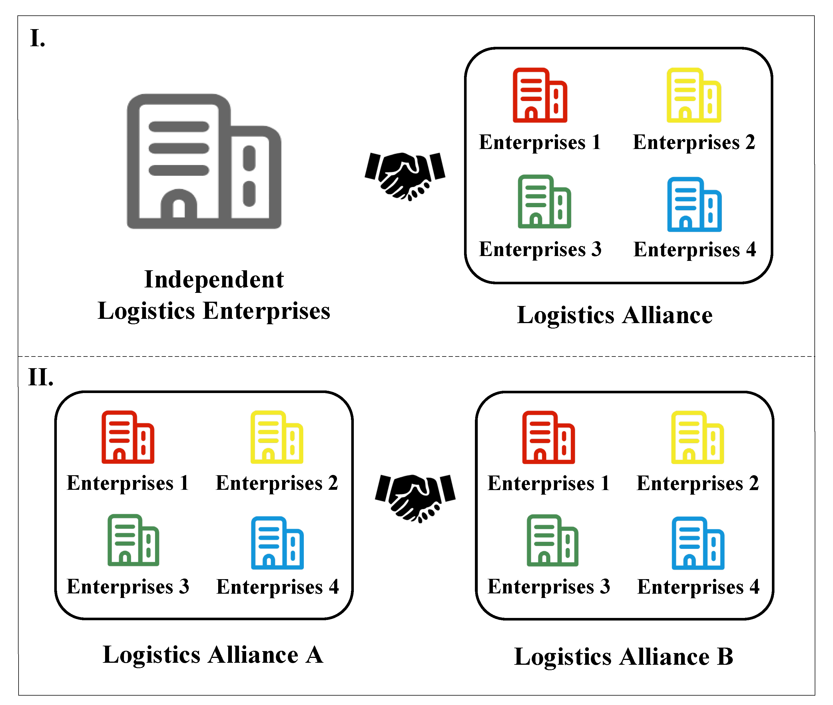
In the case of cooperation between multiple enterprises, the enterprises will first negotiate in pairs, and some enterprises will form alliances. Therefore, the entire negotiation situation of multi-enterprise cooperation only includes the following three situations: one enterprise and one enterprise, one enterprise and one logistics alliance, and two logistics alliances.
Since the logistics alliance is a consortium of two or more enterprises, and its nature is basically similar to that of a logistics enterprise, we can regard the above three negotiation situations as a dual-agent game. Based on this, we extended the model to multi-enterprise cooperation, as shown in the following Figure 4.
On the one hand, based on all the above assumptions, the profit before and after the enterprise alliance participates in the game is expressed with known parameters, and then the eagle-pigeon table of the game between the two parties is constructed. Furthermore, according to the profit after sharing resources, the copy dynamic equation and the Jacobian matrix of the system is solved, and then the stable point coordinates is solved. Finally, by analyzing all the combinations of different parameter value conditions, the stability of this situation is figured out.
On the other hand, the enterprise transportation income function is designed according to the actual logistics and transportation situation. Moreover, the maximum income model is constructed and the maximum income is solved, the bargaining game model is constructed and the best income distribution mode in each case is solved.

5.3. Meaning of the Model Extension

In the logistics industry, multiple enterprises cooperate with each other, to realize resource sharing and formulate a logistics transportation system is bound to become the future trend. This part of the study simplifies it, restricts the constraint conditions, extends the cooperation between two logistics enterprises model, improves the value of theoretical research and model application.
At the same time, in the actual scene, many logistics enterprises have used alliances to seize the market (such as holding shares of each other, etc.). Therefore, extending the model to a number of express delivery enterprises is a very meaningful extension of the market.

6. Example Simulation

In this part, we mainly simulate the model. First of all, we set the simulation data on the public platform and combining with actual survey results, which involves the preset of express freight, etc. Secondly, we analyze the change of income of both enterprises affected by cooperation and sharing. Then, the paper studies the allocation of enterprise income after the game, and verifies the rationality of the preset express freight. Finally, the sensitivity analysis of freight, income distribution mode and the maximum income is studied.

6.1. Parameter Assignment

By querying relevant data released on the public platform of Express Query Tool [27] and combining with actual survey results, we assign values to each parameter in the model built above, as shown in Table 13 and Table 14.

6.2. Simulation Analysis

6.2.1. Analysis of Willingness to Cooperate

Based on the data in Table 13, it can be calculated out: π 1 π 5 > 0, π 2 π 4 > 0, π 3 π 7 > 0, π 6 π 8 > 0, which corresponds to Conclusion Section 4 in the previous part of the paper. In other words, both enterprises tend to help each other to transport express.

6.2.2. Analysis of Profit Growth

In order to see the impact of cooperative transportation on the enterprise more intuitively, we calculated the profit changes before and after the cooperation between enterprise A and enterprise B.
For enterprise A, the change profit of A after cooperation is calculated out:
Δ π = p 1 n 1 + S 1 n 2 p 2 n 2 b 1 n c 1 c = 489
For enterprise B, the change profit of B after cooperation is calculated out:
Δ π = p 2 n 2 + S 2 n 1 p 1 n 1 b 2 ( 1 n c 1 ) c = 189
Therefore, under the cooperative pattern which enterprise A and enterprise B both help each other in transportation, the profits of both parties will increase.

6.2.3. Income Allocation and Preset Freight Verification

Since the analysis of income and cost is often carried out in two parts separately, in this part, we mainly study the income distribution of the subjects participating in the game. At the same time, we verify the pricing of transporting the express preset in the previous part of the paper.
According to the Equation (15) and the assign values shown in Table 14, W ( max ) is calculated.
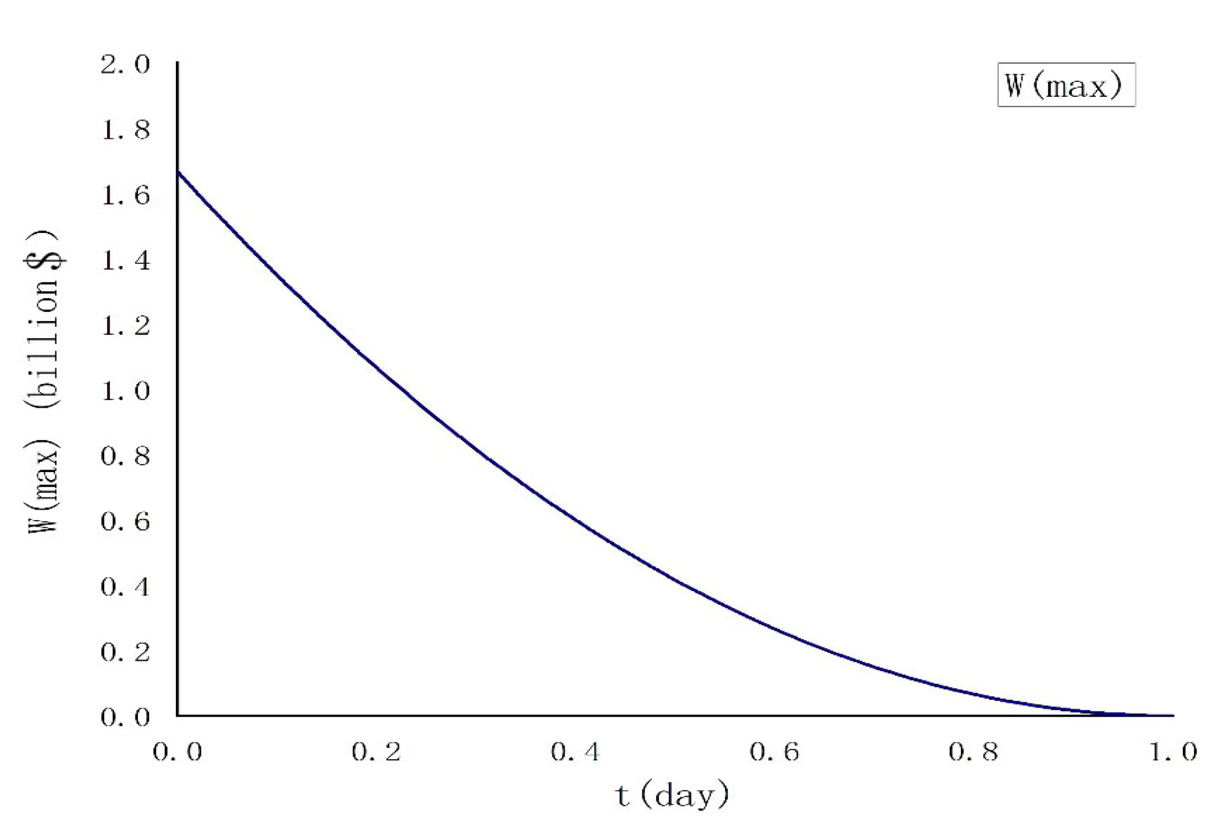
W ( max ) = ( 1 t ) 2 0.6
As the average transportation time increases, the average freight and overall income are shown in the following Table 15.
According to the data of p in the table above, the preset freight is reasonable. The W(max)-t relational figure is Figure 5:
Next, we will discuss the income distribution of both sides of the game under the three patterns, and study the dynamic relationship between market competitiveness and freight of transporting express.
I: Pattern 1
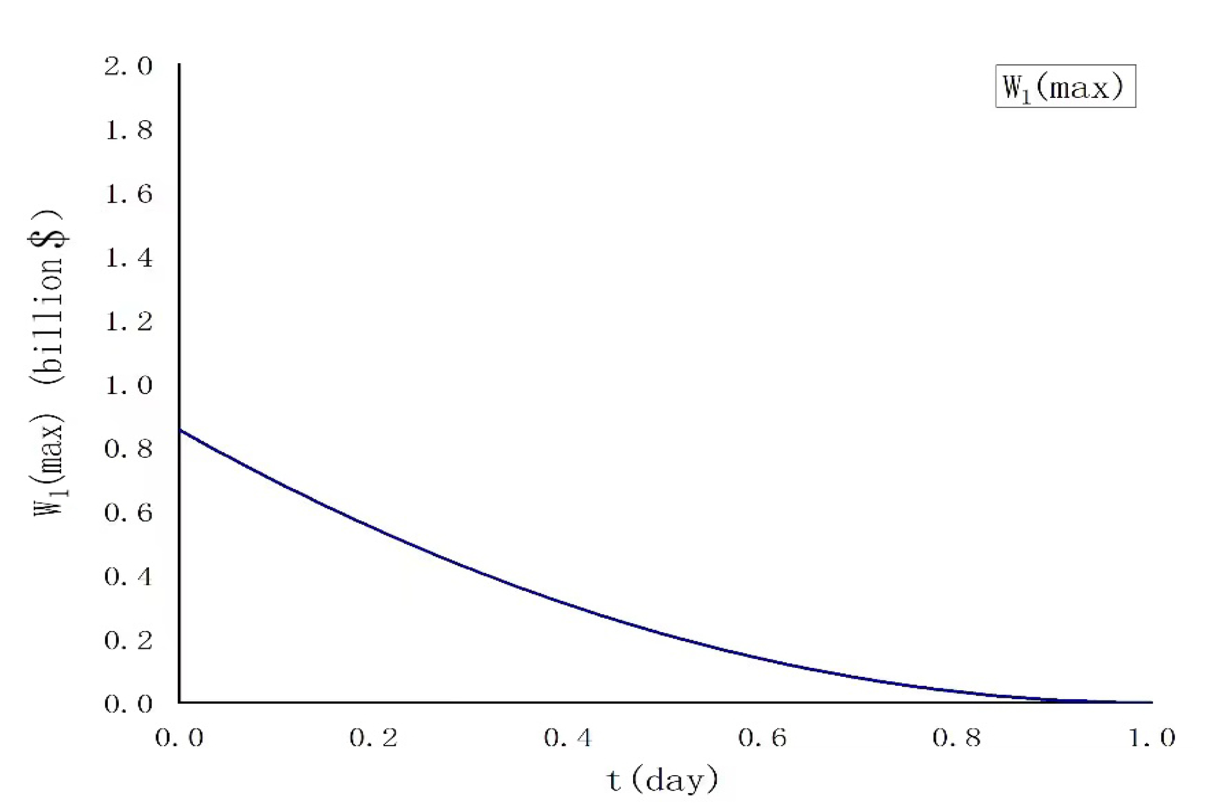
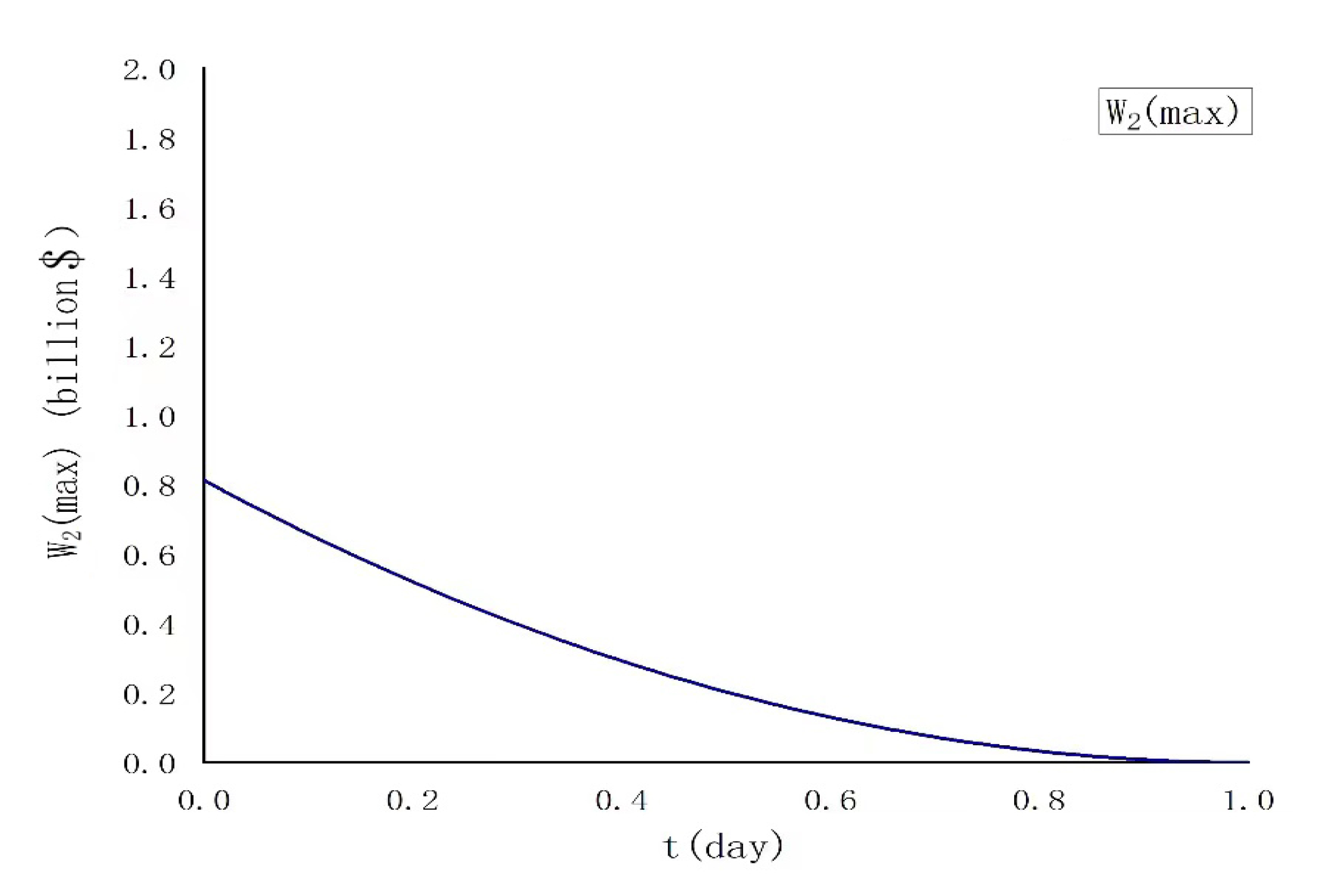
According to the Equation (20), (21) and the assign values shown in Table 14, W 1 ( max ) and W 2 ( max ) is calculated.
W 1 ( max ) = ( 1 t ) 2 1.17
W 2 ( max ) = ( 1 t ) 2 1.23
In the case of A unilaterally helping B transport, the income allocated to enterprise A is calculated, as shown in Table 16.
The W 1 (max)-t relational figure is Figure 6:
In the case of A unilaterally helping B transport, the income allocated to enterprise B is calculated, as shown in Table 17.
The W 2 (max)-t relational figure is Figure 7:
Pattern 2
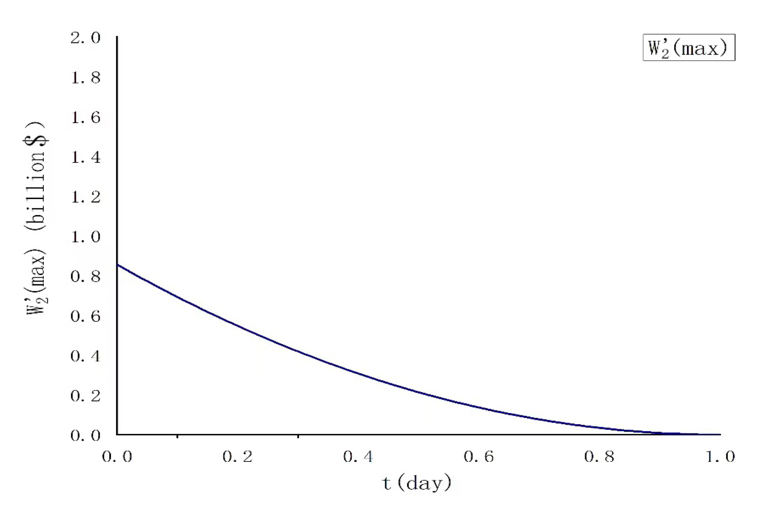
According to the Equation (22), (23) and the assign values shown in Table 14, W 1 ( max ) and W 2 ( max ) is calculated.
W 1 ( max ) = ( 1 t ) 2 1.23
W 2 ( max ) = ( 1 t ) 2 1.17
In the case of enterprise B unilaterally helping A transport, the income allocated to enterprise A is calculated, as shown in Table 18.
The relational figure is Figure 8:
In the case of enterprise B unilaterally helping A transport, the income allocated to enterprise B is calculated, as shown in Table 19.
The W 2 (max)-t relational figure is Figure 9:
III: Pattern 3
According to the Equation (24) and the assign values shown in Table 14, W ( max ) is calculated.
W ( max ) = ( 1 t ) 2 0.6
Then under different transportation times, the maximum value of income of the alliance are shown in the following Table 20.
The W (max)-t relational figure is Figure 10:
In the previous part, we can see that the solution results of the models in the three patterns are all within a reasonable range and in line with our expectations after introducing the assumed parameters. Considering the actual transportation time and pricing strategy, we only focus on the function change of t between 0 and 2 days. We can see that in the three patterns, the overall income and the income of A and B (such as W 1 , W 2 ) all reach the maximum value when t is infinitely approaching 0; equal to 0 when t is equal to 1; and negative when t is greater than 0.
Meanwhile, with the increase of t, income decreases gradually. This functional feature is in line with the reality: in logistics transportation, the shorter transportation time will gain more customers’ favor and more income. However, in the logistics transportation in cities, one day’s transportation time is obviously long and the competitiveness is poor. Therefore, in this model, when t = 1, the enterprise will have zero income because it cannot get orders, and even suffer a loss when t > 1.

6.3. Sensitivity Analysis

In the part, we conduct sensitivity analysis on the model, find out several parameters in the model that have great influence on the cooperation income, analyze the reasons and the important factors that play a leading role, improve the reliability and flexibility of cooperation evaluation. We conducted sensitivity analysis from the following three aspects, as shown below.

6.3.1. Sensitivity Analysis of Factors Affecting Freight

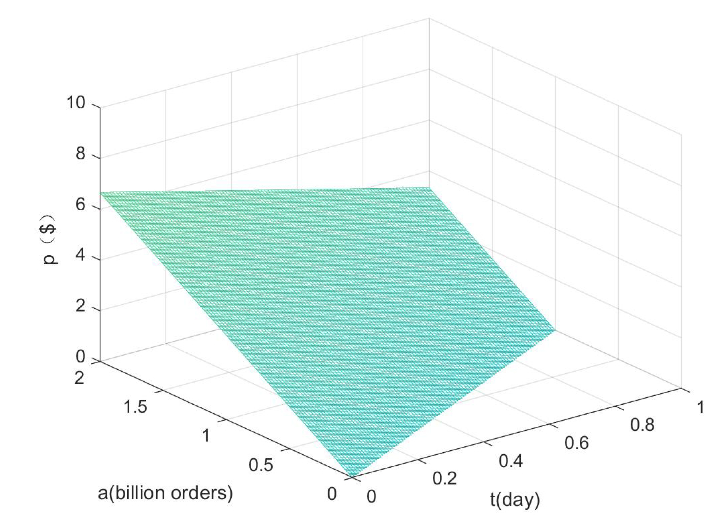
It can be seen that the change of the values of a and t will affect the optimal value of freight, where p and a are directly proportional with a proportional coefficient of 3.33. p and t are directly proportional with a proportional coefficient of −3.33. The influence of a and t on p is shown in Figure 11. In the actual application scene, the market a is around billion orders, t is about 0.6 days, p is about USD 1.5. Therefore, the base value of a in this sensitivity analysis is billion orders, the base value of a is 0.6 days.
We can get the rate of change of p-a relational table as Table 21:
We can get the rate of change of p-a relational table as Table 22:
As can be seen from the above tables and images, a and t have the same influence on the value of freight p while the influence is great. a changes by 20% near the base value, making the freight p change by about 50%. t changes by 33% near the base value, making the freight p change by about 50%.

6.3.2. Sensitivity Analysis of Factors Affecting the Maximum Income

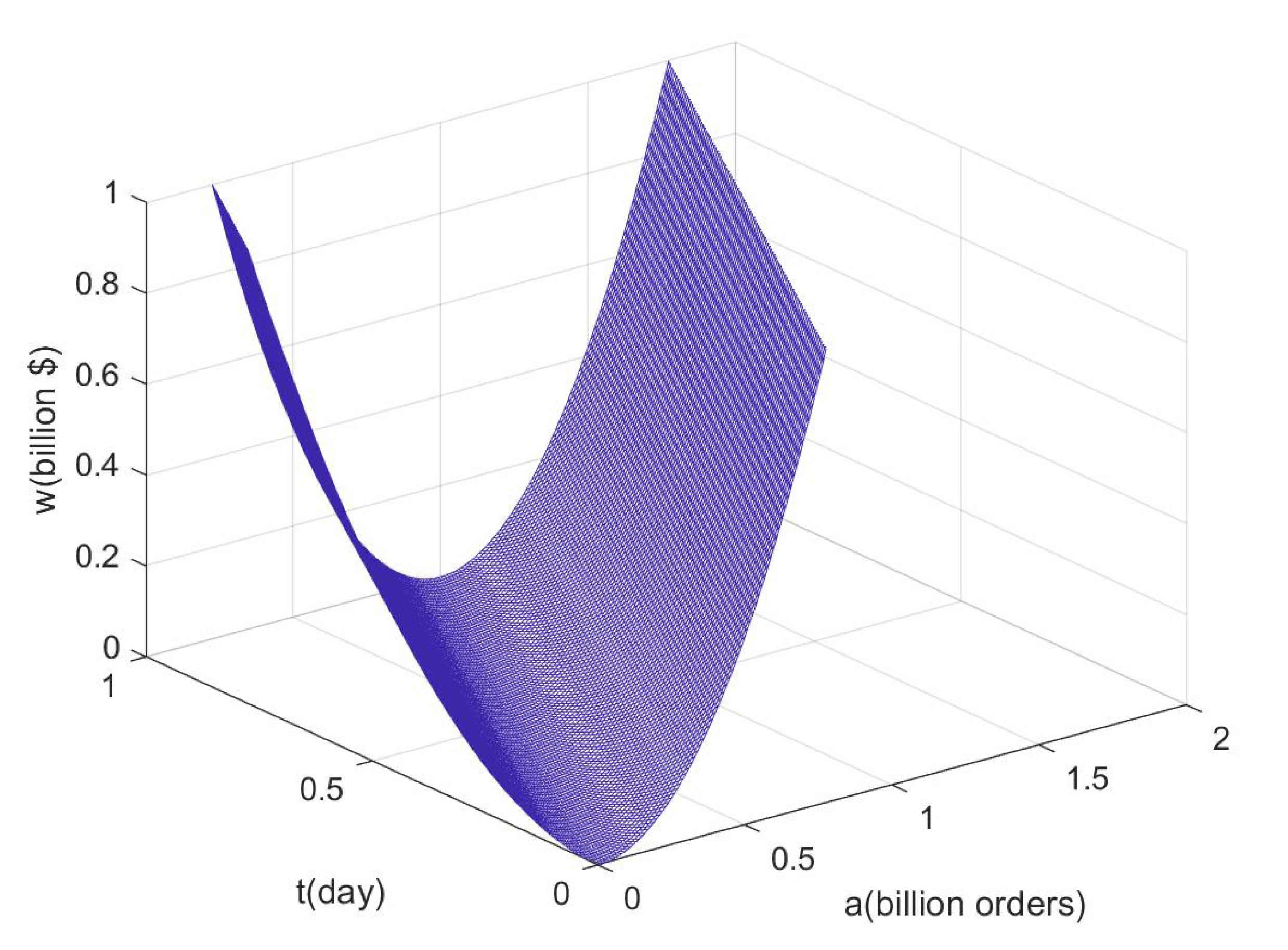
The following is the sensitivity analysis of the influence degree of A and T on W. The relation table of the change rate of W-a & t can be listed as Table 23 and Table 24. The W(max)-a and t diagram can be made as Figure 12.
As can be seen from the above tables and images, a and t have the same influence on the value of W while the influence is great. a changes by 20% near the base value, making the W change by about 25%. t changes by 33% near the base value, making the W change by about 25%.

6.3.3. Sensitivity Analysis of Factors Affecting the Income Allocation Pattern

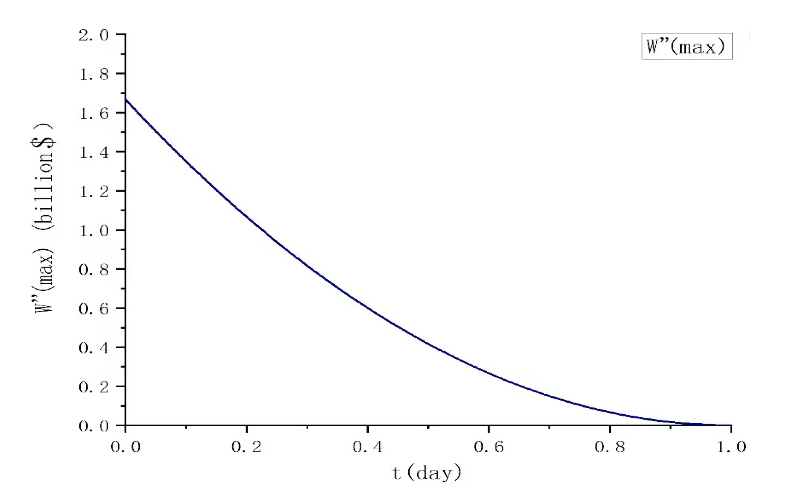
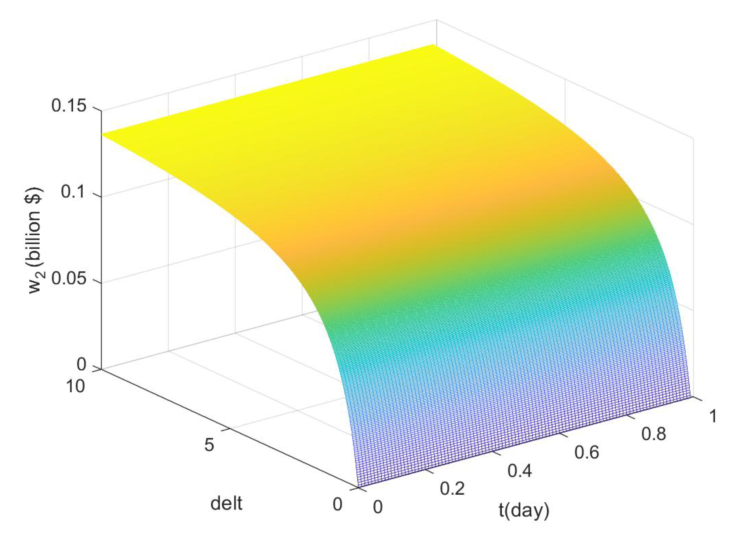
The W 1 (max)- δ , t diagram can be made as Figure 13. The W 2 (max)- δ , t diagram can be made as Figure 14. When the value of δ is different, the income of A and B are obviously different. It can be concluded that the value of δ has a great influence on the income allocation. With the change of δ , the changes of W 1 (max) and W 2 (max) can be shown in Table 25.
From the above analysis, it can be seen that:
When δ value is 0, the income proportion of A is 1, the income proportion of B is 0. As the value of δ changes from 0 to infinity, the income proportion of A decreases gradually, while the income proportion of B increases gradually. When the value of δ goes to infinity, the income proportion of B is 1, the income proportion of A is 0.

7. Conclusions

In this paper, we put forward a kind of logistics cooperative pattern named sharing logistics, put forward the cooperative pattern analysis model and the benefit distribution analysis model in sharing logistics, and combined them reasonably. In the analysis model of cooperative pattern, the judgment function is put forward, and the possible cooperative pattern is divided into three kinds by constructing and solving the replication dynamic equation. In the income allocation model, we proposed the game and income function considering the action sequence. At the same time, we connect the above two models, and the cooperation model analysis and benefit distribution model considering the multi-agent game situation are put forward. According to our research, logistics enterprises of different scales and with different characteristics can improve each other’s resource utilization rate and increase profits by joining "sharing logistics". However, this model still has some shortcomings, for example, it has not been tested by the complex transportation situation, and the research on the cooperative mode of mutual business is not in-depth enough. We will conduct further research in the future, and we expect this model to fully demonstrate its capability.

Author Contributions

Conceptualization, L.W.; Problem statement, G.P., H.J.; Data curation, H.J. and Q.J.; Model formulation, G.P., H.J., Q.J., T.Z. and J.W.; Model extension, H.J. and Q.J.; Example simulation, H.J., Q.J. and J.W.; Software, J.W.; Sensitivity analysis, H.J. and Q.J.; Original draft preparation, G.P. and H.J.; Writing, review and editing, H.J., Q.J. and G.P.; Visualization, J.W., H.J. and Q.J. All authors have read and agreed to the published version of the manuscript.

Funding

Not applicable.

Institutional Review Board Statement

Not applicable.

Informed Consent Statement

Not applicable.

Data Availability Statement

The data is available upon request from the corresponding author.

Acknowledgments

The authors would like to thank the journal editors for their constructive and valuable feedback.

Conflicts of Interest

The authors declare no conflict of interest.

References

  1. Acquier, A.; Daudigeos, T.; Pinkse, J. Promises and paradoxes of the sharing economy: An organizing framework. Technol. Forecast. Soc. Chang. 2017, 125, 1–10. [Google Scholar] [CrossRef]
  2. The State Information Center (Administration Center of China E-Government Network). Available online: http://www.sic.gov.cn/News/568/10429.htm (accessed on 11 June 2021).
  3. China Electronic Commerce Association (CECA). 2017–2018 E-commerce development report in China. Available online: http://www.100ec.cn/zt/upload_data/2018dzswfzbg.pdf (accessed on 15 March 2019).
  4. Klarin, A.; Suseno, Y. A state-of-the-art review of the sharing economy: Scientometric mapping of the scholarshi. J. Bus. Res. 2021, 126, 250–262. [Google Scholar] [CrossRef]
  5. Ferrell, O.C.; Ferrell, L.; Huggins, K. Seismic shifts in the sharing economy: Shaking up marketing channels and supply chains. J. Mark. Channels 2017, 24, 3–12. [Google Scholar] [CrossRef]
  6. Richter, C.; Kraus, S.; Brem, A.; Durst, S.; Giselbrecht, C. Digital entrepreneurship: Innovative business models for the sharing economy. Creat. Innov. Manag. 2017, 26, 300–310. [Google Scholar] [CrossRef]
  7. Clauss, T.; Harengel, P.; Hock, M. The perception of value of platform-based Business models in the sharing economy: Determining the drivers of user loyalty. Rev. Manag. Sci. 2019, 13, 605–634. [Google Scholar] [CrossRef]
  8. Belk, R. You are what you can access: Sharing and collaborative consumption online. J. Bus. Res. 2014, 7, 1595–1600. [Google Scholar] [CrossRef]
  9. Wang, J. Sharing logistics innovation model and development trend in China. Logist. Mater. Handl. 2017, 22, 80–84. [Google Scholar]
  10. Qin, X.; Liu, Z.; Tian, L. The strategic analysis of logistics service sharing in an e-commerce platform. Omega 2020, 92, 102153. [Google Scholar] [CrossRef]
  11. He, P.; Wen, J.; Ye, S.; Li, Z. Logistics service sharing and competition in a dual-channel e-commerce supply chain. Comput. Ind. Eng. 2020, 149, 106849. [Google Scholar] [CrossRef]
  12. Handoko, S.; Lau, H. Enabling carrier collaboration via order sharing double auction: A singapore urban logistics perspective. Transp. Res. Procedia 2016, 12, 777–786. [Google Scholar] [CrossRef] [Green Version]
  13. Wang, Y.; Zhang, J.; Guan, X.; Xu, M.; Wang, Z.; Wang, H. Collaborative multiple centers fresh logistics distribution network optimization with resource sharing and temperature control constraints. Expert Syst. Appl. 2021, 165, 113838. [Google Scholar] [CrossRef]
  14. Marcucci, E.; Pira, M.; Gatta, V.; Inturri, G.; Ignaccolo, M.; Pluchino, A. Simulating participatory urban freight transport policy-making: Accounting for heterogeneous stakeholders’ preferences and interaction effects. Transp. Res. Part E Logist. Transp. Rev. 2017, 103, 69–86. [Google Scholar] [CrossRef]
  15. He, P.; Zhang, S.; He, C. Impacts of logistics resource sharing on b2c e-commerce enterprises and customers. Electron. Commer. Res. Appl. 2019, 34, 100820. [Google Scholar] [CrossRef]
  16. Li, Y.; Liu, Y.; Liu, Y. An evolutionary game analysis of cooperation between high-speed rail express and express delivery enterprises. J. Railw. Sci. Eng. 2019, 16, 878–884. [Google Scholar]
  17. Luo, Y.; Wei, Q.; Gou, X.; Dai, D.; Zhou, Y. Sharing Logistics Service Supply Chain with Revenue-Sharing vs. Cost-Sharing Contracts. Math. Probl. Eng. 2021, 1024-123X, 8841536. [Google Scholar]
  18. Wong, L.H.M.; Davison, R.M. Knowledge sharing in a global logistics provider: An action research project. Inf. Manag. 2018, 55, 547–557. [Google Scholar] [CrossRef]
  19. Pham, H.; Nguyen, T.; Mcdonald, S.; Tran-Kieu, N. Information sharing in logistics firms: An exploratory study of thevietnamese logistics sector. Asian J. Shipp. Logist. 2019, 35, 87–95. [Google Scholar] [CrossRef]
  20. Khojasteh, M. A robust energy procurement strategy for micro-grid operator with hydrogen-based energy resources using game theory. Sustain. Cities Soc. 2020, 60, 102260. [Google Scholar] [CrossRef]
  21. Yang, C.; Lan, S.; Lin, T.; Wang, L.; Zhuang, Z.; Huang, G.Q. Transforming Hong Kong’s warehousing industry with a novel business model: A game-theory analysis. Robot. Comput. Integr. Manuf. 2020, 68, 102073. [Google Scholar] [CrossRef]
  22. Zhang, Y.; Chen, W.; Mi, Y. Third-party remanufacturing mode selection for competitive closed-loop supply chain based on evolutionary game theory. J. Clean. Prod. 2020, 263, 121305. [Google Scholar] [CrossRef]
  23. Bukvić, L.; Pašagić Škrinjar, J.; Abramović, B.; Zitrický, V. Route selection decision-making in an intermodal transport network using game theory. Sustainability 2021, 13, 4443. [Google Scholar] [CrossRef]
  24. Tatarczak, A. Profit allocation problems for fourth party logistics supply chain coalition based on game theory approach. J. Econ. Manag. 2018, 33, 120–135. [Google Scholar] [CrossRef]
  25. Friedman, D. Evolutionary games in economics. Econometrica 1991, 59, 637–666. [Google Scholar] [CrossRef] [Green Version]
  26. Xie, S. Economic Game Theory, 4th ed.; Fudan University Press: Shanghai, China, 2017; Volume 2, pp. 94–96. [Google Scholar]
  27. Kdhome (China Express Information Inquiry Platform). Available online: http://www.kiees.cn/freight/sto.htm (accessed on 11 June 2021).
Figure 1. Illustration of problem statement.
Sustainability 13 09347 g001
Figure 2. Bargaining game model.
Sustainability 13 09347 g002
Figure 3. Copy dynamic phase diagram of sixteen situations.
Sustainability 13 09347 g003
Figure 4. Two situations (I,II) in Multi-enterprise cooperation model illustration.
Sustainability 13 09347 g004
Figure 5. W(max)-t relational figure.
Sustainability 13 09347 g005
Figure 6. W 1 (max)-t relational figure.
Sustainability 13 09347 g006
Figure 7. W 2 (max)-t relational figure.
Sustainability 13 09347 g007
Figure 8. W 1 (max)-t relational figure.
Sustainability 13 09347 g008
Figure 9. W 2 (max)-t relational figure.
Sustainability 13 09347 g009
Figure 10. W (max)-t relational figure.
Sustainability 13 09347 g010
Figure 11. p-a, t diagram of sensitivity analysis.
Sustainability 13 09347 g011
Figure 12. W(max)-a, t diagram of sensitivity analysis.
Sustainability 13 09347 g012
Figure 13. W 1 (max)- δ , t diagram of sensitivity analysis.
Sustainability 13 09347 g013
Figure 14. W 2 (max)- δ , t diagram of sensitivity analysis.
Sustainability 13 09347 g014
Table 1. Main notations and corresponding explanations.
NotationDefinitionDescription
ALogistics enterprise AGame subject 1
BLogistics enterprise BGame subject 2
YCooperation pattern is cooperationGame strategy 1
NCooperation pattern is not cooperationGame strategy 2
xProbability of logistics enterprise A
adopting cooperation
0 ≤ x ≤ 1
yProbability of logistics enterprise B
adopting cooperation
0 ≤ y ≤ 1
π 1 In the state of non-cooperation between the two
parties, the overall profit of A from operating its
own business
π 1 ≥ 0
π 2 In the state of non-cooperation between the two
parties, the overall profit of B from operating its
own business
π 2 ≥ 0
π 1 When A and B cooperate in two ways,
the overall profit of A
π 1 ∈ R
π 2 When A and B cooperate in two ways,
the overall profit of B
π 2 ∈ R
π 3 When A unilaterally shares resources
with B, the overall profit of A
π 3 ∈ R
π 4 When A unilaterally shares resources
with B, the overall profit of B
π 4 ∈ R
π 5 When B unilaterally shares resources
with A, the overall profit of A
π 5 ∈ R
π 6 When B unilaterally shares resources
with A, the overall profit of B
π 6 ∈ R
π 7 When A and B fail to cooperate,
the overall profit of A
π 7 ∈ R
π 8 When A and B fail to cooperate,
the overall profit of B
π 8 ∈ R
Table 2. Negotiation cost ratio coefficient of enterprise A and B (nc 1 nc 4 < nc 3 < nc 2 ).
Negotiation Cost RatioEnterprise B
Share ResourcesNot Share Resources
Enterprise AShare resourcesnc 1 , 1 − nc 1 nc 2 , 1 − nc 2
Not share resourcesnc 3 , 1 − nc 3 nc 4 , 1 − nc 4
Table 3. Parameter setting.
NotationDefinitionDescription
p 1 The price of each express which A helps B
to transport
p 1 > 0
p 2 The price of each express which B helps A
to transport
p 2 > 0
s 1 The market price of each express of As 1 > 0
s 2 The market price of each express of Bs 2 > 0
m 1 The number of express transported with own
transportation resources of A
m 1 > 0
m 2 The number of express transported with own
transportation resources of B
m 2 > 0
n 1 The number of express transported for the
counterparty of A
n 1 > 0
n 2 The number of express transported for the
counterparty of B
n 2 > 0
bThe total risk cost of Ab > 0
b The total risk cost of Bb > 0
ncNegotiation cost ratio coefficient0 < nc 1 nc 4 < nc 3 < nc 2 < 1
cAverage negotiation cost under different
cooperation states
c > 0
Table 4. Negotiation cost ratio coefficient of enterprise A and B (nc 1 nc 4 < nc 3 < nc 2 ).
Negotiation Cost RatioEnterprise B
Share ResourcesNot Share Resources
Enterprise AShare resources π 1 , π 2 π 3 , π 4
Not share resources π 5 , π 6 π 7 , π 8
Table 5. Parameter setting.
ParameterDefinition
WThe overall income
aAnnual orders in the first-tier city market
tThe average transportation time
pThe average freight
k 1 User’s perception coefficient of transportation time
k 2 User’s perception coefficient of freight
QThe order quantity function
Table 6. Bargaining game model parameter setting.
ParameterDefinition
W 1 The share of the income of A in Pattern 1
W 2 The share of the income of B in Pattern 1
W 1 The share of the income of A in Pattern 2
W 2 The share of the income of B in Pattern 2
W 1 The share of the income of A in Pattern 3
W 2 B’s share of the income of B in Pattern 3
δ The proportion of orders lost after each bargaining round
Table 7. Local stability analysis results I.
Equilibrium
Point
π 1 π 5 < 0 π 1 π 5 < 0 π 1 π 5 < 0
π 2 π 4 < 0 π 2 π 4 < 0 π 2 π 4 < 0
π 3 π 7 < 0 π 3 π 7 < 0 π 3 π 7 > 0
π 6 π 8 < 0 π 6 π 8 > 0 π 6 π 8 < 0
Det(J)tr(J)StabilityDet(J)tr(J)StabilityDet(J)tr(J)Stability
(0,0)+ESSuncertainSaddle
point
uncertain
point
(0,1)uncertainSaddle
point
+ESSuncertainSaddle
point
(1,0)uncertainSaddle
point
uncertainSaddle
point
+ESS
(1,1)++Unstable++Unstable++Unstable
Table 8. Local stability analysis results II.
Equilibrium
Point
π 1 π 5 < 0 π 1 π 5 < 0 π 1 π 5 < 0
π 2 π 4 < 0 π 2 π 4 < 0 π 2 π 4 < 0
π 3 π 7 < 0 π 3 π 7 < 0 π 3 π 7 > 0
π 6 π 8 < 0 π 6 π 8 > 0 π 6 π 8 < 0
Det(J)tr(J)StabilityDet(J)tr(J)StabilityDet(J)tr(J)Stability
(0,0)++Unstable+EESuncertainSaddle
point
(0,1)UnstableuncertainSaddle
point
+EES
(1,0)+EES++Unstable++ESS
(1,1)++UnstableuncertainSaddle
point
uncertainSaddle
point
Table 9. Local stability analysis results III.
Equilibrium
Point
π 1 π 5 < 0 π 1 π 5 < 0 π 1 π 5 < 0
π 2 π 4 < 0 π 2 π 4 < 0 π 2 π 4 < 0
π 3 π 7 < 0 π 3 π 7 < 0 π 3 π 7 > 0
π 6 π 8 < 0 π 6 π 8 > 0 π 6 π 8 < 0
Det(J)tr(J)StabilityDet(J)tr(J)StabilityDet(J)tr(J)Stability
(0,0)uncertainSaddle
point
++Unstable+ESS
(0,1)uncertainSaddle
point
+EES++Unstable
(1,0)uncertainSaddle
point
uncertainSaddle
point
uncertainSaddle
point
(1,1)uncertainSaddle
point
uncertainSaddle
point
uncertainSaddle
point
Table 10. Local stability analysis results IV.
Equilibrium
Point
π 1 π 5 < 0 π 1 π 5 < 0 π 1 π 5 < 0
π 2 π 4 < 0 π 2 π 4 < 0 π 2 π 4 < 0
π 3 π 7 < 0 π 3 π 7 < 0 π 3 π 7 > 0
π 6 π 8 < 0 π 6 π 8 > 0 π 6 π 8 < 0
Det(J)tr(J)StabilityDet(J)tr(J)StabilityDet(J)tr(J)Stability
(0,0)uncertainSaddle
point
uncertainSaddle
point
++Unstable
(0,1)uncertainSaddle
point
++UnstableuncertainSaddle
point
(1,0)uncertainSaddle
point
+EES+EES
(1,1)uncertainSaddle
point
uncertainSaddle
point
uncertainSaddle
point
Table 11. Local stability analysis results V.
Equilibrium
Point
π 1 π 5 < 0 π 1 π 5 < 0 π 1 π 5 < 0
π 2 π 4 < 0 π 2 π 4 < 0 π 2 π 4 < 0
π 3 π 7 < 0 π 3 π 7 < 0 π 3 π 7 > 0
π 6 π 8 < 0 π 6 π 8 > 0 π 6 π 8 < 0
Det(J)tr(J)StabilityDet(J)tr(J)StabilityDet(J)tr(J)Stability
(0,0)UnstableuncertainSaddle
point
uncertainSaddle
point
(0,1)++UnstableuncertainSaddle
point
++Unstable
(1,0)++Unstable++UnstableuncertainSaddle
point
(1,1)+ESS+ESS+ESS
Table 12. Local stability analysis results VI.
Equilibrium Point π 1 π 5 > 0
π 2 π 4 > 0
π 3 π 7 < 0
π 6 π 8 < 0
Det(J)tr(J)Stability
(0,0)++Unstable
(0,1)uncertainSaddle point
(1,0)uncertainSaddle point
(1,1)+ESS
Table 13. Parameter assignment I.
ParameterEvaluation
p 1 USD 12
p 2 USD 10
S 1 USD 18
S 2 USD 14
b 1 USD 560,000
b 2 USD 560,000
nc 1 0.5
CUSD 300,000
m 1 600,000
m 2 700,000
n 1 400,000
n 2 100,000
Table 14. Parameter assignment II.
Parameter UnitEvaluation
a (billion orders)1
k 1 (billion orders/day)1
k 2 (billion orders/USD)0.15
δ 0.95
Table 15. W(max)-p/t relational table.
t (day)p (USD)W(max)(billion USD)
0.22.671.07
0.42.000.60
0.61.330.27
0.80.670.07
Table 16. W 1 (max)-t relational table.
t (day)W 1 (max)(billion USD)
0.20.55
0.40.31
0.60.14
0.80.03
Table 17. W 2 (max)-t relational table.
t (day)W 2 (max)(billion USD)
0.20.52
0.40.29
0.60.13
0.80.03
Table 18. W 1 (max)-t relational table.
t (day)W 1 (max)(billion USD)
0.20.52
0.40.29
0.60.13
0.80.03
Table 19. W 2 (max)-t relational table.
t (day)W 2 (max)(billion USD)
0.20.55
0.40.31
0.60.14
0.80.03
Table 20. W (max)-t relational table.
t (day)p (USD)W (max)(billion USD)
0.22.671.07
0.42.000.60
0.61.330.27
0.80.670.07
Table 21. The rate of change of p-a relational.
a (billion Orders)The Rate of Change of ap (USD)The Rate of Change of p
0.6−40.00%0.00100.00%
0.8−20.00%0.67−49.87%
1 (base value)0.00%1.330.00%
1.220.00%2.0050.38%
1.440.00%2.67100.00%
Table 22. The rate of change of p-t relational.
t (day)The Rate of Change of tp (USD)The Rate of Change of p
0.2−66.67%2.67100.00%
0.4−33.33%2.0050.38%
0.6 (base value)0.00%1.330.00%
0.833.33%0.67−49.87%
166.67%0.00−100.00%
Table 23. The rate of change of W-a relational.
a (Billion Orders)The Rate of Change of aW (billion USD)The Rate of Change of W
0.6−40.00%0.00−100.00%
0.8−20.00%0.07−75.31%
1 (base value)0.00%0.270
1.220.00%0.60122.22%
1.440.00%1.07295.06%
Table 24. The rate of change of W-t relational.
t (day)The Rate of Change of tW (billion USD)The Rate of Change of W
0.2−66.67%1.07295.06%
0.4−33.33%0.60122.22%
0.6 (base value)0.00%0.270
0.833.33%0.07−75.31%
166.67%0.00−100.00%
Table 25. δ - W 1 (max)/W 2 (max) income allocation.
δ W 1 (max)W 2 (max)
010
0.283.33%16.67%
0.471.43%28.57%
0.662.50%37.50%
0.855.56%44.44%
150.00%50.00%
109.09%90.91%
1000.99%99.01%
10000.10%99.90%
01
Publisher’s Note: MDPI stays neutral with regard to jurisdictional claims in published maps and institutional affiliations.