An Ensemble 3D Convolutional Neural Network for Spatiotemporal Soil Temperature Forecasting

Abstract

Soil temperature (ST) plays an important role in agriculture and other fields, and has a close relationship with plant growth and development. Therefore, accurate ST prediction methods are widely needed. Deep learning (DL) models have been widely applied for ST prediction. However, the traditional DL models may fail to capture the spatiotemporal relationship due to its complex dependency under different related hydrologic variables. Hence, the DL models with Ensemble Empirical Mode Decomposition (EEMD) are proposed in this study. The proposed models can capture more complex spatiotemporal relationship after decomposing the ST into different intrinsic mode functions. Therefore, the performance of models is further improved. The results show that the performance of DL models with EEMD are better than that of corresponding DL models without EEMD. Moreover, EEMD-Conv3d has the best performance among all the experimental models. It has the highest R2 ranging from 0.9826 to 0.9893, the lowest RMSE ranging from 1.3096 to 1.6497 and the lowest MAE ranging from 0.9656 to 1.2056 in predicting ST at the lead time from one to five days. In addition, the lines between predicted ST and observed ST are closer to the ideal line (y = x) than other DL models. The results show that our EEMD-Conv3D can better capture spatiotemporal correlation and is an applicable method for predicting spatiotemporal ST.

1. Introduction

Soil temperature (ST) is one of the most important factors affecting the processes of soil properties involved in plant growth [1,2,3,4]. It controls physical, chemical, and biological processes in soil and influences plant growth, development, and soil formation. In agriculture, ST plays an important role because it is one of the factors that contribute to seed germination, and most soil organisms need to function at optimal soil temperature. ST also affects the rate of nitrification, soil water content, vent ability, and availability of plant nutrients. In addition, various biochemical processes in soil, such as those caused by microbial activity and non-living chemical processes, are also influenced by ST. Therefore, ST prediction is of great importance. Usually, prediction methods are mainly focus on the time-based temperature series of a site, but spatiotemporal ST prediction has been little studied. In this paper, we investigate a method for predicting spatiotemporal soil temperature.

For ST prediction at one point site and similar time series prediction, statistical models and machine learning models are usually applied [5,6,7,8]. The commonly used statistical models are Box-Jenkins models, including ARMA and ARIMA [9]. For examples, Shirvani et al. [10] predicted the ST anomalies at one grid point using ARIMA model and Chen et al. [11] forecasted the short-term load of a power system by an adaptive ARMA model. After this, the most widely applied models for time-series prediction are machine learning, including artificial neural network (ANN), support vector regression (SVR), etc. Mihalakakou [12] used a neural network approach to predict surface soil temperature. Lekkas et al. [13] proposed an application of ANNs to make predictions of floods. Abdel-Aal [14] proposed abductive networks and achieved hourly temperature forecasting. Bilgili [15] compared ANN with linear regression (LR) and nonlinear regression (NLR) in predicting monthly ST and proved that ANN has better performance than LR and NLR. Tabari [16] used air temperature and ST as inputs to ANN and realized ST prediction at different depths over one site. Salcedo-Sanz et al. [17] used SVR to achieve predictions of long-term air temperature over Australian and New Zealand observational stations. Kisi [18] compared the performance of ANN, adaptive neuro-fuzzy inference system (ANFIS), and genetic programming (GP) in predicting monthly ST and showed that ANN can better use the data from nearby sites for prediction. Delbari [19] used SVR to predict daily ST and showed that SVR was effective in predicting deep ST. Recently, DL models provide some useful insights on solving this problem, especially recurrent neural network (RNN) and long short-term memory (LSTM) models. For examples, Tokgoz et al. [20] tested RNN and LSTM on electricity consumption prediction and proved that they have better results than ANN and ARIMA. Hewage [21] used LSTM to achieve efficient and accurate prediction of numerical weather forecasts through time series data of weather information. Although methods are capable of making predictions based on time series. When predictions are made for spatiotemporal ST data, these methods become a little inapplicable. Traditional DL models such as ANN and LSTM cannot guarantee the relationship of data information in temporal and spatial dimensions at the same time. These methods of discarding some information will reduce the accuracy of prediction. To capture the information of the data in both temporal and spatial dimensions, convolution operators are required. Two-dimensional convolutional neural networks (Conv2D) are suitable for image processing [22], and they are able to preserve features in temporal dimension on channels. Three-dimensional convolutional neural networks (Conv3D) are applicable in the field of video processing [23,24], and 3D convolutional kernels are able to slide in the temporal dimension, to preserve the temporal information of the input data. In addition to them, Convolutional LSTM Network (ConvLSTM) [25] is also applicable to spatiotemporal data in three dimensions. Compared with the traditional LSTM [7], Shi et al. replaces the point multiplication in LSTM cell with convolution operations, so that the two-dimensional spatial data can be used as the input of LSTM cells instead of one-dimensional inputs that drops some spatial information. Hence, in this paper, we test Conv2D, Conv3D and ConvLSTM models for predicting spatiotemporal ST.

Ensemble empirical mode decomposition (EEMD) is an adaptive decomposition method for time series processing proposed by Wu and Huang [26], and many models combined with EEMD have been successfully applied in several fields. For example, Wang et al. [27] combined ARIMA with EEMD to predict annual runoff prediction, Zhang et al. [28] combined multidimensional k-nearest neighbor model with EEMD to forecast closing price and high price of stocks, Zhang et al. [29] combined LSTM with EEMD to predict land surface temperature. After combining EEMD, the accuracy of the prediction models all significantly improved. The IMFs obtained from time series decomposed by EEMD can show more variation patterns of the original time series. EEMD decomposes ST into features in different modalities that reflect the trend of ST in different situations, thus converting complex patterns of ST into simple patterns in different modalities helps DL models to learn the complex nonlinear relationships of ST and further improve prediction performance of each DL model. Hence, in this paper, we combine EEMD with three DL models, Conv2D, Conv3D and ConvLSTM, to compare prediction performance of the models after combining EEMD. The results show that the performance of the DL models are significantly improved after combining with EEMD, and EEMD-Conv3D has the best prediction performance.

2. Materials and Methods

2.1. Experimental Data

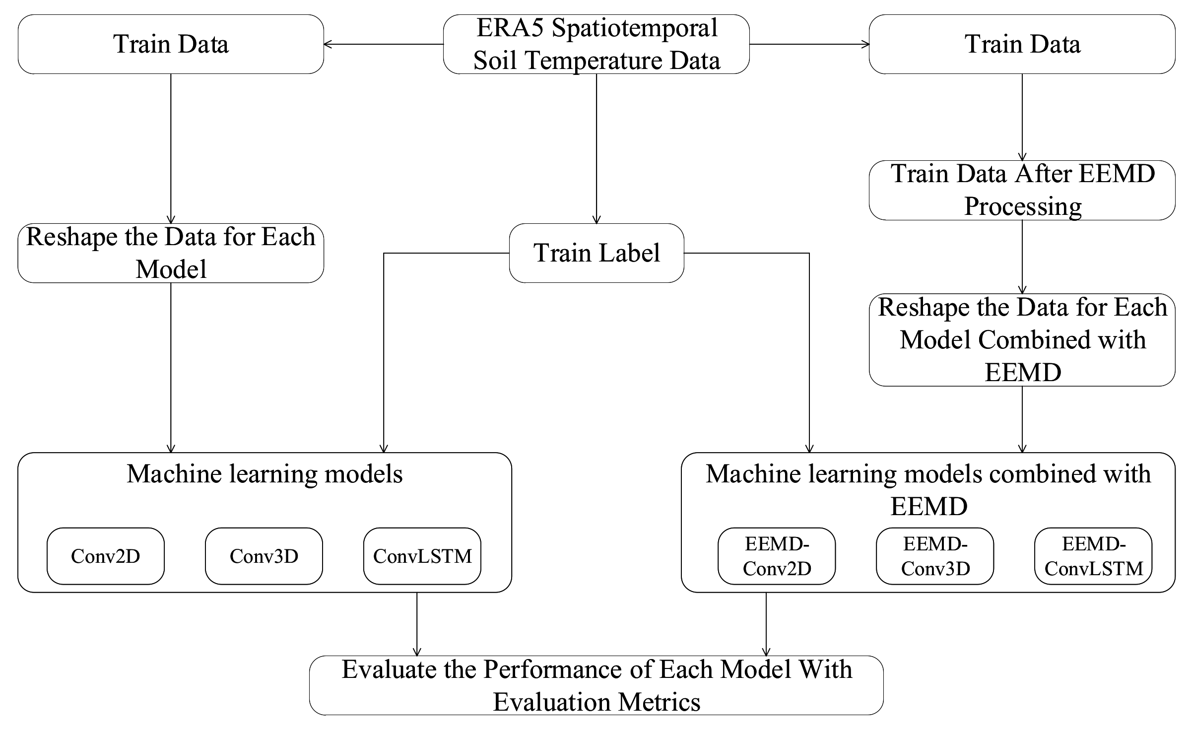
The study area (33° N–52° N, 112° E–131° E) (Figure 1) of this paper mainly covers the northeast part of China. The experimental dataset is ERA5 which is downloaded from Climate Data Store (https://cds.climate.copernicus.eu/, accessed on 27 February 2021) on a daily time scale. We used layer 1 (0–7 cm) soil temperature of ERA5 dataset to test models on predicting spatiotemporal ST. The ST data from ERA5 has units of kelvin (K), we converted it to degrees Celsius (°C) by subtracting 273.15. The data we used is from 6 July 2012 to 22 September 2020, a total of 3000 days of data, each day’s data are made up of 400 grids (20 × 20). We divided the selected area equally into four areas and calculated the statistical characteristics of each area separately. The statistical characteristics of ST in each area are shown in

Table 1. The Statistical characteristics of the ERA5 dataset in the experimental area.

Data	Minimum	Maximum	Mean	Median	Standard Deviation
Northwest Area (43° N–52° N, 112° E–121° E)	−37.071	30.835	0.764	0.709	13.616
Northeast Area (43° N–52° N, 122° E–131° E)	−35.452	29.477	2.967	2.477	12.952
Southwest Area (33° N–42° N, 112° E–121° E)	−28.354	33.745	11.017	11.944	10.918
Southeast Area (33° N–42° N, 122° E–131° E)	−27.582	32.727	13.325	14.582	9.462
Overall (33° N–52° N, 112° E–131° E)	−37.071	33.745	7.018	9.056	12.973

. The northwest area with a predominantly temperate continental climate has a high standard deviation and the ocean-dominated southeast area has a low standard deviation. The standard deviations of the remaining two areas with predominantly temperate monsoonal climate are between the above two areas. It shows that areas near the ocean have less variation in ST.

2.2. Methods

2.2.1. Ensemble Empirical Mode Decomposition (EEMD)

Empirical mode decomposition (EMD) is a method for processing signals proposed by Huang et al. [30,31]. It is capable of adaptively decomposing a complex signal into a series of intrinsic mode functions (IMFs) according to the characteristics of the signal. The decomposed IMF contains local characteristic signals of the original signal at different time scales. The essence of EMD is to identify all the intrinsic oscillation modes contained in the signal by the characteristic time scales. EMD is adaptive because it is based on the local characteristics of the signal sequence time scales.

EMD decomposes the original signal into IMFs by the following steps:

• Find all extreme value points of the signal x (t).
• Fit the envelopes emax (t) and emin (t) of the upper and lower extremal points with cubic spline fitting and find the average of two envelope lines m (t), then subtract m (t) in x (t):h (t) = x (t) − m (t).
• Determine whether h (t) is IMF according to the preset criterion.
• If not, replace x (t) with h (t) and repeat the above steps until h (t) satisfies the criterion, then h (t) is the IMF Ck (t) to be extracted.
• Every time an IMF is obtained, it is subtracted from the original signal, and the above steps are repeated; until the last remaining part of the signal rn (t) is just a monotonic sequence or a constant value sequence.

In this way, the decomposition by the EMD method decomposes the original signal x (t) into series of IMFs and a linear superposition of the remaining parts as Equation (1):

$$x\left(t\right)=\sum _{k=0}^N{C}_k\left(t\right)+r_n\left(t\right)$$

(1)

Despite EMD has good performance in decomposing signals, EMD also has some problems and drawbacks, such as endpoint effect and mode mixing. The endpoint effect refers to the fact that different treatments of endpoints will bring different results in the EMD decomposition process, while the mode mixing may cause severe mixing of time-frequency distribution and lead to degradation of decomposition accuracy. On the basis of EMD, Huang and WU then proposed the ensemble empirical mode decomposition (EEMD) [26].

EEMD is a signal decomposition method to improve EMD by adding white noise to the EMD method. The principle of EEMD is that extreme values of the signal affect IMFs. In addition, if the distribution is not uniform, there will occur mode mixing. EEMD introduces white noise into the signal to be analyzed, the spectrum of white noise is uniformly distributed, and white noise makes the signal automatically distributed to a suitable reference scale. Due to the characteristics of zero-mean noise, the effect of noise will be offset after several averaging calculations, so that the integrated average calculation can be directly regarded as the final result. The process of EEMD can be described as follows:

• Add normally distributed white noise to the original signal.
• The signal with white noise is taken as a whole and decomposed into IMF using EMD.
• Repeat the previous steps, adding a different sequence of normally distributed white noise to the original signal each time.
• The IMF obtained each time will be integrated and averaged as the final result.

Compared with Fourier transform, wavelet decomposition and other methods, EMD has the advantages of principal component analysis, adaptive time-frequency analysis and signal local transient characterization. In addition, EEMD also overcomes the problems of endpoint effects and mode mixing in EMD, so we use EEMD to process ST data on the time scale.

2.2.2. Convolutional Neural Network (CNN)

CNN is a feed-forward neural network that includes convolutional computation and is one of the representative algorithms of DL. It is often used for image recognition, image classification, and natural language processing. In addition, CNN is also used in remote sensing science and atmospheric science. In atmospheric science, CNN is used in post-processing problems for numerical pattern lattice point outputs. In remote sensing science, especially in satellite remote sensing. CNN is considered to have advantages in computational efficiency and classification accuracy in resolving geometric, textural, and spatially distributed features of remote sensing images. Therefore, in this paper we use two kinds of convolutional neural networks, Conv2d and Conv3d, to predict spatiotemporal ST. Conv2d is commonly used in computer vision, image processing [22,32,33,34]. In addition, Conv3d is commonly used in the medical field (CT imaging), video processing and other fields [24,35].

The difference between Conv2D and Conv3D is shown in Figure 2. In Conv2d, a two-dimensional convolution kernel slides in the spatial dimension to extract higher-order features from the input data (Batch*Height *Width*Channels). The channels of the input data correspond to sequences of soil temperatures in the temporal dimension over consecutive days or the sequences obtained after EEMD processing. In Conv3d, the three-dimensional convolution kernel slides not only in the spatial dimension, but also in the temporal dimension. Therefore, it can better handle the features of the input data (Batch*Depth*Height*Width*Channels) in the temporal dimension. The channels of the input data correspond to one-day ST in the time dimension or a one-day sequence after EEMD processing.

2.2.3. Convolutional LSTM Network (ConvLSTM)

Long short-term memory network (LSTM) is a kind of temporal recurrent neural network, which is especially designed to solve long-term dependence problem of general recurrent neural network (RNN). LSTM is suitable for processing and predicting events with very long intervals and delays in time series. LSTM has achieved good results in fields of speech recognition, video analysis, sequence modeling [36], etc. The traditional LSTM network consists of five modules: input gate i_t, forget gate f_t, output gate o_t, cell output ct and hidden state h_t five modules, x_t denotes the input of LSTM, and the relationship between them can be represented as Equations (2)–(6), where ‘∘’ denotes the Hadamard product:

$$\begin{array}{cc}\hfill & i_t=\sigma (W_{xi}{x}_t+W_{hi}{h}_{t-1}+W_{ci}\circ c_{t-1}+b_i)\hfill \end{array}$$

(2)

$$\begin{array}{cc}\hfill & f_t=\sigma (W_{xf}{x}_t+W_{hf}{h}_{t-1}+W_{cf}\circ c_{t-1}+b_f)\hfill \end{array}$$

(3)

$$\begin{array}{cc}\hfill & c_t=f_t\circ c_{t-1}+i_t\circ tanh(W_{xc}{x}_t+W_{hc}{h}_{t-1}+b_c)\hfill \end{array}$$

(4)

$$\begin{array}{cc}\hfill & o_t=\sigma (W_{xo}{x}_t+W_{ho}{h}_{t-1}+W_{co}\circ c_t+b_o)\hfill \end{array}$$

(5)

$$\begin{array}{cc}\hfill & h_t=o_t\circ tanh\left(c_t\right)\hfill \end{array}$$

(6)

Although traditional LSTM has proven to be powerful in dealing with temporal correlation, it contains too much redundancy for spatial data. To solve this problem, Xingjian Shi proposed an extension to the traditional LSTM, the Convolutional LSTM Network. In the ConvLSTM, there are convolutional structures in both the input-to-state and state-to-state transitions. Therefore, ConvLSTM overcomes the drawback of traditional LSTM that uses full connections in the input-to-state and state-to-state transitions while processing spatiotemporal data, resulting in spatial information not being encoded. When using convolution operators to process input-to-state and state-to-state transitions, the future state of a cell in the grid will be determined by the input and past state of its local neighbors. The equations of ConvLSTM are shown as Equations (7)–(11), where ‘∗’ denotes the convolution operator and ‘∘’ denotes the Hadamard product. To distinguish the tensor of different dimensions from the traditional LSTM, Xt, Ct, Ht denote the input, cell output and hidden state respectively:

$$\begin{array}{cc}\hfill & i_t=\sigma (W_{xi}\ast X_t+W_{hi}\ast H_{t-1}+W_{ci}\circ C_{t-1}+b_i)\hfill \end{array}$$

(7)

$$\begin{array}{cc}\hfill & f_t=\sigma (W_{xf}\ast X_t+W_{hf}\ast H_{t-1}+W_{cf}\circ C_{t-1}+b_f)\hfill \end{array}$$

(8)

$$\begin{array}{cc}\hfill & C_t=f_t\circ C_{t-1}+i_t\circ tanh(W_{xc}\ast X_t+W_{hc}\ast H_{t-1}+b_c)\hfill \end{array}$$

(9)

$$\begin{array}{cc}\hfill & o_t=\sigma (W_{xo}\ast X_t+W_{ho}\ast H_{t-1}+W_{co}\circ C_t+b_o)\hfill \end{array}$$

(10)

$$\begin{array}{cc}\hfill & H_t=o_t\circ tanh\left(C_t\right)\hfill \end{array}$$

(11)

Just like the dimensionality as the input data of Conv3d, input data of ConvLSTM is also a 5D tensor (Batch*Timestep*Height*Width*Channels). The input of the neural network module in ConvLSTM is the data in one timestep. For a video, data in one timestep can be interpreted as a video frame. In our experiments, data in one timestep is ST data in spatial dimension.

2.2.4. Model Training and Test

In this study, the original spatiotemporal data and the EEMD processed spatiotemporal data are used to train Conv2d, Conv3d and Conv-LSTM models to predict soil temperatures one day later, three days later and five days later. Persistent forecasting (PF) [37] is also involved in the comparison, which is a simple forecasting method that treats the first day’s temperature as the next day’s forecast. PF can be seen as a minimum criterion to assess the feasibility of DL methods. Experimental data will be split into two parts. The first part, including 80% data, is used for training models. The remaining 20% data are used as the testing set. The overall flow of the experiment is shown in Figure 3.

In the process of training models, we use 10 consecutive days of spatiotemporal ST data to predict the ST after 1, 3 and 5 days in the future. When raw ST data are input into Conv3D and ConvLSTM, there is only 1 channel in the data, where the value is the ST value for a specific area on a particular day. When using EEMD to process ST data, EEMD decomposes the ST sequence in the temporal dimension for the ST in each grid. We set the number of IMFs manually. So the temperature sequence of a certain area was processed by EEMD to obtain 9 IMFs and 1 residual sequence. There are 10 channels of input in EEMD-Conv3D and EEMD-ConvLSTM. For Conv2D, the input tensor can only cover the spatial dimension, so continuous sequences about the ST in the time dimension are preserved through the channels. Therefore, the input data of Conv2D has 10 times more channels than the other two models. The parameter settings of each model are shown in

Table 2. The parameter settings of each model.

Models	Input Size	Kernel Size	Strides
Conv2D	(20,20,10)	3 × 3	(1,1)
Conv3D	(10,20,20,1)	(5,2,2,3) × 3 × 3	[(1,2,2,3),1,1]
ConvLSTM	(10,20,20,1)	3 × 3	(1,1)
EEMD-Conv2D	(20,20,100)	3 × 3	(1,1)
EEMD-Conv3D	(10,20,20,10)	(5,2,2,3) × 3 × 3	[(1,2,2,3),1,1]
EEMD-ConvLSTM	(10,20,20,10)	3 × 3	(1,1)

.

To evaluate the above models and compare their performance in predicting spatiotemporal ST, several statistical evaluation metrics including mean absolute error (MAE), mean squared error (MSE), root mean square error (RMSE), r-squared ($R^2$) and mean absolute percentage error (MAPE) are applied to assess model performance. The evaluation metrics are defined as Equation (12) to Equation (16) (yi is the true value of the testing set, ŷi is the prediction value of the model). Due to the existence of division in the calculation of MAPE, the minimum absolute value of the true value is 0.02189 ${}^{\circ }$C. Such kind of data that is close to 0 ${}^{\circ }$C will seriously affect the accuracy of MAPE. Therefore, we averaged the 400 grids of each day before calculating MAPE.

$$\begin{array}{cc}\hfill & MAE=\frac{{\sum }_{i=1}^n\left|y_i-{\widehat{y}}_i\right|}{n}\hfill \end{array}$$

(12)

$$\begin{array}{cc}\hfill & MSE=\frac{{\sum }_{i=1}^n{(y_i-{\widehat{y}}_i)}^2}{n}\hfill \end{array}$$

(13)

$$\begin{array}{cc}\hfill & RMSE=\sqrt{\frac{{\sum }_{i=1}^n{(y_i-{\widehat{y}}_i)}^2}{n}}\hfill \end{array}$$

(14)

$$\begin{array}{cc}\hfill & R^2=1-\frac{{\sum }_{i=1}^n{(y_i-{\widehat{y}}_i)}^2}{{\sum }_{i=1}^n{(y_i-{\overline{y}}_i)}^2}\hfill \end{array}$$

(15)

$$\begin{array}{cc}\hfill & MAPE=\sum _{i=1}^n\left|\frac{y_i-{\widehat{y}}_i}{y_i}\right|\times \frac{100\%}{n}\hfill \end{array}$$

(16)

3. Results and Discussion

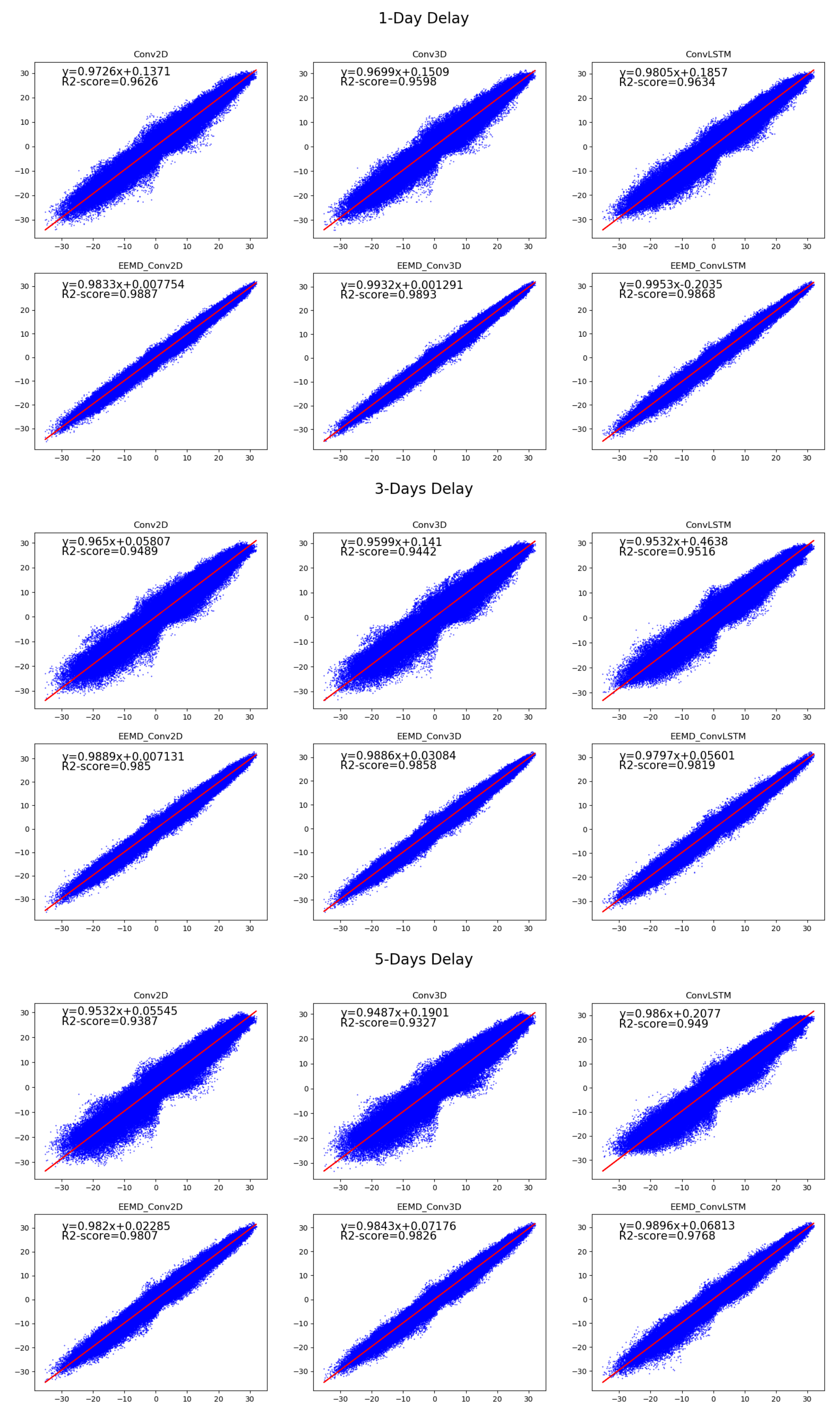
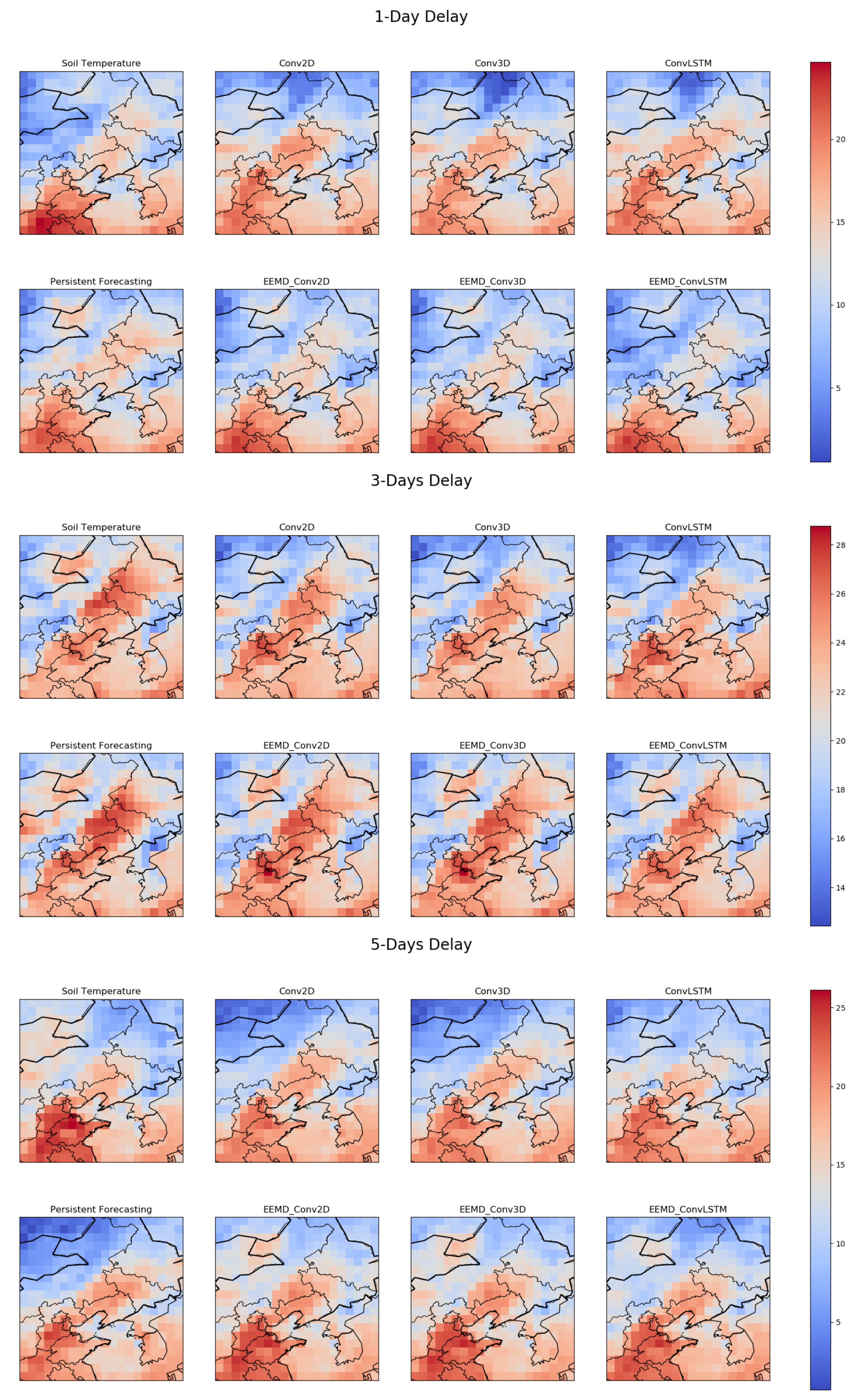
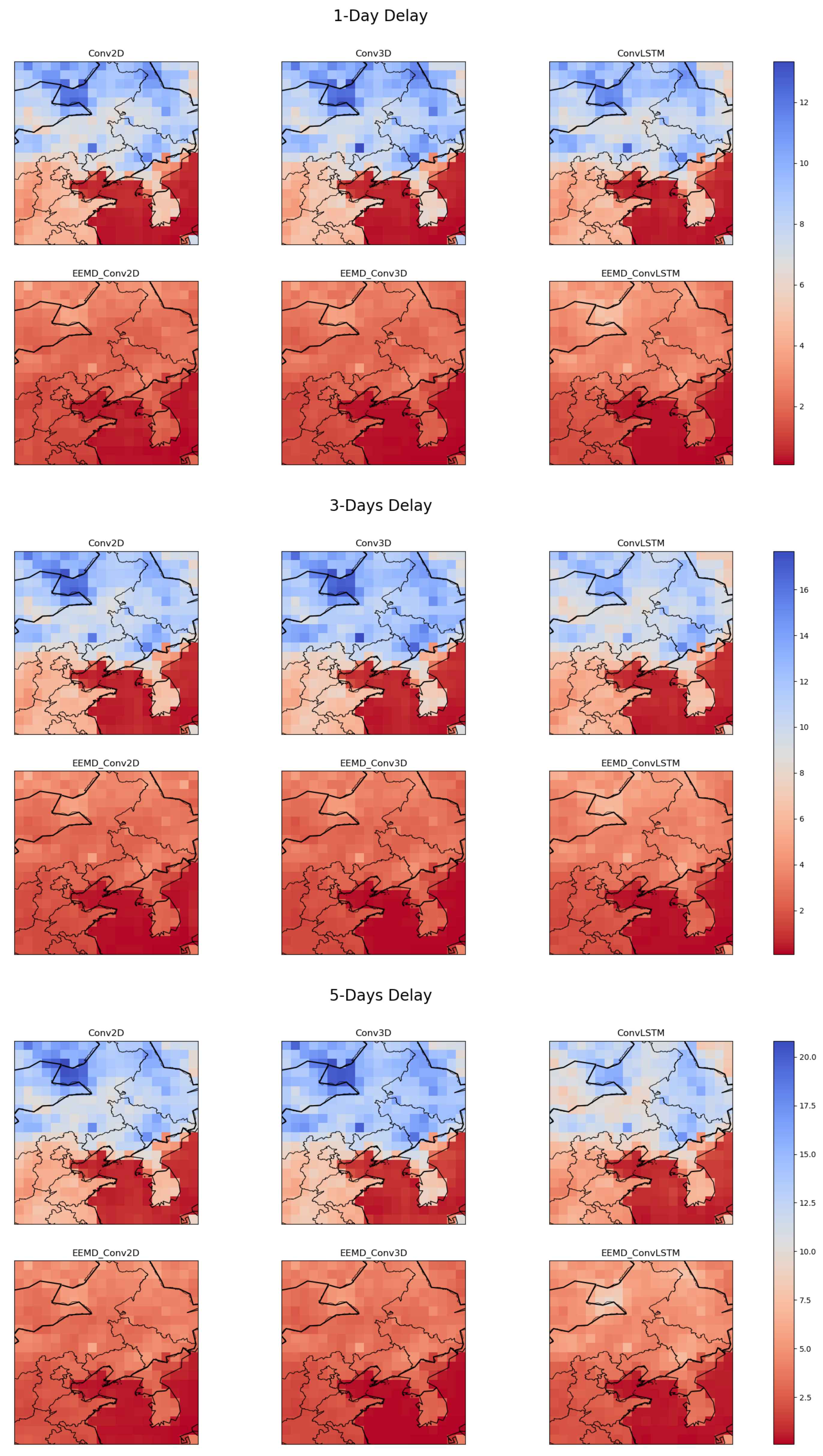
3.1. Results

After the models have been trained, we input the test data into each model and obtain the corresponding prediction results. The prediction results and the true values are simultaneously reshaped to a 1-dimensional series, and the performance of the models is assessed using the evaluation metrics. Performance of the models is shown in

Table 3. Estimation results for each model with different delays after training with the ERA5 dataset.

Delay	Models	MAE	MSE	RMSE	${\mathit{R}}^{\mathbf{2}}$	MAPE
1 Day	PF	1.4749	4.6189	2.1492	0.9713	29.87%
	Conv2D	1.7371	5.9179	2.4327	0.9626	40.65%
	Conv3D	1.7899	6.3363	2.5172	0.9598	42.36%
	ConvLSTM	1.7301	5.8763	2.4241	0.9634	40.33%
	EEMD-Conv2D	0.9952	1.775	1.3323	0.9887	16.22%
	EEMD-Conv3D	0.9656	1.7151	1.3096	0.9893	17.90%
	EEMD-ConvLSTM	1.0625	2.1374	1.462	0.9868	21.54%
3 Days	PF	2.2058	9.7061	3.1155	0.9392	53.00%
	Conv2D	2.0167	7.9812	2.8251	0.9489	44.86%
	Conv3D	2.1032	8.6639	2.9434	0.9442	46.91%
	ConvLSTM	1.9651	7.359	2.7128	0.9516	46.30%
	EEMD-Conv2D	1.1403	2.3792	1.5424	0.985	19.33%
	EEMD-Conv3D	1.0942	2.2378	1.4959	0.9858	19.31%
	EEMD-ConvLSTM	1.2281	2.8185	1.6789	0.9819	19.72%
5 Days	PF	2.4653	11.8385	3.4407	0.9252	59.90%
	Conv2D	2.1978	9.3635	3.06	0.9387	54.72%
	Conv3D	2.3094	10.2386	3.1998	0.9327	54.94%
	ConvLSTM	2.0861	8.2726	2.8762	0.949	65.03%
	EEMD-Conv2D	1.2865	3.002	1.7326	0.9807	27.41%
	EEMD-Conv3D	1.2056	2.7216	1.6497	0.9826	25.90%
	EEMD-ConvLSTM	1.3976	3.6842	1.9194	0.9768	21.39%

. When predicting ST with a one-day delay, DL models using raw data input did not work as well as PF. In contrast, when the DL models used the EEMD-processed data as input, the prediction performance was significantly improved. In addition to this, the DL model combined with EEMD performs better than PF’s performance. Under the same latency conditions, ConvLSTM has better performance than Conv2D and Conv3D in predicting ST using machine models without EEMD. In addition, when the model is combined with EEMD, EEMD-Conv3D has the best performance.

When the latency of the prediction increases, all models’ performance decreases. The most significant performance degradation among all models is PF, which already performs worse than the other DL models. In addition, among the DL models, the models that incorporate EEMD all perform better. Even the performance under 5-day delay outperformed the DL models without EEMD under 1-day delay. Figure 4 is scatter plots of the predicted and true values, which shows the degree of fit between the predicted and observed values of the DL model. As seen in the scatter plot, the DL model incorporating EEMD has a better fit. As the delay increases, the predicted values of the model with EEMD still fit well. With the help of EEMD, models are better able to overcome the decrease in accuracy of the prediction due to the increase in latency.

For three different delay cases, we randomly select the observation of a particular day to compare with the predicted results of each model. Figure 5 shows the spatial pattern of ST on a random day. The EEMD-based models have a high spatial similarity to the observations. The $R^2$ heat map and MSE heat map based on the observed and predicted values are shown in Figure 6 and Figure 7. It can be seen that the overall fit of the predicted values of each model decreases as the delay increases. However, for a particular delay, the model with EEMD has a better fit. Among the models combined with EEMD, the predicted values of EEMD-Conv3D have the best fit to the observed values.

3.2. Discussion

ST is an important variable in the field of meteorology and is closely linked to seed germination, plant growth, plant root activity, etc. [38]. It also affects the decomposition of organic matter in the soil and the release of carbon dioxide [39]. In order to accurately predict ST, deep learning models using ANN and LSTM have been proposed. These models provide useful insights on solving this problem and have been shown to have better performance than statistical models in predicting ST [15]. However, these prediction models for the time series of ST in a particular area or site are not applicable to the prediction of spatiotemporal ST. To ensure the spatial correlation of spatiotemporal ST, it is necessary to use models with convolution operators such as CNN [40]. It is commonly used in problems such as image classification, computer vision, etc. CNN can be applied to spatiotemporal ST prediction because the convolution operator can better handle the spatial features of the data [24]. In addition, Shi et al. proposed ConvLSTM also solves the problem of data in spatial dimension [25].

As seen in the results, DL models have a role in predicting spatiotemporal ST. Although they did not perform as well as PF in short-term prediction, DL models outperformed PF as the prediction delay increased. Unlike the direct data comparison, DL models are able to capture certain information through the spatiotemporal relationship of the data and use it to guide the predictive ability of the model. Although the results are not ideal and flawed, DL models have a tendency to fit the predicted values to the observed values when compared to the PF that directly uses the observations from a few days ago as the predicted values. Among DL models, ConvLSTM has the best performance. In contrast, Conv3D, whose convolutional kernel can only slide in the temporal dimension, does not perform as well as Conv2D, whose convolutional kernel can only slide in the spatial dimension. According to the model structure, Conv2D has 10 consecutive days of ST on the channel, while Conv3D has only 1 day of ST. Convolutional kernels of Conv3D are not sized to cover the complete time period in the time dimension. So the amount of information in the time dimension could affect the prediction results. For ConvLSTM, although each LSTM cell only inputs the soil temperature tensor for one time slice, the structure of the RNN guarantees the information in the time dimension [36]. In addition, the special gate structure of LSTM cells not only solves the problem of long-term dependence, but also controls the amount of historical state information passed through the forgetting gate [7,25]. So the ConvLSTM performs better in the three models.

EEMD processing has played an important role in enhancing DL models. It has been successful in many time series prediction models to enhance the accuracy of prediction [27,41,42]. In our experiments, DL models with EEMD incorporation have a significant improvement in prediction accuracy and performance. EEMD decomposes the temperature series in the temporal dimension into IMFs and residual series. These IMFs can better reflect the local characteristics of the original data and can better describe the trend of ST, resulting in a significant improvement in the performance of all models. As IMFs bring elevation in the number of channels, the 3D convolutional kernel is able to obtain more partial information. The excessive number of channels in EEMD-Conv2D may lead to overfitting and make it less effective than EEMD-Conv3D. In addition, one convolution operator in EEMD-ConvLSTM cell is not enough to cope with the processing of more local features caused by the increase of channels. Therefore, EEMD-Conv3D is more suitable for the prediction of spatiotemporal data.

4. Conclusions

Predicting spatiotemporal ST one or more days in advance is challenging. Unlike when predicting the ST at a site, only a continuous sequence needs to be paid attention to. In predicting spatiotemporal ST, attention also needs to be paid to the spatial characteristics of the data. Therefore, we chose Conv2D and Conv3D, which can handle spatiotemporal properties, to predict ST. In addition to them, ConvLSTM, which uses convolutional computation to replace the fully connected weight computation in traditional LSTM, is also used to predict spatiotemporal ST. On the basis of these three DL models, we bring in a signal decomposition method EEMD. EEMD was used to decompose the ST sequence for each grid in the temporal dimension. The decomposed data maintains connections in the spatial dimension and extends features in the temporal dimension. After comparing the prediction performance with and without EEMD, the results show that the prediction performance of the models with EEMD are significantly improved. Among all models, EEMD-Conv3D has the best performance in predicting spatiotemporal ST. In this paper, we evaluate our models on the ST prediction problem, but it is not limited to this domain. We expect the results of this article to be useful in handling more fields related to spatiotemporal data.

References

1. Lai, L.; Zhao, X.; Jiang, L.; Wang, Y.; Luo, L.; Zheng, Y.; Chen, X.; Rimmington, G.M. Soil respiration in different agricultural and natural ecosystems in an arid region. PLoS ONE 2012, 7, e48011. [Google Scholar] [CrossRef]
2. Liang, L.; Riveros-Iregui, D.; Emanuel, R.; McGlynn, B. A simple framework to estimate distributed soil temperature from discrete air temperature measurements in data-scarce regions. J. Geophys. Res. Atmos. 2014, 119, 407–417. [Google Scholar] [CrossRef]
3. Onwuka, B.; Mang, B. Effects of soil temperature on some soil properties and plant growth. Adv. Plants Agric. Res 2018, 8, 34–37. [Google Scholar] [CrossRef]
4. Zhang, Y.; Chen, W.; Smith, S.L.; Riseborough, D.W.; Cihlar, J. Soil temperature in Canada during the twentieth century: Complex responses to atmospheric climate change. J. Geophys. Res. D Atmos. 2005, 110, 1–15. [Google Scholar] [CrossRef]
5. Harvey, A.C.; Todd, P. Forecasting economic time series with structural and Box-Jenkins models: A case study. J. Bus. Econ. Stat. 1983, 1, 299–307. [Google Scholar] [CrossRef]
6. Specht, D.F. A general regression neural network. IEEE Trans. Neural Netw. 1991, 2, 568–576. [Google Scholar] [CrossRef] [PubMed] [Green Version]
7. Hochreiter, S.; Schmidhuber, J. Long short-term memory. Neural Comput. 1997, 9, 1735–1780. [Google Scholar] [CrossRef]
8. Dorffner, G. Neural networks for time series processing. Neural Netw. World 1996, 6, 447–468. [Google Scholar]
9. Granger, C.; Andersen, A. Non-linear time series modelling. In Applied Time Series Analysis I; Findley, D.F., Ed.; Academic Press: Cambridge, MA, USA, 1978; pp. 25–38. [Google Scholar] [CrossRef]
10. Shirvani, A.; Moradi, F.; Moosavi, A.A. Time series modelling of increased soil temperature anomalies during long period. Int. Agrophysics 2015, 29, 509–515. [Google Scholar] [CrossRef] [Green Version]
11. Chen, J.F.; Wang, W.M.; Huang, C.M. Analysis of an adaptive time-series autoregressive moving-average (ARMA) model for short-term load forecasting. Electr. Power Syst. Res. 1995, 34, 187–196. [Google Scholar] [CrossRef]
12. Mihalakakou, G. On estimating soil surface temperature profiles. Energy Build. 2002, 34, 251–259. [Google Scholar] [CrossRef]
13. Lekkas, D.; Onof, C.; Lee, M.; Baltas, E. Application of artificial neural networks for flood forecasting. Glob. Nest 2004, 6, 205–211. [Google Scholar] [CrossRef]
14. Abdel-Aal, R.E. Hourly temperature forecasting using abductive networks. Eng. Appl. Artif. Intell. 2004, 17, 543–556. [Google Scholar] [CrossRef]
15. Bilgili, M. Prediction of soil temperature using regression and artificial neural network models. Meteorol. Atmos. Phys. 2010, 110, 59–70. [Google Scholar] [CrossRef]
16. Tabari, H.; Hosseinzadeh Talaee, P.; Willems, P. Short-term forecasting of soil temperature using artificial neural network. Meteorol. Appl. 2015, 22, 576–585. [Google Scholar] [CrossRef] [Green Version]
17. Salcedo-Sanz, S.; Deo, R.; Carro-Calvo, L.; Saavedra-Moreno, B. Monthly prediction of air temperature in Australia and New Zealand with machine learning algorithms. Theor. Appl. Climatol. 2016, 125, 13–25. [Google Scholar] [CrossRef]
18. Kisi, O.; Sanikhani, H.; Cobaner, M. Soil temperature modeling at different depths using neuro-fuzzy, neural network, and genetic programming techniques. Theor. Appl. Climatol. 2017, 129, 833–848. [Google Scholar] [CrossRef]
19. Delbari, M.; Sharifazari, S.; Mohammadi, E. Modeling daily soil temperature over diverse climate conditions in Iran—A comparison of multiple linear regression and support vector regression techniques. Theor. Appl. Climatol. 2019, 135, 991–1001. [Google Scholar] [CrossRef]
20. Tokgöz, A.; Ünal, G. A RNN based time series approach for forecasting turkish electricity load. In Proceedings of the 2018 26th Signal Processing and Communications Applications Conference (SIU), Izmir, Turkey, 2–5 May 2018; pp. 1–4. [Google Scholar] [CrossRef]
21. Hewage, P.; Behera, A.; Trovati, M.; Pereira, E. Long-Short Term Memory for an Effective Short-Term Weather Forecasting Model Using Surface Weather Data. In IFIP Advances in Information and Communication Technology; Springer: Berlin/Heidelberg, Germany, 2019; Volume 559, pp. 382–390. [Google Scholar] [CrossRef] [Green Version]
22. Lawrence, S.; Giles, C.L.; Tsoi, A.C.; Back, A.D. Face recognition: A convolutional neural-network approach. IEEE Trans. Neural Netw. 1997, 8, 98–113. [Google Scholar] [CrossRef] [Green Version]
23. Ji, S.; Xu, W.; Yang, M.; Yu, K. 3D convolutional neural networks for human action recognition. IEEE Trans. Pattern Anal. Mach. Intell. 2012, 35, 221–231. [Google Scholar] [CrossRef] [PubMed] [Green Version]
24. Tran, D.; Bourdev, L.; Fergus, R.; Torresani, L.; Paluri, M. Learning spatiotemporal features with 3D convolutional networks. In Proceedings of the IEEE International Conference on Computer Vision (ICCV), Santiago, Chile, 7–13 December 2015; Volume 2015, pp. 4489–4497. [Google Scholar] [CrossRef] [Green Version]
25. Shi, X.; Chen, Z.; Wang, H.; Yeung, D.Y.; Wong, W.K.; Woo, W.C. Convolutional LSTM network: A machine learning approach for precipitation nowcasting. Adv. Neural Inf. Process. Syst. 2015, 2015, 802–810. [Google Scholar]
26. Wu, Z.; Huang, N.E. Ensemble empirical mode decomposition: A noise-assisted data analysis method. Adv. Adapt. Data Anal. 2009, 1, 1–41. [Google Scholar] [CrossRef]
27. Wang, W.c.; Chau, K.w.; Xu, D.m.; Chen, X.Y. Improving forecasting accuracy of annual runoff time series using ARIMA based on EEMD decomposition. Water Resour. Manag. 2015, 29, 2655–2675. [Google Scholar] [CrossRef]
28. Zhang, N.; Lin, A.; Shang, P. Multidimensional k-nearest neighbor model based on EEMD for financial time series forecasting. Phys. A Stat. Mech. Its Appl. 2017, 477, 161–173. [Google Scholar] [CrossRef]
29. Zhang, X.; Zhang, Q.; Zhang, G.; Nie, Z.; Gui, Z.; Que, H. A novel hybrid data-driven model for daily land surface temperature forecasting using long short-term memory neural network based on ensemble empirical mode decomposition. Int. J. Environ. Res. Public Health 2018, 15, 1032. [Google Scholar] [CrossRef] [Green Version]
30. Huang, N.E.; Shen, Z.; Long, S.R. A new view of nonlinear water waves: The Hilbert spectrum. Annu. Rev. Fluid Mech. 1999, 31, 417–457. [Google Scholar] [CrossRef] [Green Version]
31. Huang, N.E.; Shen, Z.; Long, S.R.; Wu, M.C.; Shih, H.H.; Zheng, Q.; Yen, N.C.; Tung, C.C.; Liu, H.H. The empirical mode decomposition and the Hilbert spectrum for nonlinear and non-stationary time series analysis. Proc. R. Soc. Lond. Ser. A Math. Phys. Eng. Sci. 1998, 454, 903–995. [Google Scholar] [CrossRef]
32. Kalchbrenner, N.; Grefenstette, E.; Blunsom, P. A convolutional neural network for modelling sentences. In Proceedings of the 52nd Annual Meeting of the Association for Computational Linguistics, Baltimore, MD, USA, 22–27 June 2014; Volume 1, pp. 655–665. [Google Scholar] [CrossRef] [Green Version]
33. Krizhevsky, A.; Sutskever, I.; Hinton, G.E. Imagenet classification with deep convolutional neural networks. Adv. Neural Inf. Process. Syst. 2012, 25, 1097–1105. [Google Scholar] [CrossRef]
34. Xu, L.; Ren, J.S.; Liu, C.; Jia, J. Deep convolutional neural network for image deconvolution. Adv. Neural Inf. Process. Syst. 2014, 2, 1790–1798. [Google Scholar]
35. Tran, D.; Wang, H.; Torresani, L.; Ray, J.; Lecun, Y.; Paluri, M. A Closer Look at Spatiotemporal Convolutions for Action Recognition. In Proceedings of the IEEE Conference on Computer Vision and Pattern Recognition (CVPR), Salt Lake City, UT, USA, 18–23 June 2018; pp. 6450–6459. [Google Scholar]
36. Zaremba, W.; Sutskever, I.; Vinyals, O. Recurrent Neural Network Regularization. arXiv 2014, arXiv:1409.2329. [Google Scholar]
37. Rasp, S.; Dueben, P.D.; Scher, S.; Weyn, J.A.; Mouatadid, S.; Thuerey, N. WeatherBench: A Benchmark Data Set for Data-Driven Weather Forecasting. J. Adv. Model. Earth Syst. 2020, 12, e2020MS002203. [Google Scholar] [CrossRef]
38. Tenge, A.J.; Kaihura, F.B.; Lal, R.; Singh, B.R. Diurnal soil temperature fluctuations for different erosion classes of an oxisol at Mlingano, Tanzania. Soil Tillage Res. 1998, 49, 211–217. [Google Scholar] [CrossRef]
39. Paul, K.I.; Polglase, P.J.; Smethurst, P.J.; O’Connell, A.M.; Carlyle, C.J.; Khanna, P.K. Soil temperature under forests: A simple model for predicting soil temperature under a range of forest types. Agric. For. Meteorol. 2004, 121, 167–182. [Google Scholar] [CrossRef]
40. Shomron, G.; Weiser, U. Spatial correlation and value prediction in convolutional neural networks. IEEE Comput. Archit. Lett. 2019, 18, 10–13. [Google Scholar] [CrossRef] [Green Version]
41. Wu, Y.X.; Wu, Q.B.; Zhu, J.Q. Improved EEMD-based crude oil price forecasting using LSTM networks. Phys. A: Stat. Mech. Its Appl. 2019, 516, 114–124. [Google Scholar] [CrossRef]
42. Tan, Q.F.; Lei, X.H.; Wang, X.; Wang, H.; Wen, X.; Ji, Y.; Kang, A.Q. An adaptive middle and long-term runoff forecast model using EEMD-ANN hybrid approach. J. Hydrol. 2018, 567, 767–780. [Google Scholar] [CrossRef]
Figure 1. The geographic extent of the experimental area on the map (33° N–52° N, 112° E–131° E).
Sustainability 13 09174 g001
Figure 2. The process of two kinds of convolution kernels in convolution operation.
Sustainability 13 09174 g002
Figure 3. Process of model training and overall framework of the experiment.
Sustainability 13 09174 g003
Figure 4. Scatter plots of predicted and observed ST values for each model at different delays.
Sustainability 13 09174 g004
Figure 5. Spatial model of ST observed values and predicted values of each model on a random day.
Sustainability 13 09174 g005
Figure 6. Heat map of R 2 , each grid represents the R 2 calculated from the observed and predicted values of this grid (Larger R 2 represents a better fit).
Sustainability 13 09174 g006
Figure 7. Heat map of MSE, each grid represents the MSE calculated from the observed and predicted values of this grid (Smaller MSE represents a better fit).
Sustainability 13 09174 g007