
Carbon Productivity and Mitigation: Evidence from Industrial Development and Urbanization in the Central and Western Regions of China


Abstract
:1. Introduction
2. Literature Review
3. Methods and Data
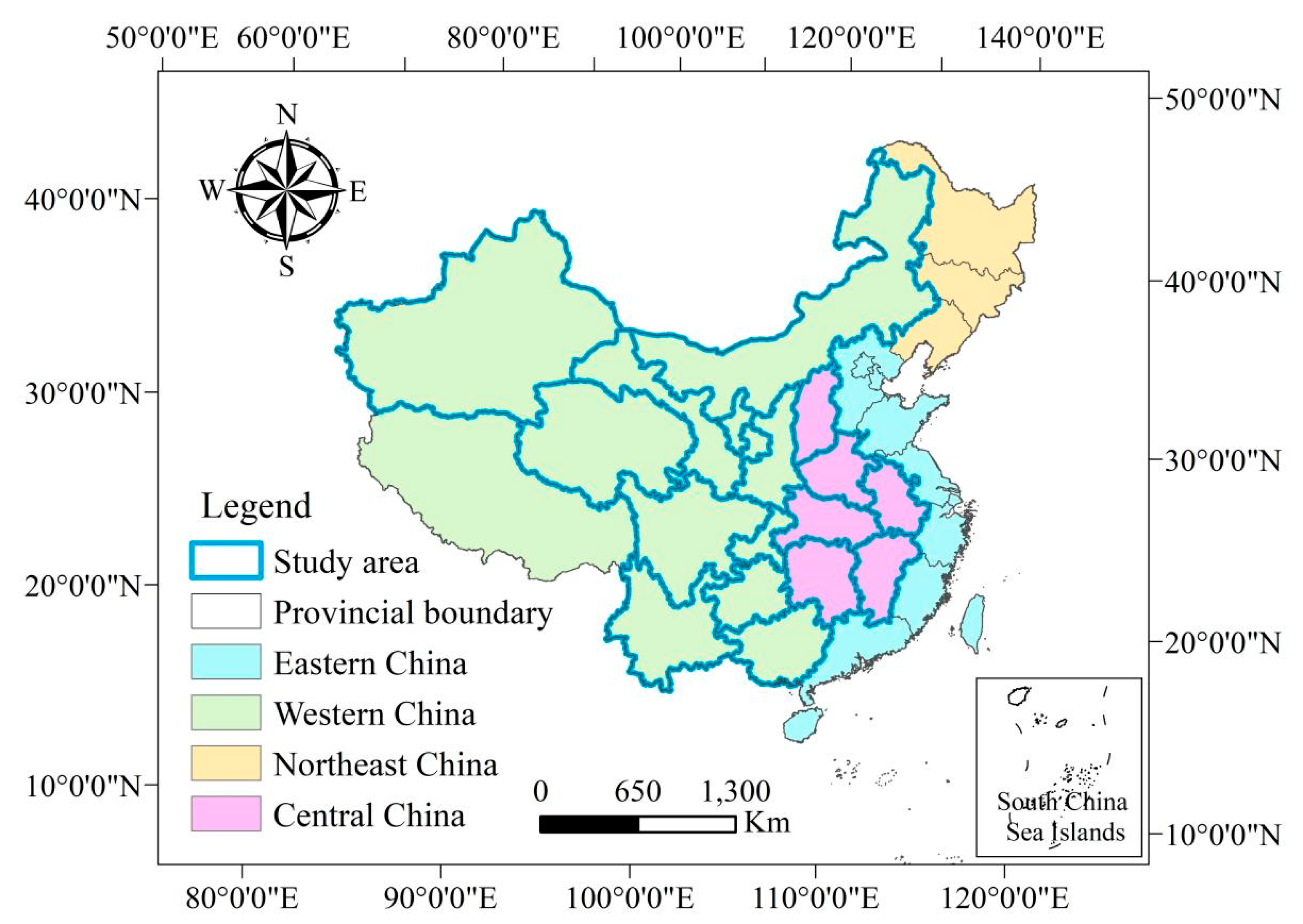
3.1. Study Area
3.2. Variables
3.2.1. Carbon Productivity (CP)
3.2.2. Industrial Development Level: TL, TK, TS
3.2.3. Urbanization Level
3.2.4. Data Sources and Processing
3.3. Model Description
3.3.1. Spatial Weight Matrix Calculation
3.3.2. Spatial Autocorrelation Model
3.3.3. Spatial Econometric Model
4. Results and Analysis
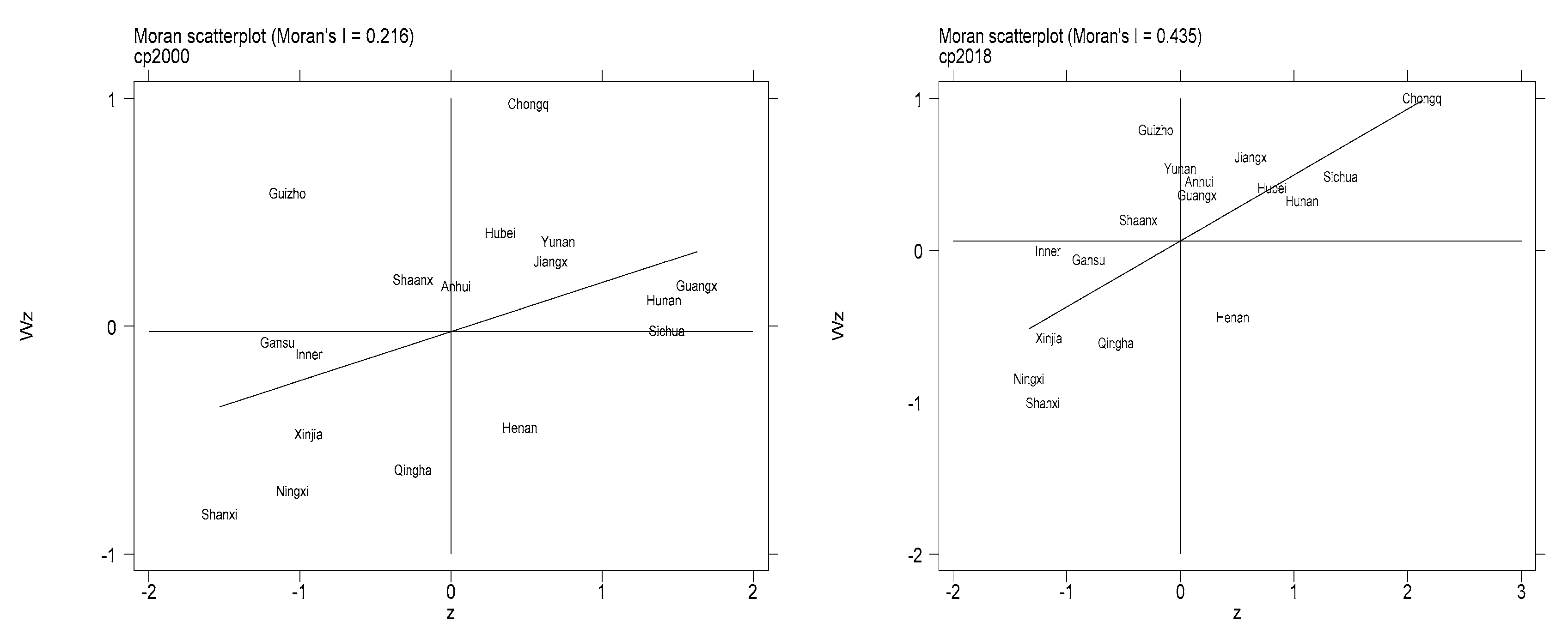
4.1. Spatial Autocorrelation Test
4.2. Spatial Model Results
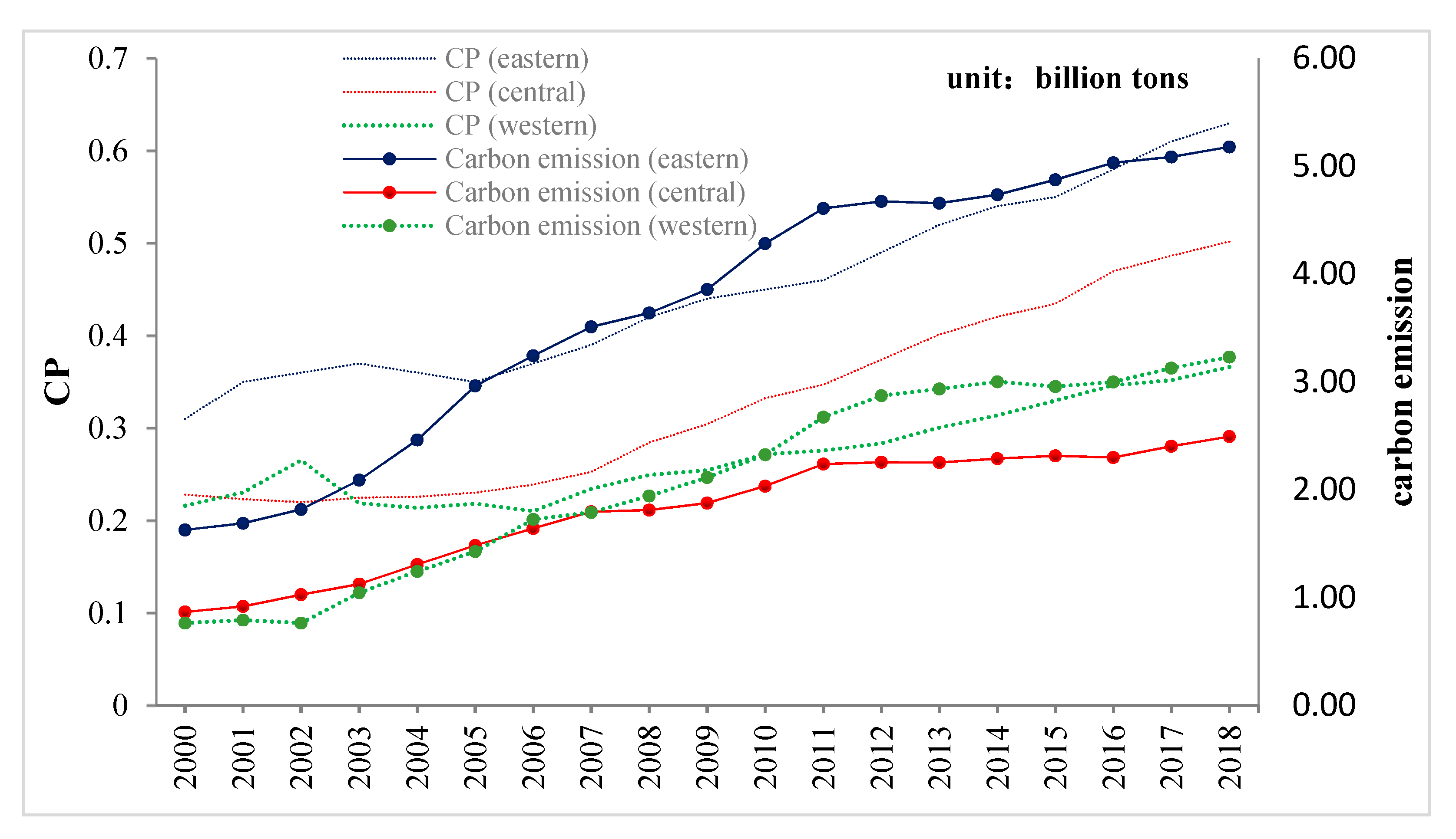
4.3. Carbon Productivity (CP)
4.4. Industrial Development and Its Impacts on CP
4.4.1. Workforce Allocation (TL)
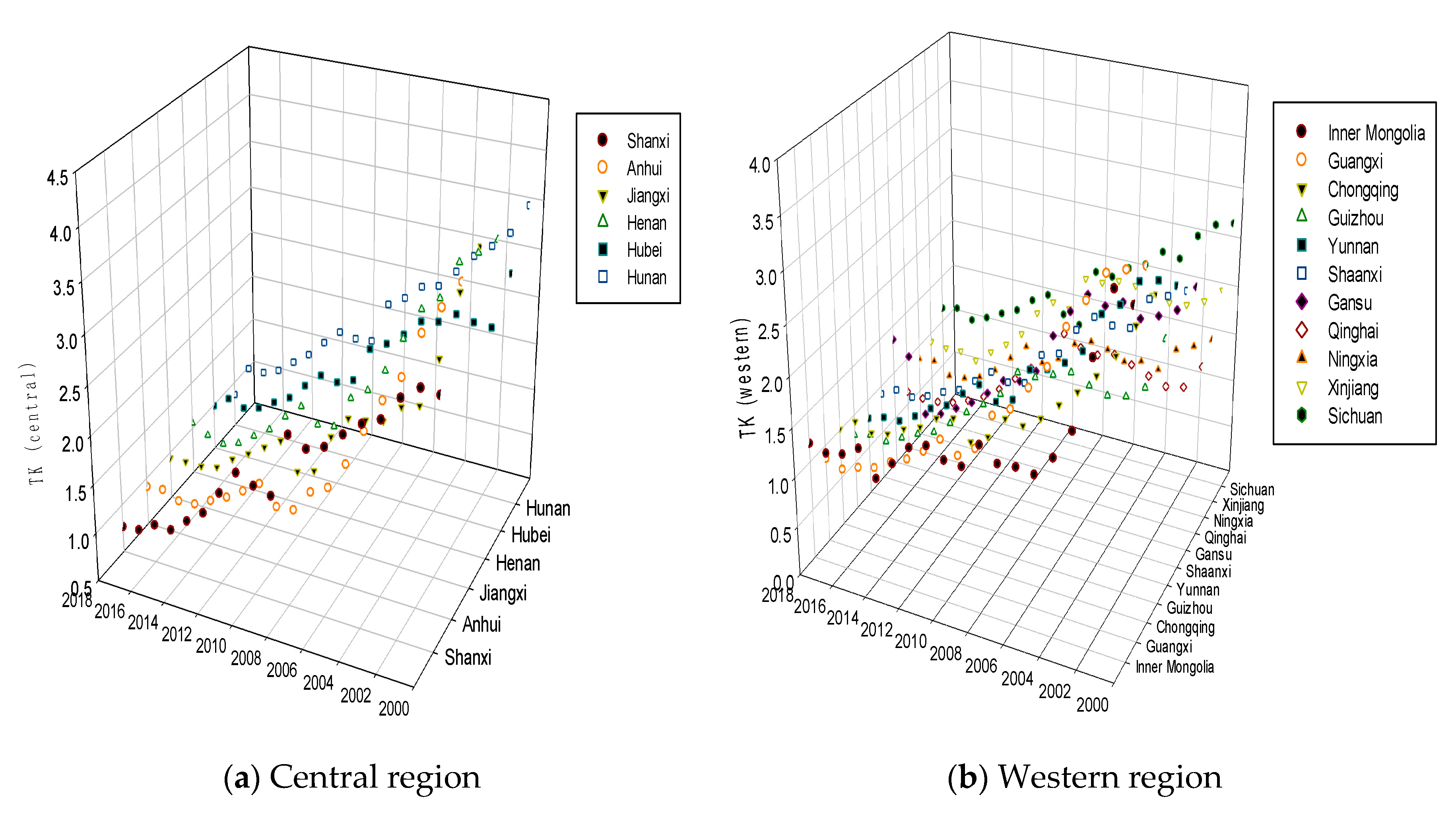
4.4.2. Economic Output Efficiency of Fixed Investments (TK)
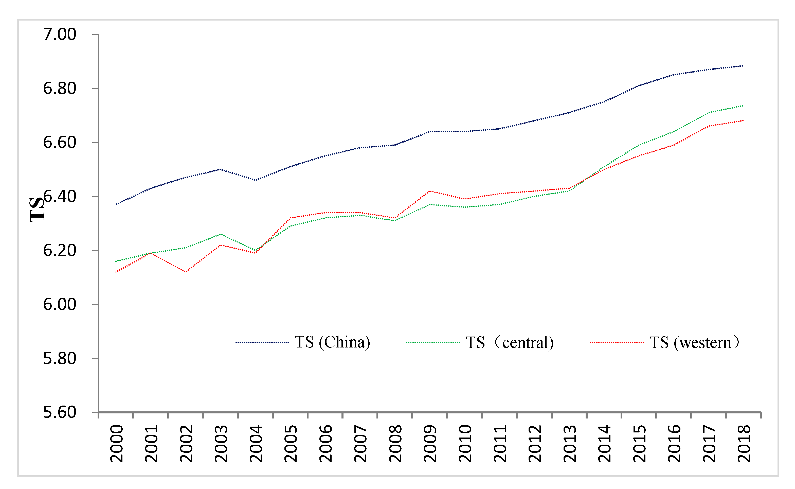
4.4.3. Industrial Structure Upgrading (TS)
4.5. Urbanization Level and Its Impacts on CP
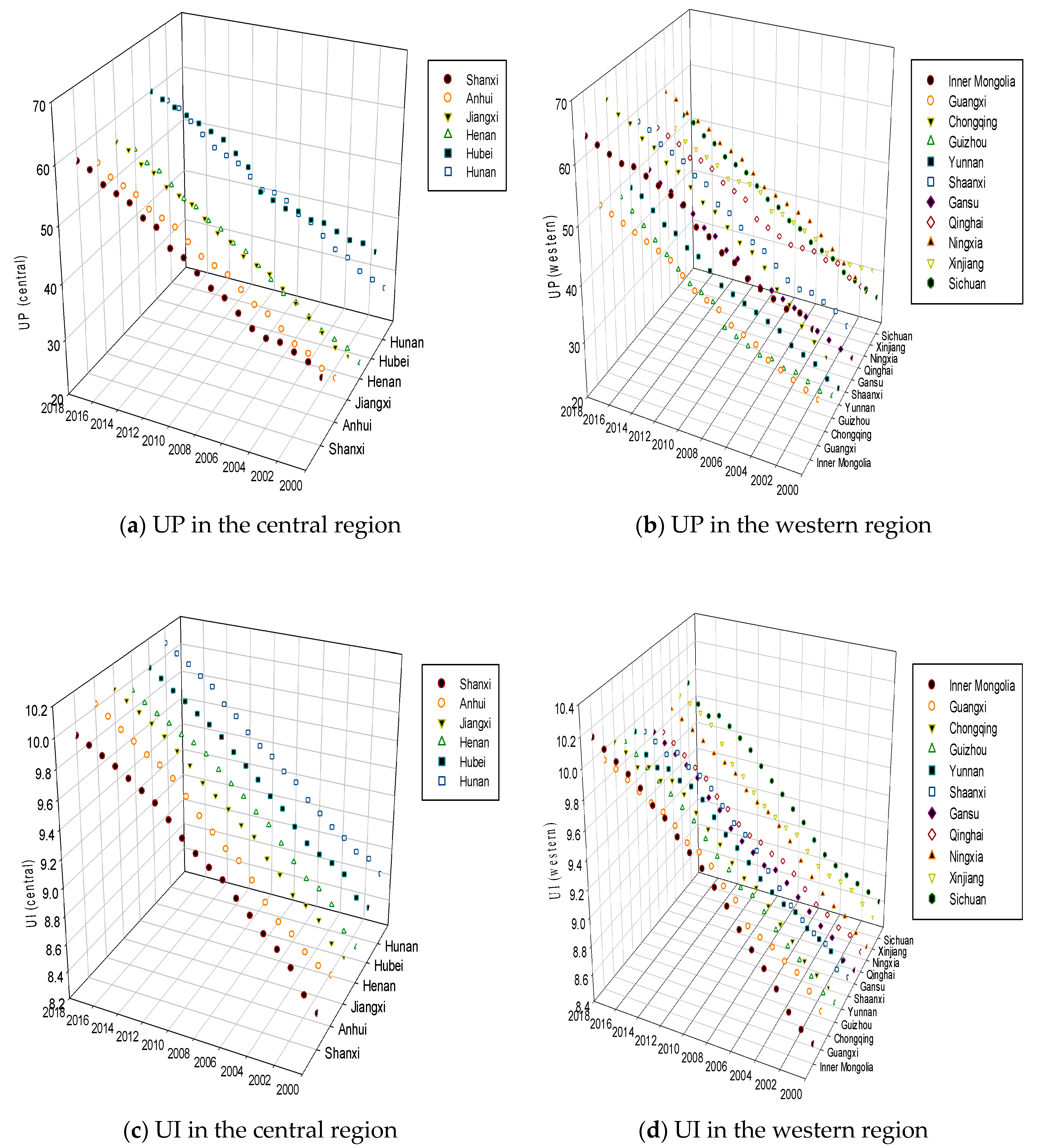
4.5.1. Population Urbanization (UP)
4.5.2. Urban Resident Disposable Income (UI)
5. Discussion
5.1. TL, TK, TS, and CP
5.2. UI, UP, and CP
6. Conclusions and Policy Suggestions
Author Contributions
Funding
Institutional Review Board Statement
Informed Consent Statement
Data Availability Statement
Acknowledgments
Conflicts of Interest
References
- U.S. Energy Information Administration (EIA). International Energy Outlook 2019 with Projections to 2050; Energy Information Administration: Washington, DC, USA, 2019.
- Dong, K.; Dong, X.; Jiang, Q. How renewable energy consumption lower global CO2 emissions? Evidence from countries with different income levels. World Econ. 2020, 43, 1665–1698. [Google Scholar] [CrossRef]
- Zhao, J.; Jiang, Q.; Dong, X.; Dong, K. Assessing energy poverty and its effect on CO2 emissions: The case of China. Energy Econ. 2021, 97, 105191. [Google Scholar] [CrossRef]
- Khan, Z.; Murshed, M.; Dong, K.; Yang, S. The roles of export diversification and composite country risks in carbon emissions abatement: Evidence from the signatories of the regional comprehensive economic partnership agreement. Appl. Econ. 2021, 53, 4769–4787. [Google Scholar] [CrossRef]
- Wang, X.; Tang, X.; Zhang, B.; McLellan, B.C.; Lv, Y. Provincial Carbon Emissions Reduction Allocation Plan in China Based on Consumption Perspective. Sustainabity 2018, 10, 1342. [Google Scholar] [CrossRef] [Green Version]
- Kaya, Y.; Yokobori, K. Environment, Energy and Economy: Strategies for Sustainability; Bookwell Publications: New Delhi, India, 1999. [Google Scholar]
- Report, M. The Carbon Productivity Challenge: Curbing Climate Change and Sustaining Economic Growth; Mckinsey Global Institute: Sydney, Australia, 2008. [Google Scholar]
- Yu, S.; Zheng, S.; Li, X.; Li, L. China can peak its energy-related carbon emissions before 2025: Evidence from industry restructuring. Energy Econ. 2018, 73, 91–107. [Google Scholar] [CrossRef]
- Wang, W.; Li, M.; Zhang, M. Study on the changes of the decoupling indicator between energy-related CO2 emission and GDP in China. Energy 2017, 128, 11–18. [Google Scholar] [CrossRef]
- Luan, B.; Zou, H.; Chen, S.; Huang, J. The effect of industrial structure adjustment on China’s energy intensity: Evidence from linear and nonlinear analysis. Energy 2021, 218, 119517. [Google Scholar] [CrossRef]
- Zhang, L.; Zhou, P. A non-compensatory composite indicator approach to assessing low-carbon performance. Eur. J. Oper. Res. 2018, 270, 352–361. [Google Scholar] [CrossRef]
- Lin, B.; Du, K. Energy and CO2 emissions performance in China’s regional economies: Do market-oriented reforms matter? Energy Policy 2015, 78, 113–124. [Google Scholar] [CrossRef] [Green Version]
- Liu, B.; Tian, C.; Li, Y.; Song, H.; Ma, Z. Research on the effects of urbanization on carbon emissions efficiency of urban agglomerations in China. J. Clean. Prod. 2018, 197, 1374–1381. [Google Scholar] [CrossRef]
- Li, W.; Wang, L. The First “Sketch” of Urban Energy Development in China (Translated from Mandarin). China Energy News, 22 October 2018. [Google Scholar]
- Chen, M.; Gong, Y.; Lu, D.; Ye, C. Build a people-oriented urbanization: China’s new-type urbanization dream and Anhui model. Land Use Policy 2019, 80, 1–9. [Google Scholar] [CrossRef]
- Anselin, L. Spatial Effects in Econometric Practice in Environmental and Resource Economics. Am. J. Agric. Econ. 2001, 83, 705–710. [Google Scholar] [CrossRef]
- Tian, K.; Dietzenbacher, E.; Yan, B.; Duan, Y. Upgrading or downgrading: China’s regional carbon emission intensity evolution and its determinants. Energy Econ. 2020, 91, 104891. [Google Scholar] [CrossRef]
- Zheng, X.; Wang, R.; Du, Q. How does industrial restructuring influence carbon emissions: City-level evidence from China. J. Environ. Manag. 2020, 276, 111093. [Google Scholar] [CrossRef]
- Wang, G.; Deng, X.; Wang, J.; Zhang, F.; Liang, S. Carbon productivity in China: A spatial panel data analysis. China Econ. Rev. 2019, 56, 78–89. [Google Scholar] [CrossRef]
- Lan, F.; Sun, L.; Pu, W. Research on the influence of manufacturing agglomeration modes on regional carbon emission and spatial effect in China. Econ. Model. 2021, 96, 346–352. [Google Scholar] [CrossRef]
- Benjamin, N.I.; Lin, B. Quantile analysis of carbon emissions in China metallurgy industry. J. Clean. Prod. 2020, 243, 118534. [Google Scholar] [CrossRef]
- Adesina, A. Recent advances in the concrete industry to reduce its carbon dioxide emissions. Environ. Chall. 2020, 1, 100004. [Google Scholar] [CrossRef]
- Cheng, Z.; Li, L.; Liu, J. Industrial structure, technical progress and carbon intensity in China’s provinces. Renew. Sustain. Energy Rev. 2018, 81, 2935–2946. [Google Scholar] [CrossRef]
- Zhu, B.; Zhang, T. The impact of cross-region industrial structure optimization on economy, carbon emissions and energy consumption: A case of the Yangtze River Delta. Sci. Total. Environ. 2021, 778, 146089. [Google Scholar] [CrossRef]
- Ullah, S.; Ozturk, I.; Usman, A.; Majeed, M.T.; Akhtar, P. On the asymmetric effects of premature deindustrialization on CO2 emissions: Evidence from Pakistan. Environ. Sci. Pollut. Res. 2020, 27, 13692–13702. [Google Scholar] [CrossRef]
- Muhammad, S.; Long, X.; Salman, M.; Dauda, L. Effect of urbanization and international trade on CO2 emissions across 65 belt and road initiative countries. Energy 2020, 196, 117102. [Google Scholar] [CrossRef]
- Li, S.; Wang, S. Examining the effects of socioeconomic development on China’s carbon productivity: A panel data analysis. Sci. Total Environ. 2019, 659, 681–690. [Google Scholar] [CrossRef] [PubMed]
- Sun, W.; Huang, C. How does urbanization affect carbon emission efficiency? Evidence from China. J. Clean. Prod. 2020, 272, 122828. [Google Scholar] [CrossRef]
- Zhou, C.; Wang, S.; Wang, J. Examining the influences of urbanization on carbon dioxide emissions in the Yangtze River Delta, China: Kuznets curve relationship. Sci. Total. Environ. 2019, 675, 472–482. [Google Scholar] [CrossRef] [PubMed]
- Martínez-Zarzoso, I.; Maruotti, A. The effect of urbanization on CO2 emissions: Evidence from developing countries. Ecol. Econ. 2011, 70, 1344–1353. [Google Scholar] [CrossRef] [Green Version]
- Wang, W.-Z.; Liu, L.-C.; Liao, H.; Wei, Y.-M. Impacts of urbanization on carbon emissions: An empirical analysis from OECD countries. Energy Policy 2021, 151, 112171. [Google Scholar] [CrossRef]
- Chen, S.; Li, N.; Guan, J. Research on statistical methodology to investigate energy consumption in public buildings sector in China. Energy Convers. Manag. 2008, 49, 2152–2159. [Google Scholar] [CrossRef]
- Liobikiene, G.; Butkus, M. Scale, composition, and technique effects through which the economic growth, foreign direct investment, urbanization, and trade affect greenhouse gas emissions. Renew. Energy 2019, 132, 1310–1322. [Google Scholar] [CrossRef]
- Cai, B.; Guo, H.; Ma, Z.; Wang, Z.; Dhakal, S.; Cao, L. Benchmarking carbon emissions efficiency in Chinese cities: A comparative study based on high-resolution gridded data. Appl. Energy 2019, 242, 994–1009. [Google Scholar] [CrossRef]
- Wang, K.; Wu, M.; Sun, Y.; Shi, X.; Sun, A.; Zhang, P. Resource abundance, industrial structure, and regional carbon emissions efficiency in China. Resour. Policy 2019, 60, 203–214. [Google Scholar] [CrossRef]
- Zheng, H.; Gao, X.; Sun, Q.; Han, X.; Wang, Z. The impact of regional industrial structure differences on carbon emission differences in China: An evolutionary perspective. J. Clean. Prod. 2020, 257, 120506. [Google Scholar] [CrossRef]
- Sadorsky, P. The effect of urbanization on CO2 emissions in emerging economies. Energy Econ. 2014, 41, 147–153. [Google Scholar] [CrossRef]
- Liu, J.; Hou, X.; Wang, Z.; Shen, Y. Study the effect of industrial structure optimization on urban land-use efficiency in China. Land Use Policy 2021, 105, 105390. [Google Scholar] [CrossRef]
- Varian, H.R. Intermediate Microeconomics: A Modern Approach; W.W. Norton & Company: New York, NY, USA, 1999. [Google Scholar]
- Zhou, X.; Zhang, J.; Li, J. Industrial structural transformation and carbon dioxide emissions in China. Energy Policy 2013, 57, 43–51. [Google Scholar] [CrossRef]
- Moore, J.H. A Measure of Structural Change in Output. Rev. Income Wealth 1978, 24, 105–118. [Google Scholar] [CrossRef]
- Poumanyvong, P.; Kaneko, S. Does urbanization lead to less energy use and lower CO2 emissions? A cross-country analysis. Ecol. Econ. 2010, 70, 434–444. [Google Scholar] [CrossRef]
- Yang, G.; Wu, Q.; Tu, Y. Researchs of China’s regional carbon emission spatial correlation and its determinants:based on the method of social network analysis. J. Bus. Econ. 2016, 4, 56–68. [Google Scholar]
- Anselin, L. Spatial Econometrics: Methods and Models; Springer: Amsterdam, The Netherlands, 1988. [Google Scholar]
- LeSage, J.; Pace, K.R. Introduction to Spatial Econometrics; Chapman and Hall/CRC: London, UK, 2009. [Google Scholar]
- Liu, Y.; Wang, M.; Feng, C. Inequalities of China’s regional low-carbon development. J. Environ. Manag. 2020, 274, 111042. [Google Scholar] [CrossRef] [PubMed]
- Zhang, S.; Kharrazi, A.; Yu, Y.; Ren, H.; Hong, L.; Ma, T. What causes spatial carbon inequality? Evidence from China’s Yangtze River economic Belt. Ecol. Indic. 2021, 121, 107129. [Google Scholar] [CrossRef]
- Wu, Y.; Dong, S.; Huang, H.; Zhai, J.; Li, Y.; Huang, D. Quantifying urban land expansion dynamics through improved land management institution model: Application in Ningxia-Inner Mongolia, China. Land Use Policy 2018, 78, 386–396. [Google Scholar] [CrossRef]
- Li, L.; Qi, P. The impact of China’s investment increase in fixed assets on ecological environment: An empirical analysis. Energy Procedia 2011, 5, 501–507. [Google Scholar] [CrossRef] [Green Version]
- Zhang, W.; Feng, P. Differentiation research of CO2 emissions from energy consumption and their influencing mechanism on the industrial enterprises above designated size in Chinese industrial cities: Based on geographical detector method. Nat. Hazards 2020, 102, 645–658. [Google Scholar] [CrossRef] [Green Version]


| Fossil Fuel | Default Carbon Content (kgC/GJ) | Default Carbon Oxidation Rate | Calorific Value (KJ/kg, m3) | Carbon Emission Factor (kgC/kg, m3) |
|---|---|---|---|---|
| Raw coal | 25.8 | 1 | 20,908 | 0.53943 |
| Coke | 29.2 | 1 | 28,435 | 0.8303 |
| Crude oil | 20 | 1 | 41,816 | 0.83632 |
| Gasoline | 18.9 | 1 | 43,070 | 0.81402 |
| Kerosene | 19.6 | 1 | 43,070 | 0.84417 |
| Diesel | 20.2 | 1 | 42,652 | 0.86157 |
| Liquefied Petroleum gas | 21.2 | 1 | 41,816 | 0.88232 |
| Natural gas | 15.3 | 1 | 38,931 | 0.59564 |
| Variable | Obs | Mean | SD | Min | Max |
|---|---|---|---|---|---|
| CP (carbon productivity) | 323 | 0.32 | 0.19 | 0.07 | 1.13 |
| TL (workforce allocation) | 323 | 0.32 | 0.14 | 0.08 | 0.78 |
| TK (economic output efficiency of fixed investments) | 323 | 1.71 | 0.73 | 0.61 | 3.88 |
| TS (industrial structure upgrading) | 323 | 6.39 | 0.21 | 5.88 | 7.00 |
| UI (economic urbanization) | 323 | 9.30 | 0.43 | 8.46 | 10.14 |
| UP (population urbanization) | 323 | 0.42 | 0.10 | 0.23 | 0.66 |
| Time | Carbon Productivity | Time | Carbon Productivity | ||
|---|---|---|---|---|---|
| Moran’s I | p-Value | Moran’s I | p-Value | ||
| 2000 | 0.216 | 0.034 | 2009 | 0.277 | 0.010 |
| 2001 | 0.212 | 0.036 | 2010 | 0.302 | 0.006 |
| 2002 | 0.209 | 0.038 | 2011 | 0.341 | 0.002 |
| 2003 | 0.196 | 0.048 | 2012 | 0.348 | 0.002 |
| 2004 | 0.249 | 0.017 | 2013 | 0.363 | 0.001 |
| 2005 | 0.277 | 0.010 | 2014 | 0.372 | 0.001 |
| 2006 | 0.291 | 0.007 | 2015 | 0.396 | 0.000 |
| 2007 | 0.257 | 0.015 | 2016 | 0.404 | 0.000 |
| 2008 | 0.281 | 0.009 | 2017 | 0.424 | 0.000 |
| 2018 | 0.435 | 0.000 | |||
| Parameter | SEM | Regional Fixed Effects Model | Time Fixed Effects Model | Regional and Time Fixed Effects Model |
|---|---|---|---|---|
| −0.139 *** | −0.107 *** | −0.529 *** | −0.153 *** | |
| (−3.61) | (−2.80) | (−9.98) | (−3.85) | |
| 0.175 *** | 0.096 ** | −0.0523 | 0.191 *** | |
| −4.13 | −2.4 | (−0.88) | −3.95 | |
| 0.007 * | 0.009 ** | 0.016 ** | 0.007 | |
| −2.12 | −2.12 | −1.83 | −1.6 | |
| −0.217 *** | −0.156 *** | −0.090 | −0.230 *** | |
| (−7.67) | (−5.84) | (−1.52) | (−6.74) | |
| (UP^2) | 0.125 *** | 0.104 *** | 0.019 | 0.138 *** |
| −9.4 | −8.6 | −0.89 | −9.28 | |
| −0.031 *** | −0.041 *** | 0.084 *** | −0.044 *** | |
| (−3.74) | (−5.69) | −5.61 | (−3.97) | |
| 0.513 *** | 0.683 *** | 0.566 *** | ||
| −9.31 | −13.06 | −9.35 | ||
| lamdba | 0.599 *** | |||
| −9.91 | ||||
| sigma2_e | 0.0000896 *** | 0.00009 *** | 0.0003601 *** | 0.0000868 *** |
| −12.41 | −12.56 | −12.28 | −12.27 | |
| R-squared | 0.6863 | 0.6827 | 0.5466 | 0.6739 |
| Log-likelihood | 1035.605 | 1038.277 | 806.7826 | 1044.576 |
| LMLAG | 31.9960 *** | |||
| R-LMLAG | 33.1927 *** | |||
| LMERROR | 13.9696 *** | |||
| R-LMERROR | 15.1664 *** | |||
| Hausman | 28.52 (0.0001) | |||
| Observations | 323 | 323 | 323 | 323 |
| Variable | Direct Effect | Indirect Effect | Total Effect |
|---|---|---|---|
| TL | −0.111 *** | −0.105 ** | −0.216 *** |
| (−2.72) | (−2.52) | (−2.72) | |
| TS | 0.099 ** | 0.094 ** | 0.194 ** |
| −2.44 | −2.17 | −2.37 | |
| TK | 0.010 * | 0.010 ** | 0.020 ** |
| −2.28 | −2.01 | −2.2 | |
| UP | −0.165 *** | −0.157 *** | −0.322 *** |
| (−5.95) | (−4.01 ) | (−5.45 ) | |
| UP^2 | 0.110 *** | 0.105 *** | 0.214 *** |
| −9.1 | −4.72 | −7.64 | |
| UI | −0.043 *** | −0.041 *** | −0.085 *** |
| (−5.68) | (−3.62) | (−7.64) |
Publisher’s Note: MDPI stays neutral with regard to jurisdictional claims in published maps and institutional affiliations. |
© 2021 by the authors. Licensee MDPI, Basel, Switzerland. This article is an open access article distributed under the terms and conditions of the Creative Commons Attribution (CC BY) license (https://creativecommons.org/licenses/by/4.0/).
Share and Cite
Wu, Y.; Zheng, H.; Li, Y.; Delang, C.O.; Qian, J. Carbon Productivity and Mitigation: Evidence from Industrial Development and Urbanization in the Central and Western Regions of China. Sustainability 2021, 13, 9014. https://doi.org/10.3390/su13169014
Wu Y, Zheng H, Li Y, Delang CO, Qian J. Carbon Productivity and Mitigation: Evidence from Industrial Development and Urbanization in the Central and Western Regions of China. Sustainability. 2021; 13(16):9014. https://doi.org/10.3390/su13169014
Chicago/Turabian StyleWu, Yongjiao, Huazhu Zheng, Yu Li, Claudio O. Delang, and Jiao Qian. 2021. "Carbon Productivity and Mitigation: Evidence from Industrial Development and Urbanization in the Central and Western Regions of China" Sustainability 13, no. 16: 9014. https://doi.org/10.3390/su13169014
APA StyleWu, Y., Zheng, H., Li, Y., Delang, C. O., & Qian, J. (2021). Carbon Productivity and Mitigation: Evidence from Industrial Development and Urbanization in the Central and Western Regions of China. Sustainability, 13(16), 9014. https://doi.org/10.3390/su13169014