Abstract
One of the strategies of the European Green Deal is the increment of renewable integration in the civil sector and the mitigation of the impact of climate change. With a statistical and critical approach, the paper analyzes these aspects by means of a case study simulated in a cooling dominated climate. It consists of a single-family house representative of the 1980s Italian building stock. Starting from data monitored between 2015 and 2020, a weather file was built with different methodologies. The first objective was the evaluation of how the method for selecting the solar radiation influences the prevision of photovoltaic productivity. Then, a sensitivity analysis was developed, by means of modified weather files according to representative pathways defined by the Intergovernmental Panel on Climate Change Fifth Assessment Report. The results indicate that the climate changes will bring an increment of photovoltaic productivity while the heating energy need will be reduced until 45% (e.g., in March) and the cooling energy need will be more than double compared with the current conditions. The traditional efficiency measures are not resilient because the increase of the cooling demand could be not balanced. The maximization of installed photovoltaic power is a solution for increasing the resilience. Indeed, going from 3.3 kWp to 6.9 kWp for the worst emission scenario, in a typical summer month (e.g., August), the self-consumption increases until 33% meanwhile the imported electricity passes from 28% to 17%.
1. Introduction
With rising temperatures, all countries are exposed to the effects of climate change [1]. The built environment would be adaptable for fronting the most extreme events [2]. Instead, as demonstrated by Diaz-Lope et al. [3] for Spain, in more than 80% of cities, buildings are designed by taking into consideration an obsolete climatic classification that does not take into account the current or future climatic reality. Yassaghi and Hoque [4] found that the variations in the cooling energy use are relatively lower compared to heating energy use, when different models are used. On that subject, Tootkaboni et al. [5] concluded that morphed weather files have a relatively similar operation in predicting the future comfort and energy performance, but there is a discrepancy between them and the dynamical downscaled weather file.
Soutullo et al. [6] have found that both for insulated and not insulated buildings, the heating loads vary more than 80%; the increment of the cooling loads ranges between 7% and 13% with different climatic scenarios. Considering the CCWorldWeatherGen tool, Ciancio et al. [7], for a multi-story residential building, obtained a general reduction in the energy needs for heating: −46% for Aberdeen, −80% for Palermo, and –36% for Prague in 2080. Kim et al. [8], considering the Northeast and Midwest regions, concluded that the capacities of on-site PV systems required for nearly zero energy buildings can increase significantly up to 40 kWp (i.e., up to more than 10% of total PV installation capacities), as the different climate change scenarios were applied. Yang et al. [9] found that in the Mediterranean region, the average heating demands decrease by 5.4–19.2% in a medium-term scenario and by 6–19.7% for long term projections. The increment in the average cooling demand varies by 3.5% and between 3.6 and 8% with medium-term and long-term projections, respectively. For the prefabricated buildings, the heating energy consumption in 2030 and 2080 should be 12% and 34% lower than in 2017, respectively, according to [10].
Baglivo [11], for a school building in Italy, showed that the indoor operative temperature will increase, the heating thermal performance index will decrease, in contrast to the cooling thermal performance index that will increase. Zou et al. [12], in a typical classroom in a hot and humid area, concluded that the winter discomfort will decrease by 7.4% and 13.3% for different emissions scenarios.
Berardi and Jafarpur [13] found a reduction of heating degree days of 30% in Toronto by 2070, the energy use intensity of the heating should decrease by 18–33%; meanwhile, it should increase by 15–126% for the cooling. The results of Nguyen et al. [14] indicated that, under the impact of climate change, in the regions of southeast Asia, the energy demand will increase between 7.2% and 12.3%, especially in Bangkok and Kuala Lumpur.
Implementing different energy efficiency measures, for a typical Swedish multi-story residential building constructed in the 1970s, Tettey et al. [15] asserted that cooling demand and overheating risk will increase with thermal envelope improvement. Considering 4906 buildings located in the south of Germany, Reimuth et al. [16] found a general rise of grid feed-in rates between 21% and 27% due to increased photovoltaic production.
A comparison of energy uses between the original building and refurbished one indicated that in future (i.e., 2080 projected climate scenario), energy saving can rise up to 28% and 24% for Canberra and Brisbane, respectively [17]. Gassar and Yun [18] suggested that the phase change materials could be a suitable solution since the energy savings are 4.48–8.21%, 3.81–9.69%, and 62.07–93.33% in Seoul, Tokyo, and Hong Kong, respectively, for the years 2020, 2050, and 2080. Instead, the test on a representative case study in the south of Italy [19] highlighted the importance of light-colored materials in fighting local microclimate alterations. For historic buildings, Hao et al. [20] underlined that inappropriate interventions might weaken the potential of traditional solutions, such as thermal mass and night cooling, leading to higher risks of overheating in a warming climate. For social Uruguayan dwellings, in both current and future climate under 2050 projection, thermal transmittance in walls and roofs should be 0.85 W/m2 K with an airtightness of 9.2 ACH n50 and solar protection. [21]. More generally, Pajek et Kosir [22] proposed a new approach to bioclimatic building design with the aim of global warming adaptation.
As underlined by the literature review, the interest on the effects of climate change on the building energy efficiency is increasing. However, at present time, this type of analysis presents numerous uncertainties and the impact on retrofitted solutions with renewable integration has not be deeply discussed. The proposed paper addresses this topic with a critical point of view; the aim is the evaluation of the impact on the building energy simulations of different methodologies and dataset for the construction of the weather file. The impact of future climate projections on building energy balance was also studied with reference to the prevision of the energy performance before and after the refurbishment. A new approach for evaluating the resilience of the refurbishment scenarios is introduced. This allows understanding the effectiveness of efficiency measures designed in the current weather scenario. A case study was developed for evaluating how much traditional efficiency measures (insulation and windows replacement) are able to front the climate change and the weight of a photovoltaic system. A sensitivity analysis on the size of the system is also proposed for evaluating the changes in the ratio between imported and exported electricity. In the future, with the diffusion of oversized PV systems, the national grid could experience balance problems. For this reason, it is important that designers and researchers study the impact of climate change on the building energy balance.
2. Method for the Proposed Study
Figure 1 summarizes the methodological approach adopted in this paper. The starting point was the definition of the weather file (EPW) for Benevento that would be representative of the current conditions. Benevento (south Italy, lat. 41°7′55″, long. 14°46′40″) has a typical Mediterranean climate, with warm to hot, dry summers and mild to cool, wet winters. It is inside the “Csa” class, according to Koppen classification [23]. According to UNI 10349:2016 [24] and National Decree n°412: 1993 [25], the heating degree days (HDDs), baseline 20 °C, are 1316 °C day, the winter design temperature is −2.0 °C, and the summer one is 32 °C.
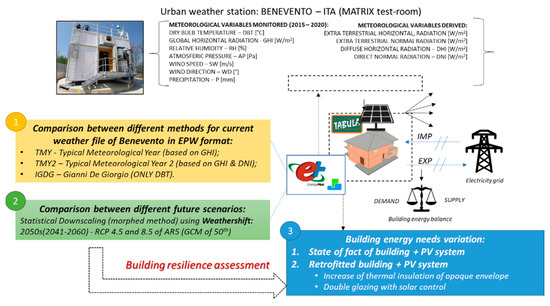
Figure 1.
Methodological approach scheme.
The construction of the weather file was based on meteorological data monitored from May 2015 to December 2020 in an urban station installed in the test-room named MATRIX—Multi Activity TestRoom for InnovatingX (41°07′54.1″ N, 14°47′03.7″ E), owned by the Department of Engineering of the University of Sannio. MATRIX is described in detail by Ascione et al. [26]. The recording of weather data was carried out by the central weather station placed on the roof of the test-room, at a height of about 7.20 m from the ground level. For the measurement of amount of rain, a rain gauge with capacity of 400 cm3 was installed. Finally, the global solar radiation and the infrared solar radiation were obtained by five pyranometers and six pyrgeometers installed on all exposures, vertical and horizontal.
As shown in Figure 1, three methodologies were compared for the construction of the weather file of Benevento because these consider the main meteorological variables in different ways. The first approach, the simplest, is related to the Italian dataset “Gianni de Giorgio” (IGDG) [27]. In this case, the construction of the typical year is based only on dry bulb temperature values by means of the calculation of average value and variance for each month on the entire population. The most representative typical month is then selected with the average value and variance of the air temperature closest to the values calculated for that month for the entire population. The typical year is finally the composition of the typical months. The other two methodologies have a more complex procedure for selecting typical months; these are the Sandia method [28], with which the typical meteorological year (TMY) is defined, and its evolution [29] (TMY2). These envisage the use of several indices obtained from the hourly values of some meteorological variables. The procedure for selecting the typical months is based on the Finkelstein–Schafer statistic, with the application of a weighting set for the considered indices. As described below, solar radiation underlies the difference between TMY and TMY2. Indeed, in the TMY2 algorithm, in addition to horizontal global radiation, the direct normal radiation was added. Moreover, starting from the TMY, two climate projections in the medium term (2050s) were generated. For this scope, two different radiative forcing values of the fifth report of IPCC [30] were examined, namely RCP 8.5 (“business as usual”) and RCP 4.5 (“strong mitigation”). The Weathershift tool [31] was used, referring to climate projections obtained with the 50th percentile global climate model (GCM). Weathershift is based on the statistical downscaling performed through the “morphing method” [32].
Considering all these weather files, the first quantitative analysis was the comparison of the different generated current and future climatic conditions. This comparison regards the main meteorological variables in term of the statistical distribution of average and extreme values. Moreover, a rigorous method for calculating heating and cooling degree days was implemented for a preliminary evaluation of the incidence on building energy consumption. In the second phase of the study, the climate files were fed to EnergyPlus 8.9 [33], through the graphical interface DesignBuilder [34] for the simulation, as a case study, of a residential building representative of the Italian stock of the 1980s. Thus, the numerical model of a single-family house was built with the information collected in the TABULA project [35,36]. The model was further customized to make it suitable for a typical Mediterranean climate such as that of Benevento. The base case also underwent several efficiency measures for the building envelope and the integration of a photovoltaic system installed on the roof was envisaged. In addition to the minimum size of 3.3 kWp, calculated in accordance with [37], the peak power was increased until the maximum size allowed by the roof surface (6.9 kWp). In the proposed analysis, for the current weather files, ∆EH and ∆EC indicate the variations of energy need for heating and cooling, respectively. Considering the future climate projections, the variations for heating and cooling energy need are indicated with ∆EH,CH and ∆EC,CH, respectively. Finally, the analysis focused only on the building energy balance in terms of electricity for the base case and the retrofitted one simulated with the TMY file and with the future climate projections. With this analysis, the resilience of the refurbished building under the expected climate change was evaluated. Moreover, the influence of future solar radiation levels both on the variation in the electricity consumption of the building and on the electricity grid as a function of the different PV production was evaluated. The differences in the building’s energy balance were evaluated, comparing the following contributions: electricity imported from electrical grid (IMP), self-consumption of electricity, and electricity exported to the grid (EXP).
3. Data and Methods for Weather File Definition
3.1. Weather Data
An EPW file (EnergyPlus/ESP-r Weather format) needs a lot of information but not all of it is mandatory for the building energy simulation tools. It is certainly essential to have the hourly values, for an entire year (8760 values), of the main meteorological variables that influence the energy needs. Thanks to MATRIX external sensors, for the purposes of this study, it was possible to have the following hourly meteorological variables:
- Dry bulb temperature—DBT (°C);
- Dew point temperature—DPT (°C);
- Global horizontal radiation—GHI (W/m2);
- Relative humidity—RH (%);
- Atmospheric pressure—AP (Pa);
- Wind speed—SW (m/s);
- Wind direction—WD (degrees);
- Precipitation—P (mm).
A simplified method for calculating the diffuse component of the global horizontal radiation (DHI) and the direct normal solar radiation (DNI) was used. This method starts from the consideration that when DHI is not directly measured, it can be calculated by the estimation of diffuse fraction of GHI (Kd) [38], where:
Kd = DHI/GHI
The Erbs regression model [39] was used, which is part of models that allow the evaluation of the diffuse fraction of GHI on an hourly basis starting from the clearness index (Kt), as follows:
Kd = 1.0 − 0.09∙Kt with 0 ≤ Kt ≤ 0.22
Kd = 0.9511 − 0.1604∙Kt + 4.388∙Kt2 − 16.638 Kt3 + 12.336∙Kt4 with 0.22 ≤ Kt ≤ 0.80∙
Kd = Kt3 + 12.336∙Kt4 with 0.22 ≤ Kt ≤ 0.80
Kd = 0.165 with Kt > 0.80
Furthermore, the technical relations (astronomical and geometric) that allowed the calculation of the hourly clearness index, starting from the hourly values of global horizontal radiation, are reported in Appendix A [38,40,41].
Finally, the direct normal radiation was obtained from the following equation [42] where θz is the zenith angle (degrees):
GHI = DNI∙cosθz + DHI
3.2. Procedures for Developing TMY and TMY2
The first TMY dataset was produced for the United States by Sandia National Laboratories in 1978 for 248 locations using long-term weather and solar data from the 1952–1975 SOLMET/ERSATZ database [28]. The National Renewable Energy Laboratory updated the TMY data in 1994 using data from the 30-year 1961–1990 [29]. In this case, the TMY methodology was changed and the new collection was identified as TMY2. The main change concerned the introduction of a tenth variable, namely the direct normal radiation to which the highest weighting factor was attributed. Recently, a new TMY series was created for Europe, with data collected from 2004 to 2018 [43]. Briefly, TMY and TMY2 are based on the variables and weights reported in Table 1.

Table 1.
Weighting factors in different TMY methods.
The reference procedure is the Sandia method, proposed below:
Step 1—For each index and month, the long-term cumulative distribution function (CDF) and the short-term CDFs were calculated. The long-term CDF uses one month of the full set of years (2015–2020 in this study), while the short-term CDF uses data from one month of just one year. The CDF for each variable is calculated by:
Herein, n is the total number of elements and k is the ranked order number (k = 1, 2, 3, …, n − 1). Next, for the choice of each typical month, the difference between the short-term CDFs and the long-term CDF were calculated for each index using Finkelstein–Schafer statistics (FS):
where m is the number of days during the month and δk is the absolute difference between long-term CDF and short-term (month under study) CDF at xk.
The FS obtained for each single year of monitoring were multiplied by the corresponding weights, obtaining the weighted statistic (WS) as in the Equation (9) where Wj is the weight assigned to the j-th index.
Step 2—From the lowest WS value, five months were identified for the choice of the typical month and these were classified based on their closeness to the long-term mean and median values of the WS.
Step 3—The persistence of mean dry bulb temperature and daily global horizontal radiation were evaluated by determining the frequency and length of runs of consecutive days with values above and below fixed long-term percentiles. For mean daily dry bulb temperature, runs above the 67th percentile (consecutive warm days) and below the 33rd percentile (consecutive cool days) were determined. For global horizontal radiation, the runs below the 33rd percentile (consecutive low radiation days) were determined. The persistence criterion excluded the month with the longest run, the month with the most runs, and the month with zero runs. The persistence data were used to select from the five candidate months the month to be used in the TMY. The highest-ranked candidate month from Step 2 that met the persistence criteria was used in the TMY. For TMY2, as a consequence of adding the index for direct normal radiation, the persistence check in Step 3 was modified to determine the frequency and run length below the 33rd percentile (consecutive low radiation days) for daily values of direct normal radiation.
Step 4—The 12 selected months were concatenated to make a complete year and discontinuities at the month interfaces were smoothed for 6 h each side using curve-fitting techniques.
3.3. Future Weather Data
The WeatherShift tool was used starting from the typical meteorological year built for Benevento. This weather generator performs a statistical downscaling based on the so called ‘morphing’ methodology, for climate change transformation of weather data, developed by Belcher, Hacker, and Powell [32]. WeathershiftTM is a generator of future meteorological files with the application of the morphing method on the offsets of 14 GCM (out of a total of 40 models). In detail, the considered models are relative to the 5th phase of the Coupled Model Intercomparison (CMIP5) project. Offsets are available for eight time periods, from the short term (2011–2030) to the long term (2081–2100), relative to the 1976–2005 baseline period and for the representative concentration paths (RCPs) 4.5 and 8.5. As reported in [31], the four closest grid points of the model were considered for each location and the offsets are calculated by performing a bilinear interpolation. The use of multiple models allows generating a cumulative distribution function (CDF) for each variable using linear interpolation between the model values. Since the offset values for each model were linked with each other, a physically consistent relationship between the values of the variables was maintained. In this study, future climate projections were generated for the time period 2041–2060 (referred to as the 2050s), for RCP 4.5 and RCP 8.5, and using the offsets on mean daily temperature change of the 50th percentiles. These future projections within the study were indicated as W4.5-50 for RCP 4.5 and W8.5-50 for RCP 8.5. It should be remembered that the RCPs are labeled after a possible range of radiative forcing values in the year 2100 (4.5 and 8.5 W/m2, for those adopted in this paper). The radiative forcing, as defined in AR4 [44], is the measure of the influence that a factor has in altering the balance of energy entering and leaving the Earth and atmospheric system. This index indicates the importance of the factor as potential climate change mechanism. The values of the radiative forcing refer to 1750, pre-industrial conditions. This tool is not made available for free to users, but it is possible to use the Weathershift online interface [45] to generate future climate projections for the selected location or starting from the file that the user provides as input.
3.4. HDD and CDD
In order to compare the hourly temperature values of examined weather files, the degree days for heating and cooling were calculated. The method reported in the standard UNI 10349-3 [46] was used. It is based on the calculation of the heating degree day (HDD) and the cooling degree day (CDD) by summing the positive differences between the base temperature and the hourly external temperature (degree-hours) and then dividing by 24. The following equations were used:
Herein, Tref is the reference temperature assumed 20 °C during the heating season and 26 °C during the summer period; Text,h is the external mean hourly temperature; and D is the total number of days (d) that are calculated considering the heating and cooling seas ons for the climate zone of interest.
4. Case Study
4.1. Base Case
The case study is a single-family house described in TABULA web-tool [36] for a middle climatic zone. This choice does not influence the results of the study, since the building is very representative of the Italian building stock of the 1980s and it will be undergoing refurbishment interventions according to the threshold value for the climatic zone of Benevento. The net heated area is 198 m2 with a gross volume of 729 m2 and the surface to volume ration is 0.65 m−1. The whole window-to-wall ratio is 8.2% with a glazed surface of 8.7 m2 on the north side and 9.7 m2 on the east side. The structure is composed of three levels: a semi-basement, used as a garage, and two floors above the ground. The building envelope is characterized by a pitched roof with brick-concrete slabs, brick wall, and double-glazed windows with air gap and wood frame. The thermal transmittance of the wall (Uw) is 0.74 W/m2 K, for the roof (Ur) is 1.20 W/m2 K, and for the slab on the ground is 1.04 W/m2 K (Us); the solar factor (SF) and the glass thermal transmittance (Ug) of the windows are, respectively, 0.75 and 2.08 W/m2 K. The insulation level is very low if it is compared with the current Italian requirements [47] for Italian Climatic Zone “C”. Indeed, in case of refurbishment works, the thermal transmittance must be lower than 0.36 W/m2 K for the walls, 0.38 W/m2 K for the basement, 0.32 W/m2 K for the floors, and 2.00 W/m2 K for the windows. Regarding the plants, a gas boiler with atmospheric burner and chimney lower than 10 m, placed in an unheated room, is used for heating service. It produces hot water at 80 °C for radiators placed in every room. The domestic hot water is produced by the same boiler coupled with a storage tank with a medium level of insulation. The total efficiency of the gas boiler was set equal to 0.9. For the summer air conditioning, it was assumed that in the main room, a split-system was installed with a nominal cooling capacity of 3.25 kW and a nominal performance coefficient equal to 3.0. The lighting system consists of fluorescent lamps with a specific rated power of 5.0 W/m2. In the heating season, a set point temperature of 20 °C was set with an operating period (10 h per day) from 15 November to 30 March, as defined in [24,25]. In the cooling season, from 1 June to 30 September, the set-point temperature is 26 °C (10 h per day). For the photovoltaic system, the use of monocrystalline silicon modules was considered, with an area of 1.63 m2, peak power of 300 W, and module efficiency of 18.4%. The technical data comply with a SUNPOWER model (SPR-300-WHT-I) [48]. The model rendering is shown in Figure 2A and the description of the main data for the thermal zone is reported in Figure 2B, which also shows the distribution for the 2nd floor. The infiltration and ventilation rate was fixed globally to 0.5 ACH. The simulation of this configuration represents the state of fact of the building (base case).
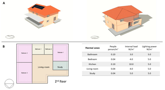
Figure 2.
Case study: (A) building rendering; (B) thermal zone.
4.2. Energy Retrofit Measures
To improve the building envelope performance, the thermal insulation of the external walls and the roof was considered (TI in the following) in accordance with the Italian Ministerial Decree 26 June 2015 [47]. In both cases, the thermal insulation layer was applied on the external side; it consisted of rockwool panels (6.0 cm) for the external walls (Uw = 0.34 W/m2 K) and 10 cm of expanded polystyrene (EPS) for the roof (Ur = 0.33 W/m2 K). Moreover, the installation of a solar control double-glazing system was considered; in this case SF was 33% with transmission in the visual range of 70% and Ug was equal to 1.00 W/m2 K.
5. Results and Discussion
5.1. Application of Different Methodologies for the Typical Year
Table 2 shows the set of data for the choice of the typical months for the IGDG weather file. The absence of some values is due to temporal phases not included in the multi-year monitoring or to anomalies in the data detection of the weather station. The variance (σ2) identifies the dispersion of the hourly temperature values around the calculated monthly average value (µ). The months with the average value and variance of the dry bulb temperature closest to the values calculated for that month on the entire population were chosen. These data help to understand the implications of the IGDG methodology. For instance, in December, the year closest to the long-term values was 2018; however, there is a sensible variation with the value calculated during the other years. For the summer period, July was the month for which the mean value was most comparable in the analyzed years except 2015, during which there was a higher value (27.1 °C).
Table 2.
Mean and variance values in each month of dry bulb temperature for each month.
In some months, the variance was very high, for instance in December and January mainly during 2016 but also for the spring months during 2017. This means that the external conditions are extremely variable and the adoption of the mean value could be not representative of the real conditions.
Table 3 shows the year selected in each month for the definition of the typical year with the selected methods.
Table 3.
Composition of typical meteorological years.
Another interesting comparison regards the methodologies based on the original and modified Sandia method (TMY and TMY2). For instance, with TMY, August 2019 was chosen as the typical month. As can be seen in Figure 3A, in this year, the short-term CDF had FS equal to 0.08 compared to the long-term CDF for GHI. In many points, there was a strong proximity of the cumulative distributions. For the same month of the same year, as seen in Figure 3B, the short-term CDF of the DNI denoted a greater discrepancy than the long-term CDF with FS equaling 0.20. This comparison shows the differences between the two methods and thus it can be concluded that the typical months chosen for TMY2 had a greater agreement between the chosen DNI and the one of the baseline multiyear record. This aspect is not trivial since the direct normal radiation has high weight when a renewable energy system, such as a photovoltaic system, must be considered. Moreover, it also influences the solar gains contributed in the building energy balance and mainly in the summer period, it could affect the evaluation of overheating inside the building and the cooling consumptions.
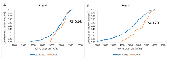
Figure 3.
CDFs comparison in August: (A) GHI; (B) DNI.
Table 4 shows the incidence of the weighting factors for August 2019. The calculated WS was equal to 0.104 and 0.128 for TMY and TMY2, respectively. Thus, TMY and TMY2 determine a different outcome in the final steps of their composition procedure, leading, in many cases, to the choice of different typical months.
Table 4.
FS and WS calculation for weather indices in TMY and TMY2—August 2019.
5.2. Preliminary Analyses on Current Climate Files
Figure 4 shows the comparison of the methodologies used for the construction of the “current” climate files of Benevento, for the distributions of the hourly values of DBT (Figure 4A) and GHI (Figure 4B). The first unexpected conclusion is that the statistical distributions seem comparable in both cases.
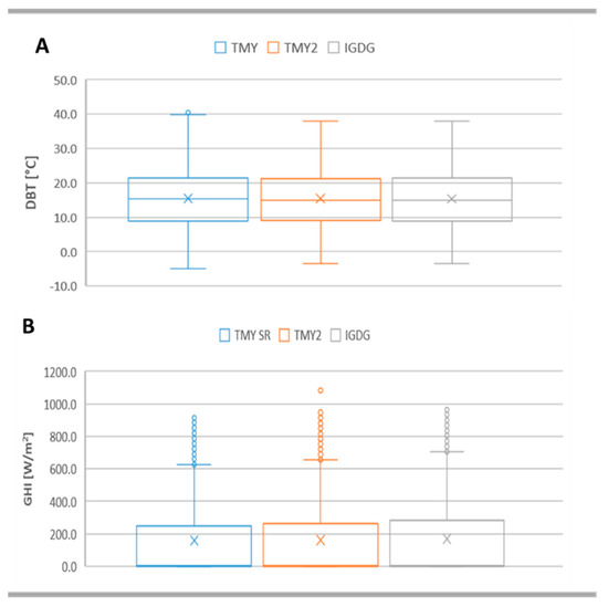
Figure 4.
Current weather files of Benevento: (A) DBT; (B) GHI.
However, it is important to remark that these are global distributions and thus the extreme values can occur in different hours, days, or periods, and this influences the resolution of the heat balance on the building. Considering the temperature, TMY presents a distribution with greater variability over the year. The average value is equal to 15.3 °C while the maximum and minimum values are, respectively, 39.9 °C and −4.9 °C. Furthermore, it is the only one to contain an aberrant value, equal to 40.5 °C. It can be concluded that with the Sandia method, the typical climatic year of Benevento was generated with more extreme conditions.
The box-plots of Figure 4A for TMY2 and IGDG are comparable, with the same maximum and minimum values, respectively, 38 °C and −3.5 °C, and an almost coincident average value. This is very significant considering the strong differences in the methodologies. The values relating to the first and third quartiles are instead comparable for all three distributions and, on average, equal to 21.4 °C and 8.9 °C, respectively. Regarding the horizontal global radiation (Figure 4B), the distribution of IGDG is the one characterized by the highest values. The average value of IGDG is equal to 168.2 W/m2 while those relating to TMY2 and TMY are equal to 162.1 W/m2 and 158.6 W/m2, respectively. Instead, the maximum value observed with IGDG, without considering the aberrant values, is equal to 705 W/m2 while these are 655 W/m2 and 626 W/m2, respectively, for TMY2 and TMY. Therefore, the box-plots on GHI also show greater comparability between the distributions of TMY2 and IGDG. It seems that TMY is built with one or more typical summer months with lower solar radiation levels.
Figure 5A shows the calculated heating degree days and in Figure 5B, the CDDs are presented. In both cases, the values are comparable with a maximum difference of 3.2% for HDDs and 5.1% for CDDs between TMY and TMY2.
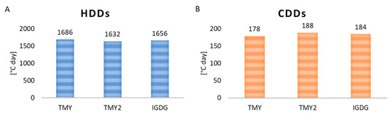
Figure 5.
Degree days: (A) HDD; (B) CDD.
The current evaluation of the energy performance for the Italian normative is based on the HDD and it does not consider the CDD. Thus, the heating degree days (1316 HDD) according to the decree n° 412/1993 [25] can be considered for some other evaluations. Considering the value calculated from TMY, there is an increase of +28.1%. This discrepancy is both due to the adopted dataset (not updated weather data) and to the methodology, since for the value included in the National Decree, the average daily temperature is used in the calculation of the HDDs. It is clear that the actual adopted indicator is not able to describe the variation in the heating performance of a building due to colder conditions implemented in the old data that do not take into account climate changes.
5.3. Comparison of Future Climate Files
Figure 6A shows the comparison between the distribution of DBT in case of TMY and for the projections obtained starting from TMY with the WeatherShift tool. It was interesting to observe that the variation in the average annual values depended both on the effects of climate change but also on the uncertainties of the projections that different models considered for the same time horizon. In the cases of W4.5-50 and W8.5-50, the average temperatures were about +12% and +15% compared to the average value of TMY, respectively. Even the extreme values of the distribution underwent an evolution. The minimum value went from −4.9 °C to −3.4 °C with the “strong mitigation” scenario (RCP 4.5) and to −2.8 °C with the “business as usual” scenario (RCP 8.5). The maximum values without considering the aberrant ones, were comparable, and near 44 °C in both cases. Similar conclusions can be arrived at for DNI distribution, shown in Figure 6B.
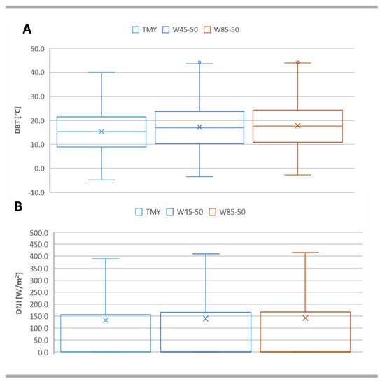
Figure 6.
Current weather file and climate projections: (A) DBT distribution; (B) DNI distribution.
The average value for TMY was about 132.3 W/m2, while it increased up to 139.6 W/m2 with RCP 4.5 and up to 142.2 W/m2 with RCP 8.5. The maximum values of the distributions were equal to 389 W/m2, 411 W/m2, and 416 W/m2 for TMY, W4.5-50 and W8.5-50, respectively. The increase obtained for DNI is in accordance with the study by Huber et al. [49]; their calculations indicate that future (2035–2039) surface irradiances in Europe and Australia are likely to be increased compared to the past (1995–1999) by about +10% in DNI and some 1–5% in GHI. These variations are attributable to the effect of multiple atmospheric data that influence the surface irradiance, i.e., clouds, aerosols, surface albedo, and water vapor.
In general, despite the uncertainties connected to the considered projections, a future transition towards a dominant cooling climate for Benevento can be certainly concluded. The estimated values of heating and cooling degree days (Figure 7) clarify this point.
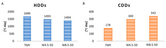
Figure 7.
Degree days for future projections: (A) HDD; (B) CDD.
The HDD reduction was higher in the case of “business as usual” scenarios (−17%) as well as the increment of the CDDs, which was almost double compared with the current condition. The result in terms of CDD was in accordance with the expected increase in the external temperature. The comparison of the monthly mean temperatures for TMY and W8.5-50 indicated that the maximum monthly average temperature variation occurs in June. In this month, the average value of W8.5-50 is equal to 25 °C, while the average values of W4.5-50 and TMY are equal to 21.4 °C and 24.6 °C, respectively. When the daily average temperature is considered, the difference between TMY and W8.5-50 varies from 1.3 °C to 9.3 °C. The hottest month is August and, in this case, the average temperature is 26.8 °C for TMY, 29.1 °C with W45-50, and 30.1 °C with W8.5-50. In that month, considering the daily average temperature, there is a difference between TMY and W8.5-50 that varies from 1.1 °C to 3.4 °C. Moreover, the results are comparable with those obtained for other zones. For instance, Ramon et al. [50] concluded for Belgium that the HDDs will decrease by around 27% and the CDDs will increase with a factor of 2.4 in the RCP 8.5 scenario. The obtained result is also consistent with respect to the projections of [51]. They found that in southern Europe, the HDDs (considering a base temperature of 15 °C) will decrease from −30% (RCP 4.5) to −35 % (RCP 8.5); instead the CDDs (considering a base temperature of 22 °C) will increase more than 40% with the RCP 8.5 scenario.
5.4. Energy Simulation Results
Three analyses are proposed for the simulation results: a sensitivity analysis on the PV production by varying the size and the weather data; the comparison of the energy needs for heating and cooling both of the base case and the retrofitted building with different weather data; and the electricity balances of the building to verify its resilience when subjected to the refurbishments intervention.
5.4.1. Comparison of PV Production
Figure 8 shows the monthly production from PV obtained with TMY for the four examined sizes. The equivalent one-diode was used in DesignBuilder. Mathematically, the PV module employs equations for an empirical equivalent circuit model (a DC current source, diode, and either one or two resistors) to predict the current-voltage characteristics of a single module. The strength of the current source is dependent on solar radiation and the characteristics of the diode are temperature-dependent.
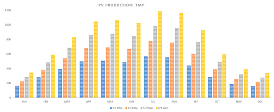
Figure 8.
PV production with TMY by varying the system’s size.
The electricity generation linearly increases with the installed size. When the peak power is 3.3 kWp, the maximum value is observed in July, 490 kWhel, while the minimum occurs in December and it is equal to 160 kWhel. Among the months of the heating season, the highest PV generation occurs in March (around 397 kWhel). In January, the observed value is comparable with December, while in February there is an increase of about 71% compared to the previous months. Among the intermediate months, the production of electricity in April and May is much higher than that obtained in October and in September. For instance, with the minimum peak power value, the PV production in May is approximately 508 kWhel while in September and October it is lower, respectively, by −13% and −42.8%. By increasing the peak power, the same percentage variation of PV production is observed in each month. Therefore, from 3.3 kWp to 4.5 kWp, the simulated electricity generation increased by 36.4%. With 5.7 kWp, the PV production increased by 74% in all months. Finally, with the maximum size (6.9 kWp), the simulated electricity generation showed a monthly increase of about 109% compared to the minimum peak power.
The same conclusion is true for the simulation results with the other two current climate files. Indeed, even if the monthly electricity production values obtained with TMY2 and IGDG are different from those observed for TMY, it can be seen that the relationship between the values observed with the minimum system size and the subsequent sizes is linear and the values of the Y-axis intercept are negligible in each equation (Figure 9). Therefore, the slopes of the relations with the same peak power leap of the photovoltaic system demonstrate the same monthly percentage increment of the PV production. This certainly means that, at least for the case study, the simulated model is not influenced by the input climate file in term of percentage variations of photovoltaic production. There is only a dependence in the size variation. At the same time, this also means that, with the same peak power of the PV system, the monthly percentage variations of photovoltaic production between one climate file and another are constant.
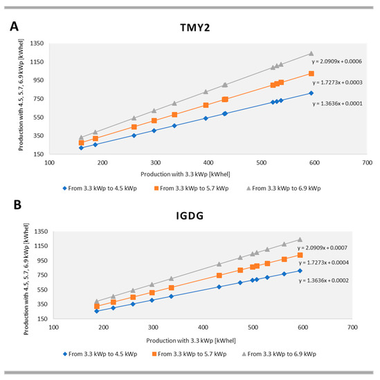
Figure 9.
Correlation between PV productions as the system size varies: (A) TMY2; (B) IGDG.
Figure 10, considering the peak power of 3.3 kWp, summarizes the percentage variation (ΔEPV,tmy) of PV production with the current weather files (Figure 10A) and with the future projections (Figure 10B) compared to TMY. For instance, in January, the electricity generations obtained with TMY2 and IGDG are the same and increased by about 57% compared to that obtained with TMY in the same month (Figure 10B). During the heating months, TMY2 and IGDG show the same ΔEPV,tmy; this also happens in February and March, respectively equal to 5.8% and 9.1. In November, there are no differences between the examined files. In December, TMY and TMY2 give the same production while for IGDG, ΔEPV,tmy is +37.2%. In the summer months, both IGDG and TMY2 show the highest percentage change in June, respectively +14.9% and +6.5%. In July and August, ΔEPV, tmy is respectively equal to +4.7% and −4.6% for both TMY2 and IGDG. In April and May, there are no differences between the PV production of TMY and IGDG while in the case of TMY2, ΔEPV,tmy is −20.9% and +5.8%, respectively.
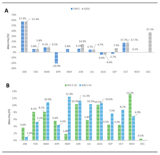
Figure 10.
Percentage variations of PV production vs. TMY: (A) TMY2 and IGDG; (B) W4.5-50 and W8.5-50.
When the differences in the prevision are not observed, it means that the same month was selected for the definition of the typical year. However, the consideration of different weight and variables led to different estimations in the producibility of the PV-system; this can influence the building energy balance.
For the future scenario, the values of ΔEPV,tmy are always positive (Figure 10B) but with W8.5-50, ΔEPV,tmy is not always higher than in W4.5-50 scenarios, mainly during the winter months. For instance, in November, ΔEPV,tmy is +13.2% and +6.9% with the W4.5-50 and W8.5-50, respectively. In January, the percentage changes observed with future projections are very low while they are practically negligible in December and this finding could indicate that the emission scenario slowly affects the solar radiation of winter months. In the summer months, the percentage variations are comparable in June and in August. In July, ΔEPV,tmy is +5.8 and +10% with the W4.5-50 and W8.5-50, respectively; thus with the assumed emissions scenario, there is a sensible increase in the photovoltaic producibility that can positively influence the building energy balance.
It can be also noted that the expected future values of PV production are closely linked to how the statistical downscaling carried out on the TMY file changed its distributions concerning solar radiation. Table 5 shows, both for TMY and for future climate projections, the mean expected value and the standard deviation of photovoltaic producibility in each month. These indices were calculated starting from the total daily PV production obtained with the peak power of 3.3 kWp. In general, there were no large differences in standard deviation in each month between TMY and future projections. Indeed, the downscaling varied according to the same criterion, the hourly values of solar irradiation. Between the winter months, the average expected values are highly comparable with the average values of TMY, mainly in January and December. In February, April, and November, the average value expected with W4.5-50 is higher than the value obtained with W8.5-50, despite the RCP 8.5 scenario being less optimistic than the RCP 4.5 scenario. In the summer months, the expected future changes in PV production are more evident, compared to TMY. For example, in June, in terms of mean value and standard deviation, there is a variation from 16.3 ± 3.5 kWhel with TMY to 18 ± 3.8 kWhel with W4.5-50 and to 18.2 ± 3.8 kWhel with W8.5-50. In July, the mean expected value with W8.5-50 is the highest. This value is increased by 4.2% compared to the average value of TMY in the same month and by 10.3% compared to the mean value expected with W4.5-50.
Table 5.
Mean and standard deviation of PV production: TMY and climate projections.
5.4.2. Energy Need Analysis
Considering the base case, Figure 11 shows the heating and cooling thermal energy need by varying the weather file. In the heating season, the energy requirements obtained with TMY2 and IGDG are strongly comparable in all months, reporting similar percentage differences compared to TMY (Figure 11A). Therefore, the IGDG method also seems to be a reliable method despite it being based exclusively on the dry bulb temperature values in the choice of the typical months. The higher difference is the thermal energy request in January (+32.5%). February is the only winter month in which the heating energy needs obtained with TMY are lower than those obtained with TMY2 and IGDG, respectively by 13.4% and 15.7%. In March, the heating energy needs obtained with TMY are on average 21.5% higher than the results obtained with IGDG and TMY2 in the same month. On the other hand, the differences in energy requirements observed in November and December are negligible. Yearly, the energy needs for heating are equal to 32 kWh/m2 year in the case of TMY and it is increased by 10% compared to TMY2 and by 9.8% compared to IGDG.
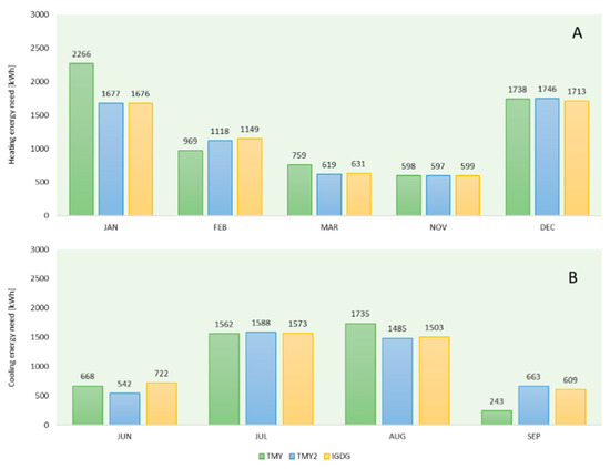
Figure 11.
State of fact—energy need with current climate files: (A) heating; (B) cooling.
The different criteria for selecting the typical months lead to higher differences in the cooling season, mainly in June and September (Figure 11B). In June, the value obtained with the IGDG is higher by 8% compared to TMY and 33.21% compared to TMY2. September is a very particular case. Indeed, in this month, the energy needs for cooling obtained with TMY are reduced by 63.3% compared to TMY2 and 60.1% compared to IGDG, while, as seen previously, comparable results were observed in terms of photovoltaic generation and CDDs. Globally, the energy needs for cooling are equal to 21.2 kWh/m2 year with TMY, 21.6 kWh/m2 year with TMY2, and 22.3 kWh/m2 year with IGDG.
The energy needs of the building with the energy refurbishment and the calculated energy savings are shown in Figure 12, for the current climate files. The energy needs for heating become 23.1 kWh/m2 year with TMY, 21.3 kWh/m2 year with TMY2, and 21.5 kWh/m2 year with IGDG. The proposed passive measures are able to reduce the energy requirements with comparable savings for all three files. In January, the month with the highest energy requirements, ΔEH is −28.1% with TMY while it is equal to −25.9% for both TMY2 and IGDG. The reduction in energy needs for cooling is mainly due to the installation of double glazing with solar control. However, thermal insulation also contributes to improving summer energy performance of the case study since the insulating layers also contribute to increasing the inertial properties of the opaque building envelope, since significant thicknesses of the insulation are required. Globally, the cooling energy demand is equal to 14.3 kWh/m2 year with TMY, 14.6 kWh/m2 year with TMY2, and 14.8 kWh/m2 year with IGDG. The largest reductions in the cooling season are observed in June. In this month, ΔEC is −40.2%, −41.9%, and −42.4% with TMY, TMY2, and IGDG, respectively. Thus, it can be concluded that the variation in the energy prevision of the base case causes comparable variation in the energy performance after the refurbishment and the obtainable savings are comparable.
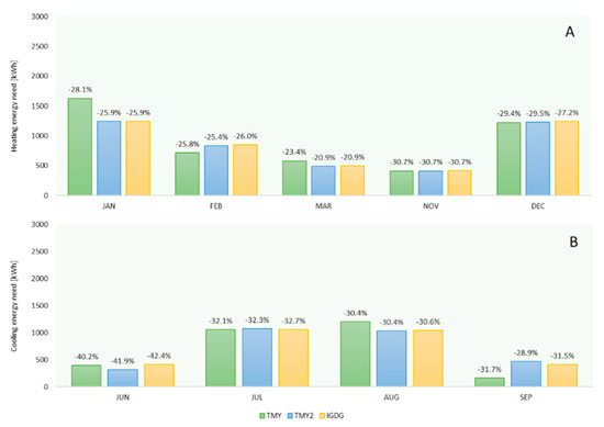
Figure 12.
Retrofit—Energy needs with current climate files: (A) heating; (B) cooling.
Figure 13 shows the percentage changes obtained with the future climate projections generated from TMY. The values of ΔEH,CH and ΔEC,CH are calculated with respect to the energy needs of the retrofitted building simulated with TMY. This index allows estimating the potentiality of a retrofit action designed for the actual performance and climatic conditions along the years; thus, it can be considered a measure of resilience of the building refurbishment. First of all, the energy saving calculated for the winter months must be attributed both to the efficiency measures and to climate changes, because as demonstrated in Figure 6, the HDDs tend to decrease. As expected, the percentage reductions in the heating energy needs are always higher for the “business as usual” scenario (Figure 13A). On the other hand, for the cooling season (Figure 13B), the retrofit interventions seem to not be resilient for the expected climate changes. Indeed, the cooling demand increases, mainly in the “business as usual” scenario, due to the radiative forcing and temperature increase. These lead to higher levels of irradiation, as previously discussed, and consequently this affects the amount of internal solar gains that can reduce the heating energy demand and increase the cooling energy demand.
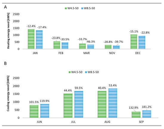
Figure 13.
Retrofit—Energy needs of future climate projections: (A) heating; (B) cooling.
These results are comparable with those obtained by Tootkaboni et al. [52] for Italy. They have found that for refurbished buildings, the cooling demand could vary between 29% and 117% and the heating demand could decrease between −12% and −38%.
5.5. Energy Building Balance
5.5.1. State of Fact with Minimum PV System Size
The previous analysis underlined that, along with the application of energy efficiency measures able to reduce both the heating and cooling needs, with the selected emission scenario, the cooling demand will increase until the 2050s. For the case study, the energy needs for cooling are met by an electric split system. Therefore, the building’s electricity balance is certainly penalized by climate change since the consumption of electricity for cooling is bound to increase over time. For this reason, it is interesting to understand how photovoltaic system integration can improve the building’s electricity balance and thus the summer energy performance.
For the size 3.3 kWp and base case, Figure 14, Figure 15 and Figure 16 report the energy balances of the building based on the simulations carried out with TMY, TMY2, and IGDG. For instance, in January, February, and March with TMY, the self-consumed electricity corresponds to 12%, 17%, and 24% of total electricity consumption, respectively. In the same months, with both TMY2 and IGDG, the percentages are 16%, 21%, and 27%. In January, as already observed, the electricity generation obtained with TMY2 and IGDG increased by about 57% compared to TMY. For this reason, with the same total electricity consumption, the simulations made with TMY2 and IGDG in January compared to TMY highlights a significant increase in the exported electricity (+88%).
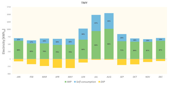
Figure 14.
Energy balance with TMY simulations results—base case with 3.3 kWp.
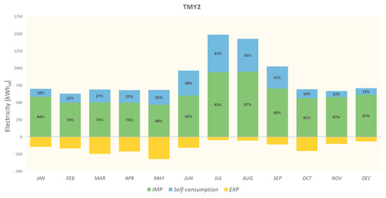
Figure 15.
Energy balance with TMY2 simulations results—base case with 3.3 kWp.
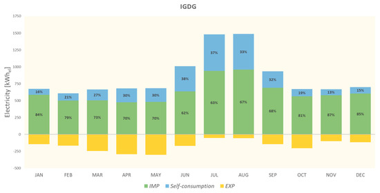
Figure 16.
Energy balance with IGDG simulations results—base case with 3.3 kWp.
This result is significant, since the climate files, created starting from the same baseline period but based on a different procedure for selecting the typical months, lead to different observations in January both in terms of exported electricity (renewables energy) and in terms of the electrical grid impact. In the summer months, the total electricity consumption of building is different with the created files. However, the percentage of self-consumption remains comparable. For example, in June, the total electricity consumption is 1027 kWhel, 965 kWhel, and 1031 kWhel with TMY, TMY2, and IGDG, respectively. The percentage of self-consumed energy is 36% with TMY and 38% with TMY2 and IGDG. The highest contribution of electricity exported in this month is with IGDG and is equal to 170 kWhel. This value increased by 7.7% compared to the electricity exported in the same month with TMY2 and by 45.8% compared to TMY. Therefore, the strong similarities between TMY and IGDG in terms of electricity consumption are not confirmed in terms of electricity exported due to the different electricity generation from photovoltaics in the same month. However, it was noted that a 15% difference in photovoltaic generation translates into a 45.8% difference in terms of exported electricity. In July, the self-consumption represents the highest percentage of total electricity consumption, equal to 37% with all examined climate files. In August, the highest electricity consumption is obtained with TMY, equal to 1544 kWhel. Compared to this value, those obtained with TMY2 and IGDG are reduced by 8.3% and 7.2%, respectively. The percentage of self-consumption is 34% with TMY and 33% in the other two cases. Regardless of the climate file used, in the months of July and August, the increase in electricity consumption for cooling is coupled with an increase in the generation of electricity from photovoltaics and the resulting effect involves a maximization of self-consumption and a minimization of electricity exported to the electrical grid. September is included between the months of the cooling season. As previously seen with the cooling energy needs, the typical month chosen for TMY is certainly characterized by lower levels of temperature and solar radiation than TMY2 and IGDG. In detail, with TMY, the total electricity consumption is equal to 839 kWhel and it is covered with in situ production while the energy exported is equal to 229 kWhel. In the case of TMY2 and IGDG, the total consumption of electricity increases by about 21% compared to TMY and self-consumption covers about 31% and 32%, respectively.
Considering the building simulated with TMY, when the installed power goes from 4.5 kWp to 6.5 kWp, as expected, the self-consumption of the total electricity consumption increases. In detail, compared to the results with the power of 3.3 kWp, previously discussed, self-consumption shows an average monthly increase of 20% with 4.5 kWp, 35% with the 5.7 kWp size, and 47.2% with the 6.9 kWp. In the summer months, the amount of self-consumed electricity is always the highest. In July, self-consumption covers 44.9% of total electricity consumption of building with a 4.5 kWp size and 55% with the maximum peak power. Compared to the minimum size, with the same electricity consumption of the building, self-consumption increases by 23% with 4.5 kWp, by 38% with 5.7 kWp, and by 51% with 6.9 kWp. Maximizing the power of the photovoltaic system therefore leads to the greatest benefits since the building imports the minimum amount of electricity, with an average monthly reduction of about 16% and a maximum reduction in July, equal to −29.3%. At the same time, the increase in the peak power of the PV system installed on the building roof produces inevitable increases in electricity exported to the grid. The average monthly increase compared to the minimum size is 90 kWhel with 4.5 kWp, 193 kWhel with 5.7 kWp, and 303 kWhel with 6.9 kWp. On a monthly basis, it was noted that the highest values of exported electricity occur in the months of April and May, with negligible differences. For instance, in May, it goes from 147 kWhel with 4.5 kWp to 465 kWhel with 6.9 kWp. In these intermediate months, the building is not air-conditioned but, due to the climate in question, the levels of solar radiation and air temperature are comparable to the months of the cooling season. However, it is necessary to take into account the impact on the electricity grid linked to the higher peak power of the system. This aspect is not insignificant, especially if we consider that we are moving towards an increasing penetration of distributed photovoltaics with consequent voltage problems at low and medium voltage grid levels.
Finally, in Figure 17 and Figure 18, the yearly results are reported, comparing the three climate files used for the dynamic simulation. The annual values are obtained by solving the electricity balance of the building in each month and adding the obtained contributions. In terms of imported electricity, there is an average reduction of 7.6% going from 3.3 kWp to 4.5 kWp, of 6.2% going from 4.5 kWp to 5.7 kWp, and of 5.1% going from 5.7 kWp to 6.9 kWp for all files. Furthermore, the values calculated with TMY are always the highest; the differences with TMY2 and IGDG increase as the area of the photovoltaic modules increases. In particular, going from the minimum peak power to the maximum one, the percentage increase of electricity imported from the grid, simulating with TMY, goes from +1.27% to +2.38% compared to the TMY2 values and from +1.10% to +2.41% compared to the IGDG values. In terms of electricity exported, the simulations with IGDG show the highest values on annual base, with an average increase of 2.4% compared to TMY and 9.8% compared to TMY2. On average, the electricity exported to the grid on an annual basis increases by 60.6% passing from 3.3 kWp to 4.5 kWp power, by 43% passing from 4.5 kWp to 5.7 kWp and by 32.3% passing from 5.7 kWp to 6.9 kWp.
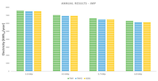
Figure 17.
Imported electricity—annual results of current weather files.
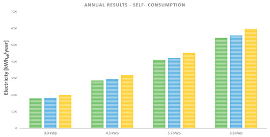
Figure 18.
Self-consumption—annual results of current weather files.
5.5.2. Energy Balance with Retrofit Scenario
To analyze the results of the retrofit configuration, in terms of the building’s energy balance, only the months of the cooling season can be considered, since the variations in the power consumption of the auxiliary devices serving the heating system are negligible. Figure 19, for the simulations carried out with TMY, shows the energy balance for the retrofitted building by varying the size of the PV system.
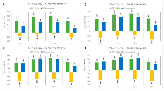
Figure 19.
TMY—Results with retrofit scenario: (A) 3.3 kWp; (B) 4.5 kWp; (C) 5.7 kWp; and (D) 6.9 kWp.
The percentage variations are referred, for each peak power, to the simulations result of the base case, with the same size of PV system. It can be observed that the percentage variations of imported and self-consumed electricity are comparable passing from the state of fact to the retrofit scenario, for each size. In August, self-consumption is reduced by 6.0% with 3.3 kWp (Figure 19A) while it is reduced by 14% with the maximum size (Figure 19D). The opposite effect is observed with electricity imported from the grid. Compared to the base case, the maximization of photovoltaics combined with the refurbishment intervention leads to a reduction of imported electricity. With the same electricity consumption, the maximum peak power increases the self-consumption in each month. For instance, in July with the minimum power of the photovoltaic system, the self-consumption is equal to 496 kWhel; it increases by 18% with 4.5 kWp, 32% with 5.7 kWp, and 41% with 6.9 kWp. Furthermore, the simultaneous reduction imported electricity and self-consumption causes the increase of the energy exported to the grid, compared to the base case. In particular, in July and August (Figure 19A), the exported energy goes from 108 kWhel to 174 kWhel (+77%) with 4.5 kWp, from 228 kWhel to 315 kWhel (+32%) with 5.7 kWp, and from 368 kWhel to 468 kWhel (+44%) with the maximum size of PV system. The highest value occurs in all cases in September which is the summer month characterized by the lowest self-consumption and by a contribution of imported energy comparable to June. In the case of the maximum power of the PV system, the electricity exported to the grid is equal to 596 kWhel, i.e., +8.4% compared to that exported in June, + 4% compared to the non-retrofitted building, and +29.3% compared to electricity exported in the same month with a 5.7 kWp photovoltaic system for the retrofitted building. It is important to remark that this analysis does not take into account the loss in the efficiency of the PV system within a service life of 30 years. However, some studies like [53] suggest that the impact of climate change on PV systems varies up to 2.5% but it could be mitigated through proactive design and the application of maintenance strategies. Thus, the proposed analysis is the first attempt to evaluate what happens to the building’s energy balance. In further research, a loss assessment curve will be implemented for the dynamic evaluation of the energy efficiency reduction both of the PV system and the building envelope components. Moreover, an economic analysis will be performed to study the incidence on the operating costs by also taking into account the maintenance and replacement.
5.5.3. Building Resilience Assessment
The monthly energy balances obtained with the medium-term projections are reported below for evaluating how climate change affects the energy balance of the retrofitted building. In particular, the aim of this analysis is to understand which peak power of the PV system is most suitable to allow the retrofitted building to cope with the effects of the expected climate change. The maximum and minimum values of the peak power of the PV system are taken into consideration. Starting from the case with 3.3 kWp, both for the “strong mitigation” future scenario (Figure 20A) and the “business as usual” scenario (Figure 19B), there are no important variations of the imported and self-consumed electricity in the winter and intermediate months. Furthermore, in these months, the increased PV production leads to an average percentage increase of exported electricity, equal to 7% with RCP 4.5 and 8% with RCP 8.5. Among the intermediate months, the two future scenarios show the greatest differences in May. Indeed, compared to TMY results, the exported energy shows an increase of 2% with W4.5-50 and of 16% with W8.5-50. In the months of the cooling season, in addition to the different PV production, there are the effects of changes in energy needs. Compared to the simulation with the current climate file, both the electricity imported from the electricity grid and self-consumption increase, mainly with the “business as usual” scenario. For instance, in July, the retrofitted building imports 929 kWhel (+21%) with RCP 4.5 and 983 kWhel (+28%) with RCP 8.5. The energy exported to the grid should decrease in the months of July and August. In general, the expected minimum power results in very low levels of electricity exported in all months. At the same time, the building is unable to cope with the increase of consumption in the summer months. Different conclusions can be found with the highest peak power in Figure 21. In this case, the high electricity generation from photovoltaics allows counterbalancing the imported energy since the increase in self-consumption prevails. At the same time, the energy exported to the grid in the summer months reaches acceptable values, lower than the values observed in February and March. For instance, in August, the electricity imported from the grid in the case of W4.5-50 (Figure 21A) goes from 967 kWhel with 3.3 kWp to 690 kWhel with 6.9 kWp. Therefore, imported electricity is reduced by about 29%. At the same time, with the “business as usual” scenario, the imported energy varies from about 1044 kWhel to about 729 kWhel (−30%).
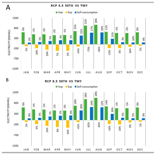
Figure 20.
Retrofit scenario and 3.3 kWp: (A) RCP 4.5 vs. TMY; (B) RCP 8.5 vs. TMY.
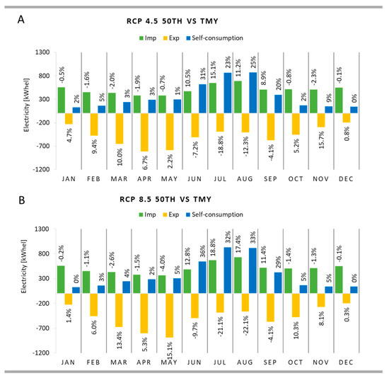
Figure 21.
Retrofit scenario and 6.9 kWp: (A) RCP 4.5 vs. TMY; (B) RCP 8.5 vs. TMY.
Even if compared to the simulated retrofit scenario with TMY, the energy imported in future scenarios is higher; with the maximization of PV production, it could decrease since the expected climate change favors the increase of electricity consumption in summer months and thus self-consumption. The increment of installed power seems suitable for improving the resilience also when the size is overestimated for a single-family building. The installation of a storage system could minimize the imported energy with respect to TMY since self-consumption would further increase. At the same time, the introduction of a storage system could help to reduce the amount of exported energy that could represent a problem in terms of impact on the national grid. Moreover, it can also be underlined that due to the increasing levels of temperature and solar radiation shown by the emission scenarios, April and May would also be included in the cooling season and with the maximization of installed power, the electricity consumption could be almost entirely covered by the in situ production. Indeed, the current methodology [54] for establishing the duration of the cooling season is based on the ratio between the monthly (or hourly) heat losses and heat gains that depend both on the external conditions and on the building characteristics. Considering the increment of CDD, it is presumable that for a given building, this ratio will go up and thus the cooling season will be extended. The same methodology is also given for the winter season by taking into consideration the ratio between heat gains and heat losses, and it is expected that this value can match the limit for more time and the duration of the heating season will increase. However, in the winter season, the prescriptions of the Italian Decree [25] must also be considered.
6. Conclusions
The paper investigated the implications of different methodologies aimed at creating the weather files to be used for the building energy performance simulation. First of all, the most representative variables, the solar radiation and the air temperature, were compared with a statistical approach both considering different methods for selecting the typical months and the effects of climate changes. This analysis indicated that the statistical distributions of the hourly values of the dry bulb temperature and global solar radiation are comparable with all considered methods, but the extreme values can occur in different hours or days; this influences the resolution of the building heat balance. When the climate changes were considered, marked transition towards a dominant cooling climate for Benevento was found. Indeed, in the case of “business as usual” scenarios, the HDDs would be reduced by −17%, while the CDDs would be almost double compared with the current condition. Indeed, the daily average temperature is expected to be higher from 1.3 °C to 9.3 °C in a typical month as June.
The simulation results for the base case and the retrofitted building suggest the following conclusions:
- The monthly electricity production with different methodologies can vary from 4.7% (June) to 57% (January) and the same variations are observed when the installed peak power changes. When the climate changes are considered, the PV production increases in each month with maximum variation of 12.4% (May) with RCP 8.5 and 13.2% (November) with RCP 4.5.
- The application of passive energy efficiency measures is not able to front the increase of the cooling demand until the 2050s; e.g., in July, the cooling request increases by 44% with RCP 4.5 and of 60% with RCP 8.5. In the cooling season, the climate changes would cause the increment of both imported electricity and self-consumption; thus the maximization of the installed peak power allows improving the building resilience.
The proposed study is the first attempt to evaluate the incidence of climate change on building energy balance when renewable production is considered. However, further analysis is needed for proposing a whole optimization of the design. Indeed, the changes in the external temperature could be used with a bioclimatic approach for maximizing the passive control of indoor conditions. Then, the interaction with the electricity grid has to be studied because the in situ storage is needed in order to avoid the imbalance of the national electric system in some periods of overproduction, due to the maximization of installed peak power. Moreover, future research will be also focused on other climates and types of building, in order to generalize the conclusion of the adopted methodology.
Author Contributions
Conceptualization and methodology, G.P.V. and R.F.D.M.; formal analysis, investigation, data curation, A.G., V.F. and M.M.; writing—original draft preparation, S.R. and R.F.D.M. All authors have read and agreed to the published version of the manuscript.
Funding
This research was funded by PRIN 2017 for the project titled SUSTAIN/ABLE—SimultaneoUs STructural and energetIc reNovAtion of BuiLdings through innovativE solutions.
Institutional Review Board Statement
Not applicable.
Informed Consent Statement
Not applicable.
Data Availability Statement
All data are published in the paper. For any information, please contact the corresponding author.
Conflicts of Interest
The authors declare no conflict of interest.
Appendix A
The following equations are used for the calculation of the clearness index.
Table A1.
Relations for the hourly clearness index (proposed in Section 3.1).
Table A1.
Relations for the hourly clearness index (proposed in Section 3.1).
| Ref. | Equation | Symbols |
|---|---|---|
| [38] | Iex: Extraterrestrial horizontal radiation (W/m2). | |
| [40] | Ien: Extraterrestrial direct normal radiation (W/m2) θZ: zenith angle (degrees) | |
| [40] | δ: Declination (degrees); φ: latitude of the weather site (degrees); ω: hour angle (degrees). | |
| [40] | n: Day of the year | |
| [41] | SOT = Solar time (h). | |
| [41] | LST: Local standard time (h); λ: Longitude of the weather site (degrees); λR: Longitude of the time zone in which the weather site is situated (degrees); EOT: Equation of time (h) | |
| [41] | d′: Day angle (degrees) | |
| [41] | n: Day of the year | |
| [40] | Isc: Solar constant = 1367 W/m2 |
References
- Bacha, S.M.; Muhammad, M.; Kılıç, Z.; Nafees, M. The Dynamics of Public Perceptions and Climate Change in Swat Valley, Khyber Pakhtunkhwa, Pakistan. Sustainability 2021, 13, 4464. [Google Scholar] [CrossRef]
- Rañeses, M.K.; Chang-Richards, A.; Wang, K.I.K.; Dirks, K.N. Housing for Now and the Future: A Systematic Review of Climate-Adaptive Measures. Sustainability 2021, 13, 6744. [Google Scholar] [CrossRef]
- Díaz-López, C.; Jódar, J.; Verichev, K.; Rodríguez, M.L.; Carpio, M.; Zamorano, M. Dynamics of Changes in Climate Zones and Building Energy Demand. A Case Study in Spain. Appl. Sci. 2021, 11, 4261. [Google Scholar] [CrossRef]
- Yassaghi, H.; Hoque, S. Impact Assessment in the Process of Propagating Climate Change Uncertainties into Building Energy Use. Energies 2021, 14, 367. [Google Scholar] [CrossRef]
- Tootkaboni, M.P.; Ballarini, I.; Zinzi, M.; Corrado, V. A Comparative Analysis of Different Future Weather Data for Building Energy Performance Simulation. Climate 2021, 9, 37. [Google Scholar] [CrossRef]
- Soutullo, S.; Giancola, E.; Jiménez, M.J.; Ferrer, J.A.; Sánchez, M.N. How Climate Trends Impact on the Thermal Performance of a Typical Residential Building in Madrid. Energies 2020, 13, 237. [Google Scholar] [CrossRef] [Green Version]
- Ciancio, V.; Falasca, S.; Golasi, I.; de Wilde, P.; Coppi, M.; de Santoli, L.; Salata, F. Resilience of a Building to Future Climate Conditions in Three European Cities. Energies 2019, 12, 4506. [Google Scholar] [CrossRef] [Green Version]
- Kim, D.; Cho, H.; Mago, P.J.; Yoon, J.; Lee, H. Impact on Renewable Design Requirements of Net-Zero Carbon Buildings under Potential Future Climate Scenarios. Settings. Climate 2021, 9, 17. [Google Scholar] [CrossRef]
- Yang, Y.; Javanroodi, K.; Nik, V.M. Climate change and energy performance of European residential building stocks—A comprehensive impact assessment using climate big data from the coordinated regional climate downscaling experiment. Appl. Energy 2021, 298, 117246. [Google Scholar] [CrossRef]
- Ismaila, H.A.; Shahrestania, M.; Vahdatia, M.; Boyda, P.; Donyav, S. Climate change and the energy performance of buildings in the future—A case study for prefabricated buildings in the UK. J. Build. Eng. 2021, 39, 102285. [Google Scholar] [CrossRef]
- Baglivo, C. Dynamic Evaluation of the Effects of Climate Change on the Energy Renovation of a School in a Mediterranean Climate. Sustainability 2021, 13, 6375. [Google Scholar] [CrossRef]
- Zou, Y.; Lou, S.; Xia, D.; Lun, I.Y.F.; Yin, J. Multi-objective building design optimization considering the effects of long-term climate change. J. Build. Eng. 2021, 44, 102904. [Google Scholar] [CrossRef]
- Berardi, U.; Jafarpur, P. Assessing the impact of climate change on building heating and cooling energy demand in Canada. Renew. Sustain. Energy Rev. 2020, 121, 109681. [Google Scholar] [CrossRef]
- Nguyen, A.T.; Rockwood, D.; Doan, M.K.; Le, T.K.D. Performance assessment of contemporary energy-optimized office buildings under the impact of climate change. J. Build. Eng. 2021, 35, 102089. [Google Scholar] [CrossRef]
- Tettey, U.Y.A.; Gustavsson, L. Energy savings and overheating risk of deep energy renovation of a multi-storey residential building in a cold climate under climate change. Energy 2020, 202, 117578. [Google Scholar] [CrossRef]
- Reimuth, A.; Locherer, V.; Danner, M.; Mauser, W. How do changes in climate and consumption loads affect residential PV coupled battery energy systems? Energy 2020, 198, 117339. [Google Scholar] [CrossRef]
- Bamdad, K.; Cholette, M.E.; Omrani, S.; Bell, J. Future energy-optimised buildings—Addressing the impact of climate change on buildings. Energy Build. 2021, 231, 110610. [Google Scholar] [CrossRef]
- Gassar, A.A.A.; Yun, G.Y. Energy Saving Potential of PCMs in Buildings under Future Climate Conditions. Appl. Sci. 2017, 7, 1219. [Google Scholar] [CrossRef] [Green Version]
- Cantatore, E.; Fatiguso, F. An Energy-Resilient Retrofit Methodology to Climate Change for Historic Districts. Application in the Mediterranean Area. Sustainability 2021, 13, 1422. [Google Scholar] [CrossRef]
- Hao, L.; Herrera-Avellanosa, D.; Del Pero, C.; Troi, A. What Are the Implications of Climate Change for Retrofitted Historic Buildings? A Literature Review. Sustainability 2020, 12, 7557. [Google Scholar] [CrossRef]
- Pereira-Ruchansky, L.; Pérez-Fargallo, A. Integrated Analysis of Energy Saving and Thermal Comfort of Retrofits in Social Housing under Climate Change Influence in Uruguay. Sustainability 2020, 12, 4636. [Google Scholar] [CrossRef]
- Pajek, L.; Košir, M. Exploring Climate-Change Impacts on Energy Efficiency and Overheating Vulnerability of Bioclimatic Residential Buildings under Central European Climate. Sustainability 2021, 13, 6791. [Google Scholar] [CrossRef]
- Peel, M.C.; Finlayson, B.L.; McMahon, T.A. McMahon, Updated world map of the Koppen-Geiger climate classification. Hydrol. Earth Syst. Sci. 2007, 4, 1633–1644. [Google Scholar] [CrossRef] [Green Version]
- UNI 10349-1:2016. Heating and Cooling of Buildings—Climatic Data—Part 1: Monthly Means for Evaluation of Energy Need for Space Heating and Cooling and Methods for Splitting Global Solar Irradiance into the Direct and Diffuse Parts and for Calculate the Solar Irradiance on Tilted Planes; Italian Organisation for Stardardisation (UNI): Milano, Italy, 2016. [Google Scholar]
- President of the Republic. Regulation Containing Prescriptions for the Design, Installation, Operation and Maintenance of Heating Systems in Buildings in Order to Limit Energy Consumption, Implementing art. 4, par. 4 of Low 9 January 1991, n. 10. Decree 26.08.1993 no. 412; OJ of the Italian Republic: Rome, Italy, 1993. (In Italian) [Google Scholar]
- Ascione, F.; De Masi, R.F.; de Rossi, F.; Ruggiero, S.; Vanoli, G.P. MATRIX, a multi activity testroom for evaluating the energy performances of ‘building/HVAC’ systems in Mediterranean climate: Experimental set-up and CFD/BPS numerical modeling. Energy Build. 2016, 126, 424–446. [Google Scholar] [CrossRef]
- Italian Climatic Data Collection “Gianni De Giorgio” (IGDG), EnergyPlus Source (05/02/2021). Available online: https://energyplus.net/sites/all/modules/custom/weather/weather_files/italia_dati_climatici_g_de_giorgio.pdf (accessed on 20 May 2021).
- Hall, I.J.; Prairie, R.R.; Anderson, H.E.; Boes, E.C. Generation of a typical meteorological year, Proceedings of the 1978 annual meeting of the American Section of the International. Sol. Energy Soc. 1978, 47, 669–671. [Google Scholar]
- Marion, W.; Urban, K. Users Manual for TMY2s: Derived from the 1961–1990 National Solar Radiation Data Base (No. NREL/SP-463-7668); National Renewable Energy Lab.: Golden, CO, USA, 1995.
- IPCC. Climate Change 2014: Synthesis Report. In Contribution of Working Groups I, II and III to the Fifth Assessment Report of the Intergovernmental Panel on Climate Change; IPCC: Geneva, Switzerland, 2014. [Google Scholar]
- Dickinson, R.; Brannon, B. Generating Future Weather Files for Resilience. In Proceedings of the Plea 2016 Los Angeles—36th International Conference on Passive and Low Energy Architecture, Los Angeles, CA, USA, 11–13 July 2016. [Google Scholar]
- Belcher, S.E.; Hacker, J.N.; Powell, D.S. Constructing design weather data for future climates. Build. Serv. Eng. Res. Technol. 2005, 26, 49–61. [Google Scholar] [CrossRef]
- U.S. Department of Energy. Energy Plus Simulation Software; Version 8.9; U.S. Department of Energy: Washington, DC, USA, 2018.
- DesignBuilder Software, Version 6.0; 2018. Available online: https://www.altensis.com/en/services/designbuilder-software/ (accessed on 20 July 2021).
- Ballarini, I.; Corgnati, S.P.; Corrado, V. Use of reference buildings to assess the energy saving potentials of the residential building stock: The experience of TABULA project. Energy Policy 2014, 68, 273–284. [Google Scholar] [CrossRef]
- TABULA WebTool. Available online: https://webtool.building-typology.eu/#bm (accessed on 6 February 2021).
- Italian Republic. Legislative Decree 3 March 2011, no. 28 “Attuazione Della Direttiva 2009/28/CE Sulla Promozione Dell’uso Dell’energia da Fonti Rinnovabili […]”; OJ of the Italian Republic: Rome, Italy, 2011. (In Italian) [Google Scholar]
- Huang, K.T. Identifying a suitable hourly solar diffuse fraction model to generate the typical meteorological year for building energy simulation application. Renew. Energy 2020, 157, 1102–1115. [Google Scholar] [CrossRef]
- Erbs, D.G.; Klein, S.A.; Duffie, J.A. Estimation of the diffuse radiation fraction for hourly daily and monthly-average global radiation. Sol. Energy 1982, 28, 293–302. [Google Scholar] [CrossRef]
- Khalil, S.A.; Shaffie, A.M. A comparative study of total, direct and diffuse solar irradiance by using different models on horizontal and inclined surfaces for Cairo, Egypt. Renew. Sustain. Energy 2013, 27, 853–863. [Google Scholar] [CrossRef]
- CIBSE. CIBSE Guide J—Weather, Solar and Illuminance Data. In The Chartered Institution of Building Services Engineers; CISBE: London, UK, 2002. [Google Scholar]
- Baracu, T.; Croitoru, A.M.; Badea, A. Theoretical investigations of the solar radiation at location of the passive house “politehnica” from Bucharest. UPB Sci. Bull. Ser. C 2014, 76, 255–266. [Google Scholar]
- Climate One Building Climate One Building: Repository of Free Climate Data for Building Performance Simulation. 2020. Available online: http://climate.onebuilding.org/ (accessed on 20 July 2021).
- IPCC. Climate Change 2007: The Physical Science Basis. In Contribution of Working Group I to the Fourth Assessment Report of the Intergovernmental Panel on Climate Change; Cambridge University Press: Cambridge, UK; New York, NY, USA, 2007. [Google Scholar]
- Available online: www.weathershift.com (accessed on 10 May 2021).
- UNI 10349-3: 2016. Heating and Cooling of Buildings—Climatic Data—Part 3: Accumulated Temperature Differences (Degree-days) and Other Indices; Italian Organisation for Stardardisation (UNI): Milano, Italy, 2016. [Google Scholar]
- Decree of the Ministry of Economic Development 26/06/2015. Applicazione Delle Metodologie di Calcolo Delle Prestazioni Energetiche e Definizione Delle Prescrizioni e dei Requisiti Minimi Degli Edifici; OJ of the Italian Republic: Rome, Italy, 2015. (In Italian)
- Available online: https://sunpower.maxeon.com (accessed on 11 April 2021).
- Huber, I.; Bugliaro, L.; Ponater, M.; Garny, H.; Emde, C.; Mayer, B. Do climate models project changes in solar resources? Sol. Energy 2016, 129, 65–84. [Google Scholar] [CrossRef]
- Ramon, D.; Allacker, K.; De Troyer, F.; Wouters, H.; van Lipzig, N.P.M. Future heating and cooling degree days for Belgium under a high-end climate change scenario. Energ. Build. 2020, 216, 109935. [Google Scholar] [CrossRef]
- Spirnoni, J.; Vogt, J.V.; Barbosa, P.; Dosio, A.; McCormick, N.; Bigano, A.; Fussel, H.M. Changes of heating and cooling degree-days in Europe from 1981 to 2100. Int. J. Climatol. 2017, 38, 191–208. [Google Scholar] [CrossRef]
- Tootkaboni, M.P.; Ballarini, I.; Corrado, V. Analysing the future energy performance of residential buildings in the most populated Italian climatic zone: A study of climate change impacts. Energy Rep. 2021, in press. [Google Scholar]
- Altamimi, A.; Jayaweer, D. Reliability of power systems with climate change impacts on hierarchical levels of PV systems. Electr. Power Syst. Res. 2021, 190, 106830. [Google Scholar] [CrossRef]
- UNITS 11300-1:2014. Energy Performance of Buildings. Part 1. Evaluation of Energy Need for Space Heating and Cooling; Italian Organisation for Stardardisation (UNI): Milano, Italy, 2014. [Google Scholar]
Publisher’s Note: MDPI stays neutral with regard to jurisdictional claims in published maps and institutional affiliations. |
© 2021 by the authors. Licensee MDPI, Basel, Switzerland. This article is an open access article distributed under the terms and conditions of the Creative Commons Attribution (CC BY) license (https://creativecommons.org/licenses/by/4.0/).