Multiple Leak Detection in Water Distribution Networks Following Seismic Damage

Abstract

Water pipe leaks due to seismic damage are more difficult to detect than bursts, and such leaks, if not repaired in a timely manner, can eventually reduce supply pressure and generate both pollutant penetration risks and economic losses. Therefore, leaks must be promptly identified, and damaged pipes must be replaced or repaired. Leak-detection using equipment in the field is accurate; however, it is a considerably labor-intensive process that necessitates expensive equipment. Therefore, indirect leak detection methods applicable before fieldwork are necessary. In this study, a computer-based, multiple-leak-detection model is developed. The proposed technique uses observational data, such as the pressure and flow rate, in conjunction with an optimization method and hydraulic analysis simulations, to improve detection efficiency (DE) for multiple leaks in the field. A novel approach is proposed, i.e., use of a cascade and iteration search algorithms to effectively detect multiple leaks (with the unknown locations, quantities, and sizes encountered in real-world situations) due to large-scale disasters, such as earthquakes. This method is verified through application to small block-scale water distribution networks (WDNs), and the DE is analyzed. The proposed detection model can be used for efficient leak detection and the repair of WDNs following earthquakes.

1. Introduction

Water distribution networks (WDNs) are underground infrastructure facilities that supply drinking water in a safe and efficient manner. As most of these facilities are underground, it is difficult to maintain them and to immediately identify damage due to natural disasters, such as earthquakes. In particular, WDNs are highly susceptible to earthquakes, and earthquake-induced damage can occur simultaneously at multiple points. Earthquake damage to WDNs is typically manifested in leaks and bursts. Bursts are relatively easy to detect and can be repaired immediately; however, leaks are difficult to find and, thus, a multiple-leak situation can persist for a long time. Persistent leaks in a WDN reduce supply pressure, cause pollutant penetration into the pipe network, soften the nearby ground, and, in severe cases, interrupt water supply. Because water supply failures may cause economic losses and social inconvenience, it is necessary to promptly identify and repair damaged pipes.

As such, WDN leak-detection methods are being actively researched. Leak-detection methods can be classified as either direct-observation or inference methods [1]. Direct observation methods identify leaks using equipment, whereas inference methods detect leaks based on data and computer simulations. Grunwell and Ratcliffe [2] and Muggleton and Brennan [3,4] conducted research on leak detection using sound equipment to find noise generated by leaking pipes (leak noise correlators, electronic listening sticks, ground microphones, etc.). Such sounding survey methods can accurately detect leak locations, but the detection efficiency (DE) depends on the experience and ability of the engineer conducting the detection. Moreover, detection becomes difficult if there is interference from surrounding noise (e.g., the sounds generated by traveling vehicles and water used by nearby consumers). Field and Ratcliffe [5] and Farley and Trow [6] proposed leak-detection methods based on gas injection. In these gas-injection methods, leak locations are determined by injecting gas into a pipe and detecting leaking gas using a gas detector. These methods can be effective when the detection area is large or when sounding surveys are difficult to conduct. However, when pipes are deeply buried, considerable time is required for the gas to reach the gas-detection sensor. The aforementioned direct leak-detection methods involve specialized equipment, and although they enable accurate identification of leak locations, they are expensive and require considerable manpower and detection time.

In recent years, leak detection based on data and hydraulic analysis, rather than equipment-based methods, has been actively investigated. Poulakis et al. [7] proposed a leak-detection method based on a Bayesian system identification methodology. The proposed methodology can be used to estimate both locations with high-leak probabilities and the leakage volume; however, its accuracy decreases when the leakage and model uncertainty exceed a certain threshold (i.e., very small leakage under large uncertainty). Buchberger and Nadimpalli [8] analyzed flow rate data for a main pipe supplying water to a district metered area (DMA) serving 1000 consumers and proposed a leak-detection algorithm accordingly. Their method can detect leaks without fieldwork but cannot identify the locations of individual leaks in the corresponding DMA. Misiunas et al. [9] presented a method for detecting leaks or bursts occurring in WDNs using the negative pressure wave generated from the leak or rupture location in the pipe. This method estimates the leakage magnitude based on the magnitude of the negative pressure wave from the damaged pipe and identifies the leak location considering the wave velocity and travel time. This method can accurately estimate the location of a leak or burst occurring in a pipe and can be used for leak tracking in a single pipe; however, its application to complicated pipe networks, such as large, loop-type networks, is difficult. Additionally, Aksela et al. [10] suggested a leak-detection methodology based on a self-organizing map (SOM) that uses water flow data, and Mounce et al. [11] proposed another method using an artificial neural network (ANN). Lijuan et al. [12] developed a method to identify a leak location based on water consumption exceeding the actual demand; in this approach, the demand of each node is calculated, and the difference between the observed and simulated pressures is minimized by applying a genetic algorithm (GA). Lee et al. [13] and Gong et al. [14,15] considered leak detection using a transient-based fault-detection method based on the fluid transient wave. Such a technique detects an abnormality by analyzing the pipe’s transient pressure signal response following an event and is widely used because it can search a wide range of networks in a relatively simple manner while yielding results rapidly. However, this approach is sensitive to the system characteristics and requires accurate information on the target system (actual network), because the pressure signal response depends on the system characteristics. Bohorquez et al. [16] suggested a method that combines the transient-based method and ANN. Their approach can identify small leaks with high accuracy; however, a large dataset is required for ANN training, and the method has not been verified using measured data or actual water supply systems.

As discussed above, numerous studies have investigated inference methods for WDN leak sensing and detection; however, direct application of the resultant techniques in real-world leak detection is difficult because these methods rely on computer-based data analysis without considering field work. In addition, most of these methods are designed for single-leak detection, and their effectiveness in detecting the multiple leaks with unknown locations, quantities, and sizes that may be caused by earthquakes has not been verified. As mentioned earlier, pipes, the elements constituting most of a WDN, are highly vulnerable to earthquake damage because they are buried underground, and leaks or bursts occur simultaneously. Bursts, which are relatively easy to detect, respond immediately and can be repaired quickly. However, even after burst repair, the hydraulic behavior after an earthquake (referred to as a “big event”) can differ significantly from that before the event, because of several untreated leaks. The possible behavioral differences are increased water inflow into the system, reduced service water pressure, etc. However, detection of multiple leaks is difficult because the leak locations, volumes, and even the number of leaks are unknown.

In this study, a framework that can improve real-world leak DE and effectively detect multiple leaks (with unknown locations, quantities, and sizes in real-world situations) caused by large-scale disasters, such as earthquakes, was developed. The developed framework was verified via cooperation between an analysis team (performing data-analysis-based leak detection) and a fieldwork team (performing field detection) through a simulation model and demonstrated using DMA-sized WDNs.

The remainder of this paper is organized as follows. Section 2 describes the proposed methodology and developed multiple-leak detection model. Section 3 discusses the generation of both field data (e.g., network status and observational data) and cases involving multiple leaks for application of the developed method. Section 4 compares and analyzes the results of multiple-leak detection for each case. Finally, Section 5 presents the conclusions of this study and outlines future research directions.

2. Methodology

2.1. Overview

In the proposed framework for detecting multiple leaks in a WDN, the detection team is divided into analysis and fieldwork teams. The analysis team searches for pipes with high leak probabilities within a pipe network, using hydraulic analysis based on field observation data (nodal pressure and pipe flow rate) as well as an optimization method, and delivers their search results to the fieldwork team. The fieldwork team then examines the pipes identified through the analysis and returns the actual detection results to the analysis team. This cooperation between the analysis and fieldwork teams is repeated until the analysis team no longer detects pipes with potential leaks.

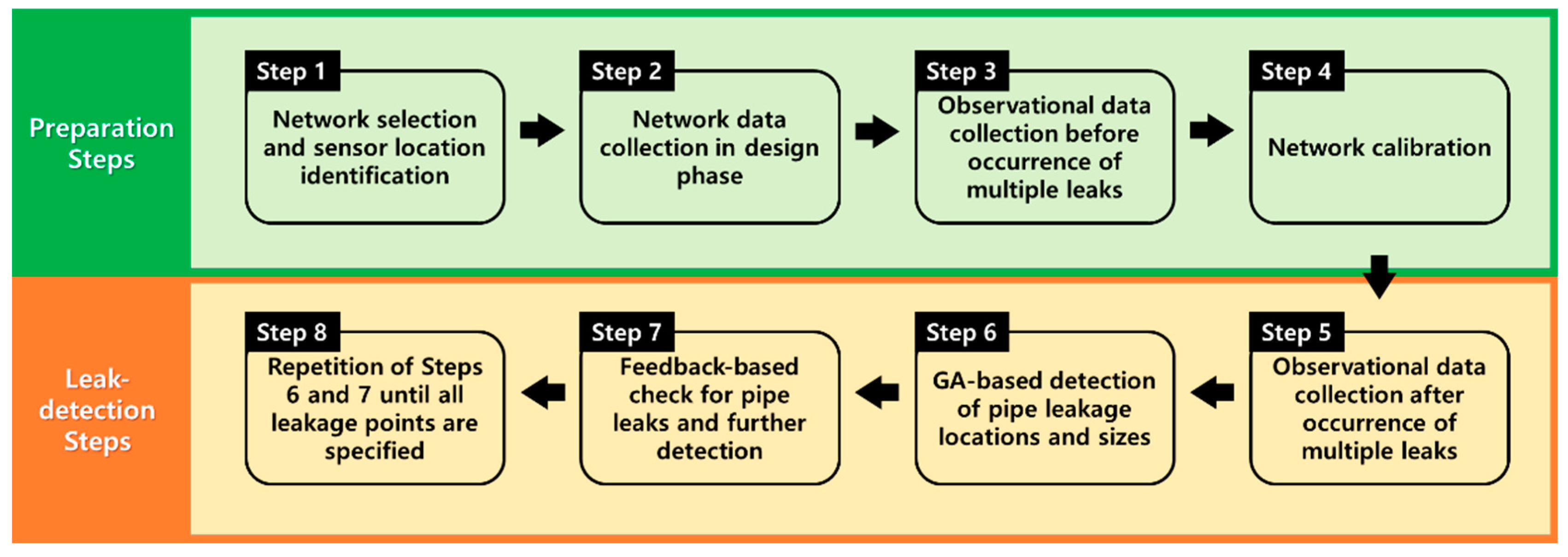
In this study, the proposed multiple-leak detection framework is developed and implemented as a computer model, called LeakFINDER, which is based on MATLAB (MathWorks, Natick, MA, USA) [17] in conjunction with EPANET [18]. EPANET is utilized for the WDN hydraulic analysis, and MATLAB is employed for simulation, such as selection of pipes with potential leaks using an optimization method and simulation of the cooperation between the analysis and fieldwork teams. The developed multiple-leak detection framework consists of eight steps, as shown in Figure 1. The steps are briefly described as follows:

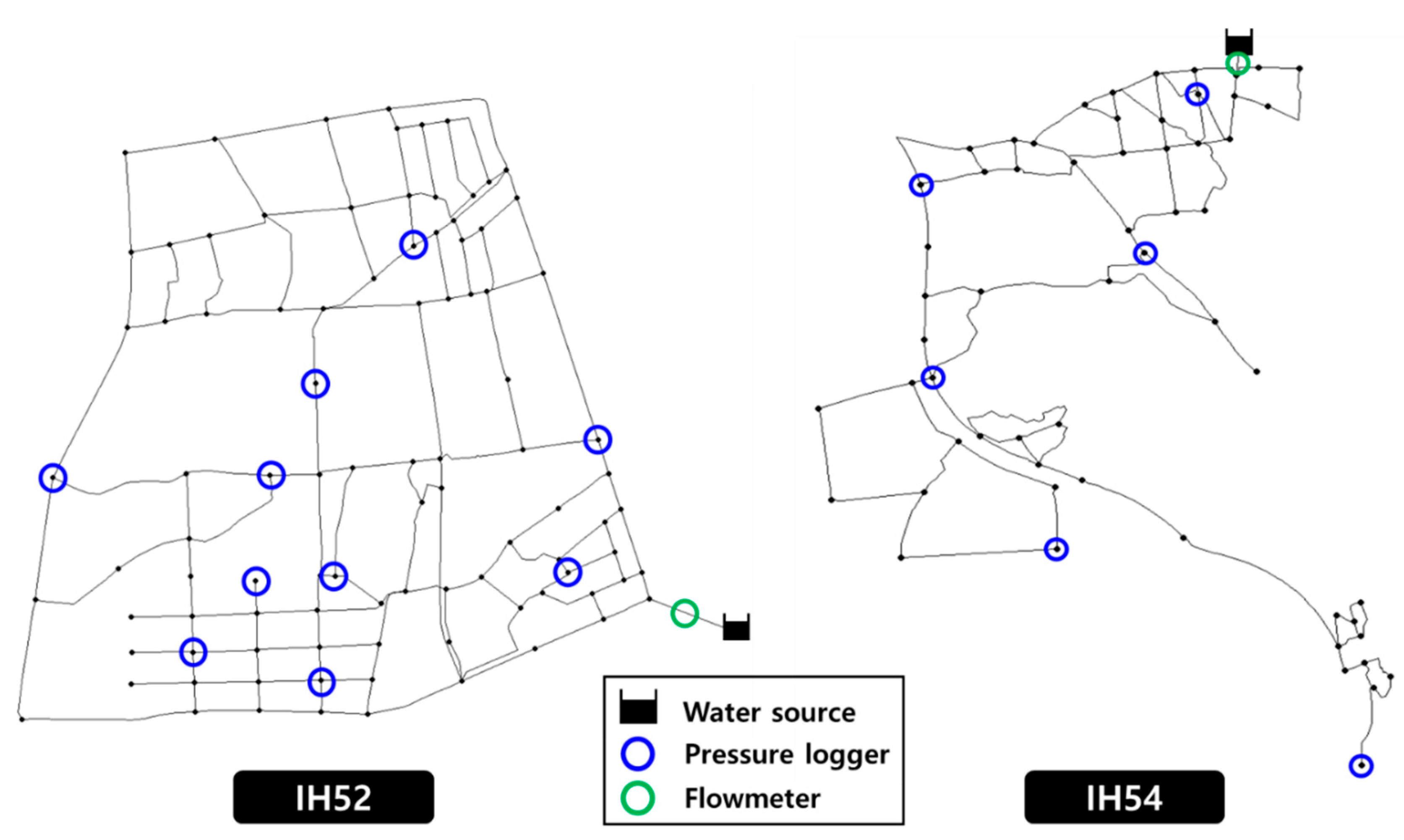
Step 1: The DMA with potential damage due to multiple leaks is selected, and the sensor (e.g., pressure logger and flowmeter) locations are identified.

Step 2: Network information on the selected DMA is collected for hydraulic simulation.

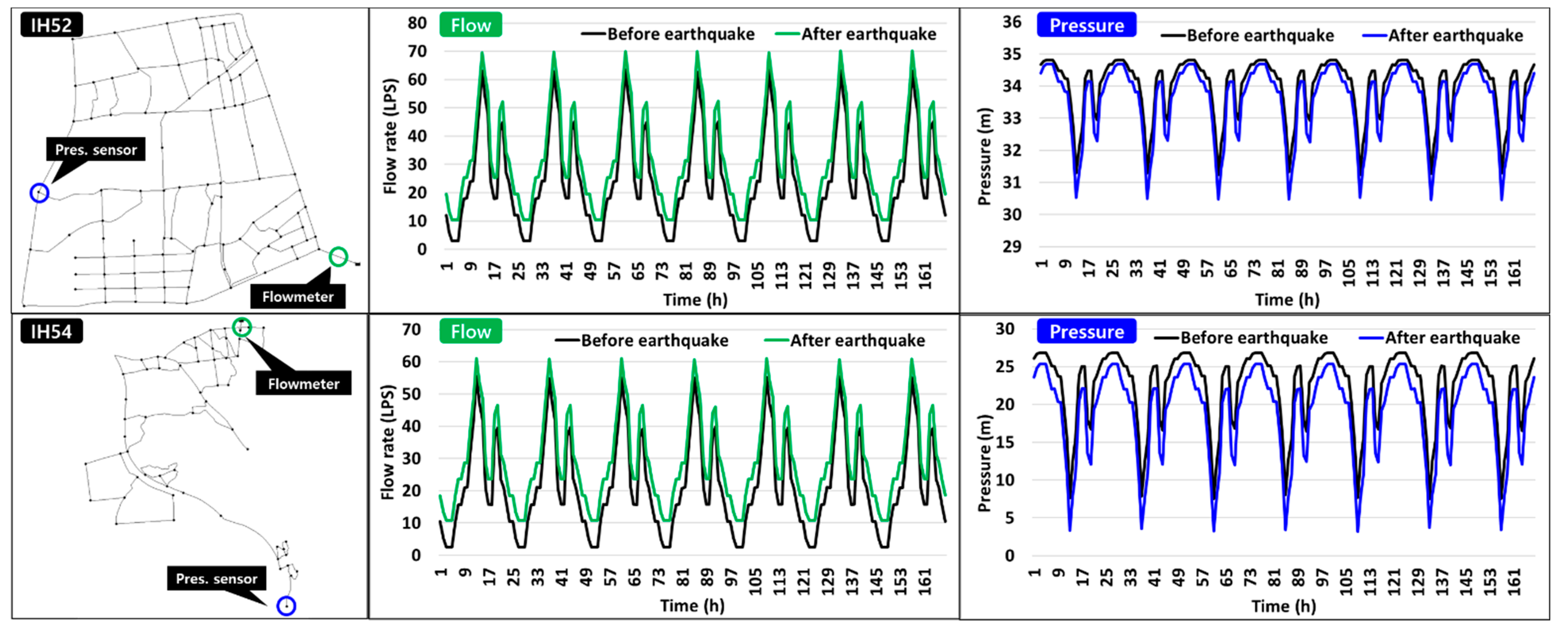
Step 3: Field data (e.g., pressure and flow rate) observed before leak occurrence (caused by an earthquake) are collected.

Step 4: The target network is calibrated based on the observational data collected in Step 3.

Step 5: Observational data (e.g., pressure and flow rate) after leak occurrence (caused by an earthquake) are collected.

Step 6: The analysis team searches for leaking pipes using the network calibrated in Step 4, the post-event field data collected in Step 5, and the developed model (the LeakFINDER analysis module). Information on the identified pipes is supplied to the fieldwork team for field examination.

Step 7: Following field examination by the fieldwork team, the search results are returned to the analysis team for incorporation in a new analysis. If the fieldwork team determines that the previously selected pipes have no leakage, those pipes are excluded from the search pool of the new analysis. If the previously selected pipes are found to have leaks, they are fixed as leaking components but are also excluded from the search pool in subsequent simulations.

Step 8: Steps 6 and 7 are repeated until the analysis team no longer detects pipes with potential leaks. Multiple-leak detection is completed subject to the assumption that all leakage points are specified.

2.2. Multiple-Leak Detection Model (LeakFINDER)

LeakFINDER, the developed multiple-leak detection model, is a computer simulation-based indirect leak-detection model that can yield improved DE by reducing the time and financial costs generated prior to field leak detection. The DE of multiple-leak detection can be improved through real-time cooperation between the analysis and fieldwork teams. The analysis team estimates the pipes with high-leak probabilities and the results are delivered to the fieldwork team for field examination. Subsequently, the fieldwork team returns their field detection results to the analysis team as feedback, and the analysis team conducts reanalysis or redetection based on those field-examination results. The model uses WDN observational hourly data (at 3–5 a.m., nodal pressure and pipe flow rate) as input, and the location of leaking pipes and leakage flow rate are provided as the simulation outputs.

2.2.1. Multiple-Leak Detection

In this study, a GA was used as the optimization method for multiple-leak detection. The GA is an optimization method that was introduced by Holland in 1975 [19] and was developed using the evolution of living organisms and Darwin’s “survival of the fittest” theory as the basic concepts. In this study, hydraulic analysis and optimization were performed in conjunction using the simple GA and EPANET Toolkit embedded in MATLAB. Based on the calibrated network, pipe-leak locations and the leakage volume were estimated through the GA using observational data (nodal pressure and pipe flow rate) after the occurrence of multiple leaks (i.e., after an earthquake). The parameter values for the GA applied in this model are listed in

Table 1. GA parameter values.

Parameter	Value
No. of Population	40
No. of Generation	2500
Crossover rate	0.8
Mutation rate	0.2
Elite count	10%

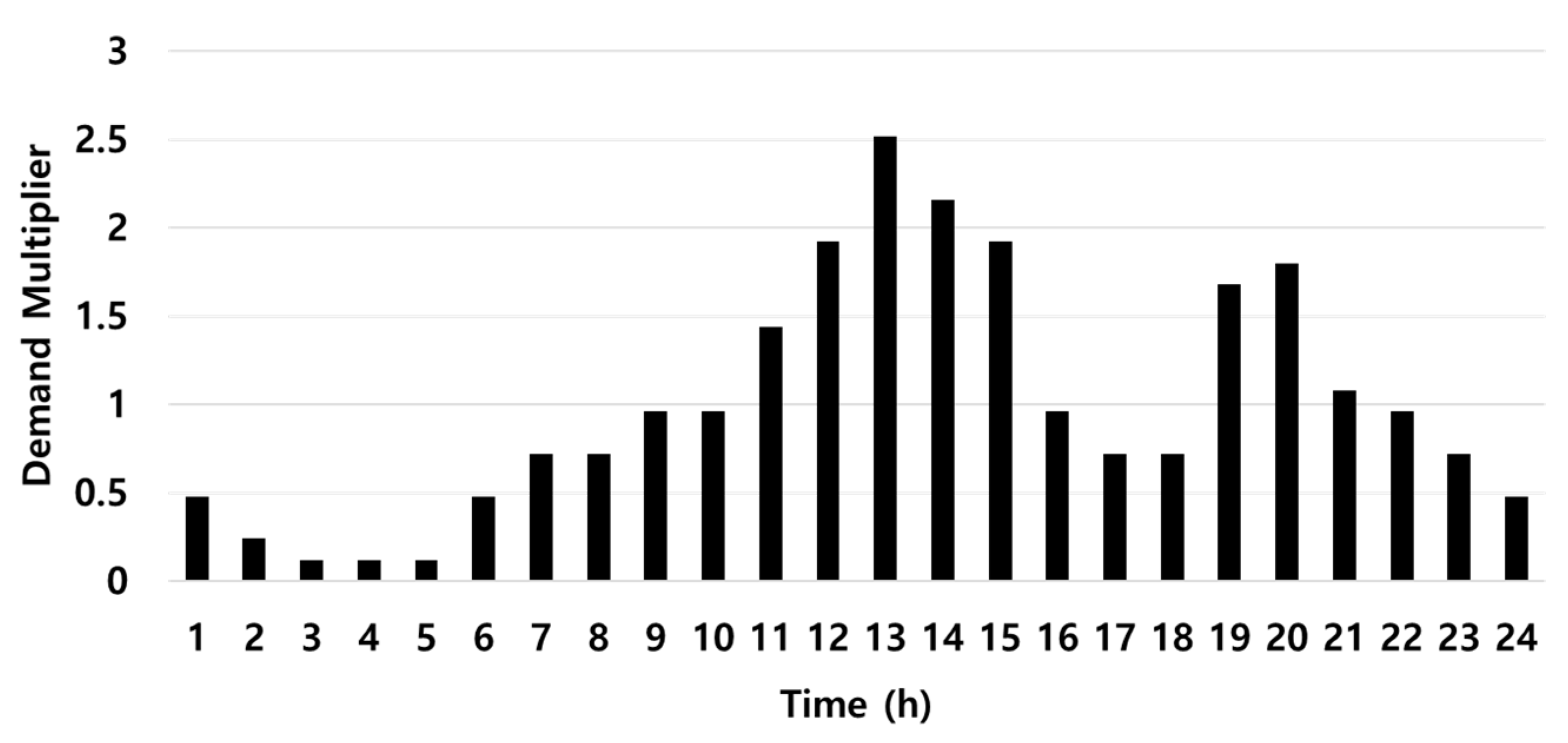
. The three decision variables of the optimization model for multiple-leak detection are as follows: (1) the pipe index of the leaking pipe, (2) the leakage volume from the pipe (determined by the orifice discharge coefficient ($C_d$)), and (3) the total system water consumption (excluding the leaking water). In this study, values measured on-site after the occurrence of multiple leaks were used as the observational data for multiple-leak detection. As a higher leak DE is expected in a low-water-consumption state, nodal pressure and system inflow values recorded during the early morning hours (3–5 a.m.) were used.

The objective function of the optimization model involved minimization of the root-mean-squared error (RMSE) between the observed and simulated pressure values at all sensor locations after the occurrence of multiple leaks, as defined in Equation (1):

$$Minimize:sum\left(RMSE\right)={\displaystyle \sum }_{s=1}^{NS}\sqrt{\frac{{{\displaystyle \sum }}_{t=1}^T{\left(P_{obs,s}^t-P_{sim,s}^t\right)}^2}{T}}$$

(1)

where NS is the number of sensors (pressure loggers), T is the simulation time, and $P_{obs,s}^t$ and $P_{sim,s}^t$ are the observed and simulated pressure values of the s-th sensor at time t, respectively.

2.2.2. Cascade Search for Multiple-Leak Detection

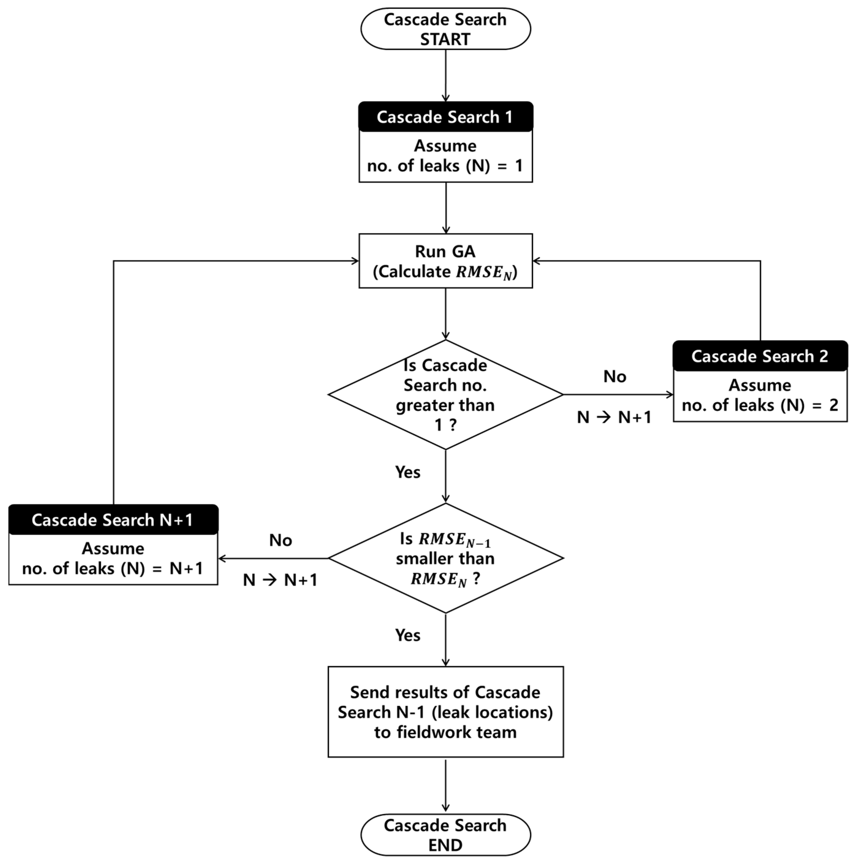
When multiple leaks occur simultaneously in several pipes after an earthquake, it is not possible to determine the number of leaks in the target network, because the underground leaks cannot be visually confirmed. Therefore, in this study, a cascade search method is proposed. In this approach, the possible leaks are searched for sequentially (starting from one leak and increasing the number of potential leaks in each round) to detect the multiple leaks, the number of which is unknown. As shown in Figure 2, for the first search (Cascade Search 1), leak detection is performed assuming that the number of leaks is one. In this instance, the decision variables for leak-detection optimization are $P{I}_1$, $C{d}_1$, and $F_s$, i.e., the leaking-pipe index, the orifice discharge coefficient (i.e., amount of leakage) of this pipe, and the total water flow into the system (excluding leakage), respectively. Upon completion of the leak-detection optimization of Cascade Search 1 (i.e., one leak simulation), two-leak detection optimization is performed (Cascade Search 2). In this instance, the decision variables for leak-detection optimization are expanded to $P{I}_1$, $P{I}_2$, $C{d}_1$, $C{d}_2$, and $F_s$. Note that $F_s$ denotes the water consumption of the entire network (DMA scale) without leaks and thus has a single value regardless of the number of leaking pipes. The proposed cascade search technique continues in this manner, with the number of potential leaks being incremented by one in each round (the number of decision variables is 2N + 1, where N is the number of leaking pipes) until the objective function of the optimization (Equation (1)) no longer improves. When the simulation results are closest to the observed values, the results obtained by the analysis team, that is, the number of leaks and their locations, are delivered to the fieldwork team for field exploration.

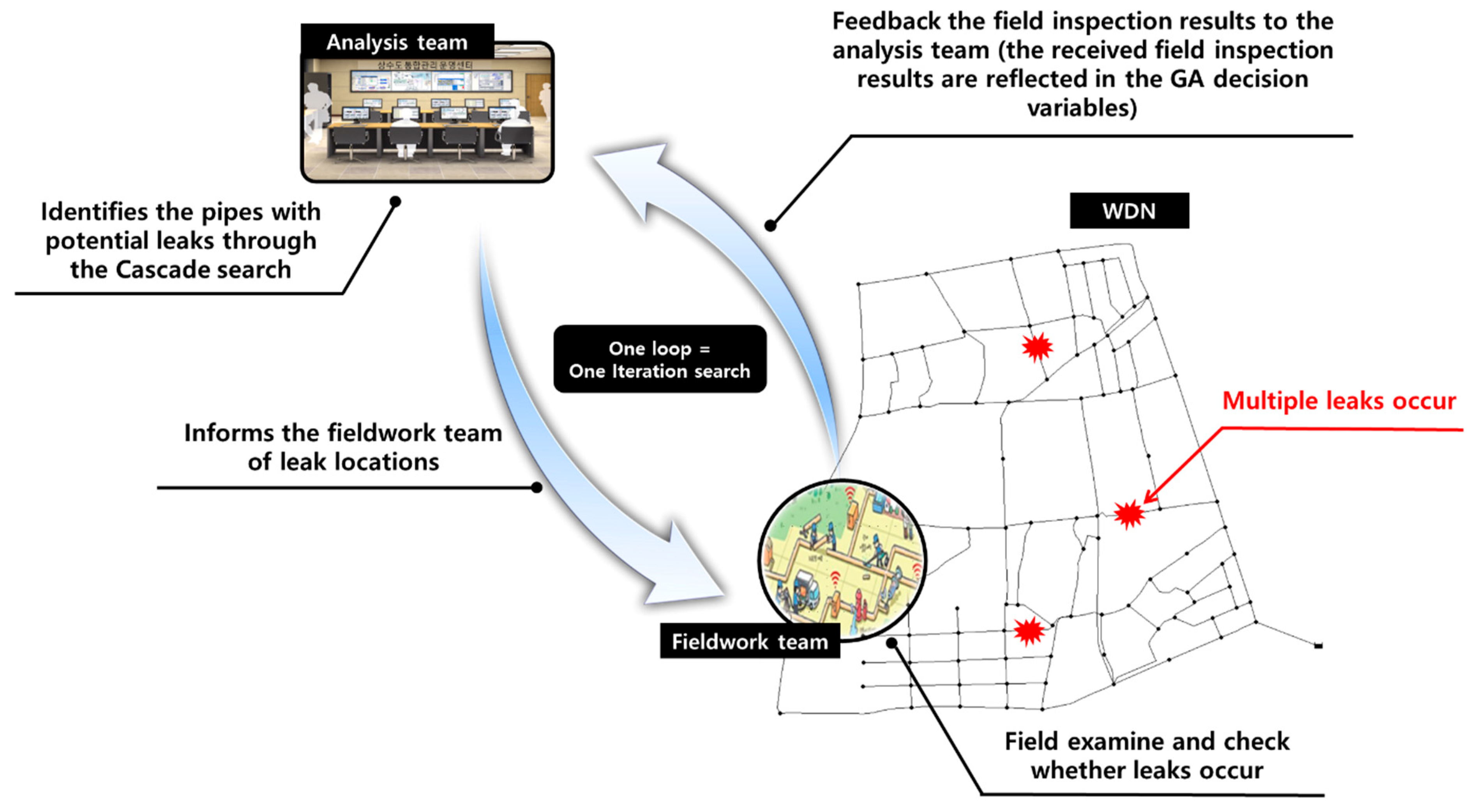
2.2.3. Iteration Searching between Analysis and Fieldwork Teams

In the iteration search stage, the analysis and fieldwork teams cooperate. First, the analysis team identifies the pipes with potential leaks through the cascade search and informs the fieldwork team of these pipe locations for field examination of the potential leaks. The fieldwork team verifies the leakage of the identified pipes on-site. The field-examination results are returned to the analysis team for further simulation, although the need for reanalysis is determined based on the feedback from the fieldwork team. In other words, if the fieldwork team confirms that the identified pipes have no leaks, those pipes are excluded from the optimization search pool in the subsequent simulation by the analysis team. This treatment reduces the optimization search space and improves the optimization efficiency. On the other hand, if the fieldwork team confirms that the selected pipes have leaks, those pipes are fixed as leaking pipes (the locations and leak opening areas of those pipes are reflected in the subsequent analysis); they are also excluded from the optimization search space. Based on the examination results provided by the fieldwork team, the analysis team conducts subsequent simulations (i.e., a cascade search) and delivers new analysis results to the fieldwork team for further field investigation. This iterative searching between the analysis team (running the cascade search) and fieldwork team (performing field examination) is repeated until the analysis team no longer detects pipes with potential leaks (i.e., there is no further improvement in the objective function). The iteration search process for cooperation between the analysis and fieldwork teams is illustrated in Figure 3.

2.3. Leak Detection Efficiency (DE)

Because leak detection requires considerable time and entails substantial expenses, the DE of the developed model is important. In this study, to evaluate the effectiveness of the proposed method, DE was calculated as expressed in Equation (2):

$$DE(\%)=\left(1-\frac{N_s-N_l}{N_p-N_l}\right)\times 100$$

(2)

where $N_s$ is the number of pipes examined by the fieldwork team, $N_l$ is the number of leaking pipes, and $N_p$ is the total number of pipes in the network.

3. Application Network and Data

3.1. Application Network

In this study, two DMA-sized WDNs currently operating in South Korea were selected for application of the proposed model. The two selected networks have different types of pipe layouts, which allowed comparison of the DE values obtained using the developed method for different network layouts. The network layouts are shown in Figure 4. The IH52 network, which is a loop-type network, consists of 95 nodes and 145 pipes, with a base demand of approximately 2160 m³ per day (CMD). The IH54 network, which is a branch-type network, consists of 59 nodes and 85 pipes, with a base demand of approximately 1900 CMD. Figure 5 shows the 24 h water demand pattern applied to the study networks.

3.2. Multiple-Leak Cases

For demonstration of the proposed model, three hypothetical multiple-leakage scenarios were developed for the study networks. In each of the three cases, leaks were assumed to occur at three locations simultaneously (caused by an earthquake) and to have the same leak opening area (5% of the pipe cross-sectional area). Figure 6 shows the multiple-leak locations assumed for each case. As shown in the figure, the following location patterns were purposely implemented for the different cases, to simulate diverse event occurrences: Case 1: leaks distributed evenly throughout the network; Case 2: leaks concentrated in the upstream zone; and Case 3: leaks concentrated in the downstream zone.

Table 2. Leakage information for the application cases.

		IH52 Network		IH54 Network
		Leaking-Pipe Diameter (mm)	Leakage (LPS 1)	Leaking-Pipe Diameter (mm)	Leakage (LPS 1)
Case 1	Leak 1	100	2.61	100	2.88
	Leak 2	80	1.83	100	2.76
	Leak 3	100	3.06	100	2.72
Case 2	Leak 1	80	1.84	80	1.92
	Leak 2	80	1.82	80	1.82
	Leak 3	80	1.83	100	2.75
Case 3	Leak 1	80	1.79	100	2.94
	Leak 2	100	3.22	80	1.71
	Leak 3	80	1.75	80	1.70

¹ LPS: Liter per second (L/s).

summarizes the generated leakage information for the cases considered in this study. Because the leak opening area was assumed to be 5% of the pipe cross-sectional area, the leakage flow varied depending on the leaking-pipe diameter. In addition, pipes with the same diameter exhibited different leakage values depending on the hydrodynamic pressure. Note that the leakage data listed in Table 2 were collected during early morning (3 a.m.), when the water consumption was the lowest.

3.3. Synthetic Field Data Generation

Synthetic field data were generated using the hydraulic analysis model (EPANET) based on the multiple-leak cases mentioned in Section 3.2. The WDN field data essentially consisted of observational data collected using pressure loggers and flowmeters. Therefore, prior to field data generation, the appropriate pressure-logger locations were selected based on a sensitivity analysis. Synthetic data were then collected at the selected locations. During creation of the synthetic data, realistic uncertainty factors were considered to mimic actual network conditions, as detailed in the following subsection.

3.3.1. Optimal Pressure-Logger Placement

Because the efficiency of the data-based leak-detection method is significantly affected by the observation locations and the reliability of the observed values, the appropriate instrument locations must be selected first. In this study, sensitivity analyses were conducted to select the optimal pressure-logger locations in the application network. The analyses were conducted by generating a single leak in each pipe. The pressure at each node was then compared with the leak-free observation to determine the pressure change. As part of the sensitivity analysis, hydraulic analysis was conducted considering various uncertainties likely to occur in the field. The uncertainties included the variations in pipe diameter, roughness coefficient (C_HW), water consumption (i.e., spatial and temporal variation), and leakage rate. To incorporate the uncertainties of these factors into the analysis, sensitivity analyses were conducted by performing random simulations 100 times. The results were then averaged. The sensitivity analysis procedure used for selection of the pressure logger locations was as follows:

• Field data (nodal pressure) prior to leak occurrence (i.e., leak-free condition) were simulated (considering the uncertainties in pipe diameter, C_HW, and water consumption).
• After a single leak was generated in each pipe (considering the leakage flow uncertainty), field data (nodal pressure) were simulated.
• For each single leak generation, 100 random simulations were performed to consider the input uncertainties.
• The sensitivity was analyzed by comparing the data (nodal pressure) collected before and after the occurrence of each single leak. That is, the average difference in nodal pressure (∆P) before and after the occurrence of a leak and the standard deviation (σ) of the nodal pressure after the occurrence of the leak were calculated. The sensitivity of the corresponding node to leaks can be quantified through ∆P, and the fluctuation range of the corresponding data, i.e., the data reliability, can be identified through σ. As ∆P increases, the corresponding node becomes more favorable as an observation location because it responds more sensitively to leaks. In the case of σ, as the value decreases, the corresponding node becomes more preferable as a metering location because its data exhibit less fluctuation and are more reliable.
• The ranking of each node was calculated based on its ∆P and σ values. The nodes with the highest rankings were finally selected as the pressure-logger installation locations.

The pressure-logger locations in the application networks were selected based on the aforementioned procedure. A flowmeter was installed in the main pipe connected to the source for measurement of the network water consumption and leaks. Ten and six pressure loggers (approximately 10% of the total node number) were installed in IH52 and IH54, respectively, as shown in Figure 7.

3.3.2. Field Data Generation

Synthetic field data of the nodal pressure and system flow were obtained from the meters placed in the network (Section 3.3.1). A 30-day hydraulic simulation (extended-period simulation) was conducted using EPANET to generate field data. Various uncertainties were considered during creation of the field data to ensure that these data would emulate the real situations.

The uncertainties considered during creation of the synthetic data were divided into time-fixed and time-varying values. The time-fixed uncertainties were the pipe diameter and C_HW, whereas the time-varying uncertainty was the water demand at nodes. In this instance, both spatial and temporal uncertainties were applied to the water demand calculation. The set ranges of the uncertainty factors employed in this study are listed in

Table 3. Uncertainty ranges considered in the creation of the synthetic field data.

Category	Uncertainty Factor	Range	Distribution Type
Time-fixed uncertainty	Diameter	−5 to 0 mm	Uniform
	Roughness coef. (CHW)	±5	Normal
Time-varying uncertainty	Water demand	±5%	Normal

. Figure 8 illustrates a sample time-series of the synthetic field data of the application networks.

3.4. Network Calibration

For leak detection via hydraulic analysis, the network must be calibrated beforehand. The network calibration was performed using field data collected before the occurrence of leaks and, thus, prior to leak detection. The network calibration involves a process of fine tuning of the computer model close to the actual field condition by determining the pipe diameter and C_HW values. As summarized in

Table 4. Calibration results for the application networks.

Decision Variable	Design Value	Calibrated Value
		IH52	IH54
Diameter (mm)	80	74	76
	100	94	98
	150	146	148
	200	192	200
CHW	110 (IH52) 100 (IH54)	119	97

, the pipes in the application networks were calibrated by dividing them into four groups based on the discrete pipe diameter. For C_HW, a single representative value was calibrated for the entire system.

Observational data (i.e., the nodal pressure) obtained in the leak-free condition (i.e., normal condition) were used for the network calibration. The nodal pressures recorded at peak demand times were used, and the decision variables (four diameter values and one representative C_HW value) were calibrated to minimize the differences between the simulated pressure values of the calibrated network and the pressure values recorded by the pressure loggers. Table 4 lists the calibration results for both application networks.

The network calibration was verified by analyzing the mean-absolute error (MAE) between the field-observed and simulated pressures of the calibrated network for each network. The spatiotemporal average of the MAE for the 10 observation nodes of the IH52 network was found to be 0.005 m, and that for the six observation nodes of the IH54 network was observed to be 0.025 m. These results indicate that the calibrated networks had been similarly replicated for the field situations.

4. Application Results

For each multiple-leak case described in Section 3.2, the proposed approach (i.e., cascade and iteration searching) was applied for multiple-leak detection. LeakFINDER was executed using the calibrated networks and field-observed data. The field survey conducted by the fieldwork team was based on the analysis team’s simulation results, and the field survey results were provided to the analysis team for additional iterative searching. For each case, five independent search simulations (i.e., five independent LeakFINDER runs) were conducted, and the average leak DE was analyzed for comparison. In the following sub-sections, the results of the multiple-leak detections performed for the two application networks are presented and discussed in detail.

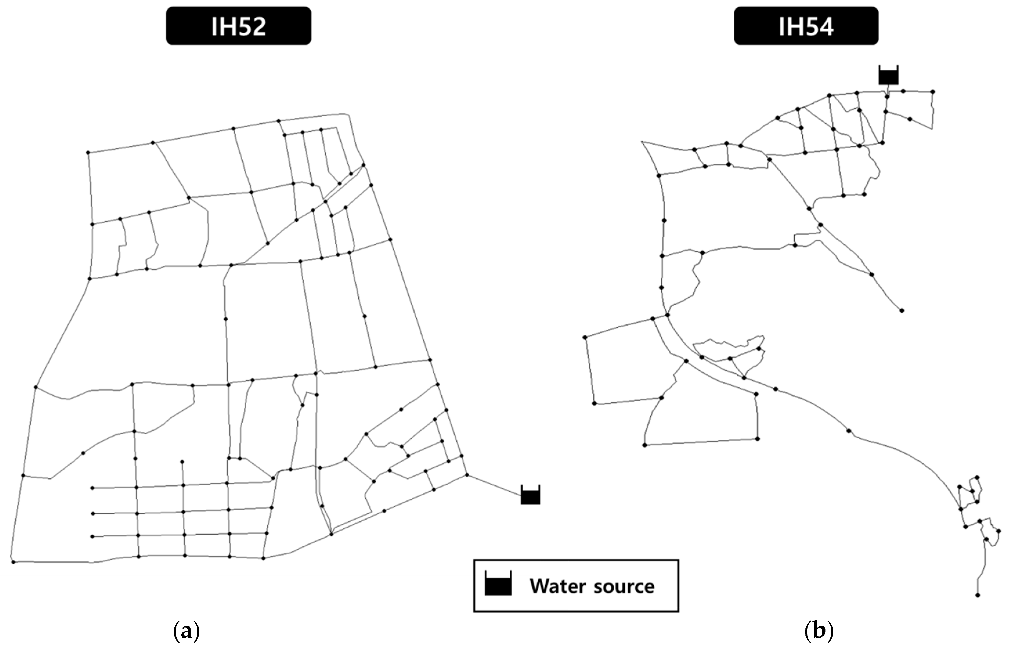
4.1. Multiple-Leak Detection Results (IH52 Network)

The multiple-leak detection patterns and DE of IH52, the loop-type network, were analyzed.

Table 5. Multiple-leak detection efficiency (DE) for each case and run of the IH52 network.

Network	Case	Detection Efficiency (DE) (%)
		Run 1	Run 2	Run 3	Run 4	Run 5	Average
IH52	1	71.8	71.8	71.8	71.8	76.8	72.8
	2	83.1	83.1	88.0	83.1	83.1	84.1
	3	88.0	88.0	88.0	85.9	88.0	87.6

summarizes the DE for each case and each search run (there were three leak cases and five search-runs for each case). As detailed in the table, an average DE of 81.5% was obtained for the three multiple-leak cases, and each run yielded relatively consistent DE values for all cases. Hence, consistent performance was achieved by the proposed multiple-leak detection approach and model. Among the three multiple-leak cases considered for the IH52 network, Case 3 yielded the highest average DE, followed by Cases 2 and 1, in that order.

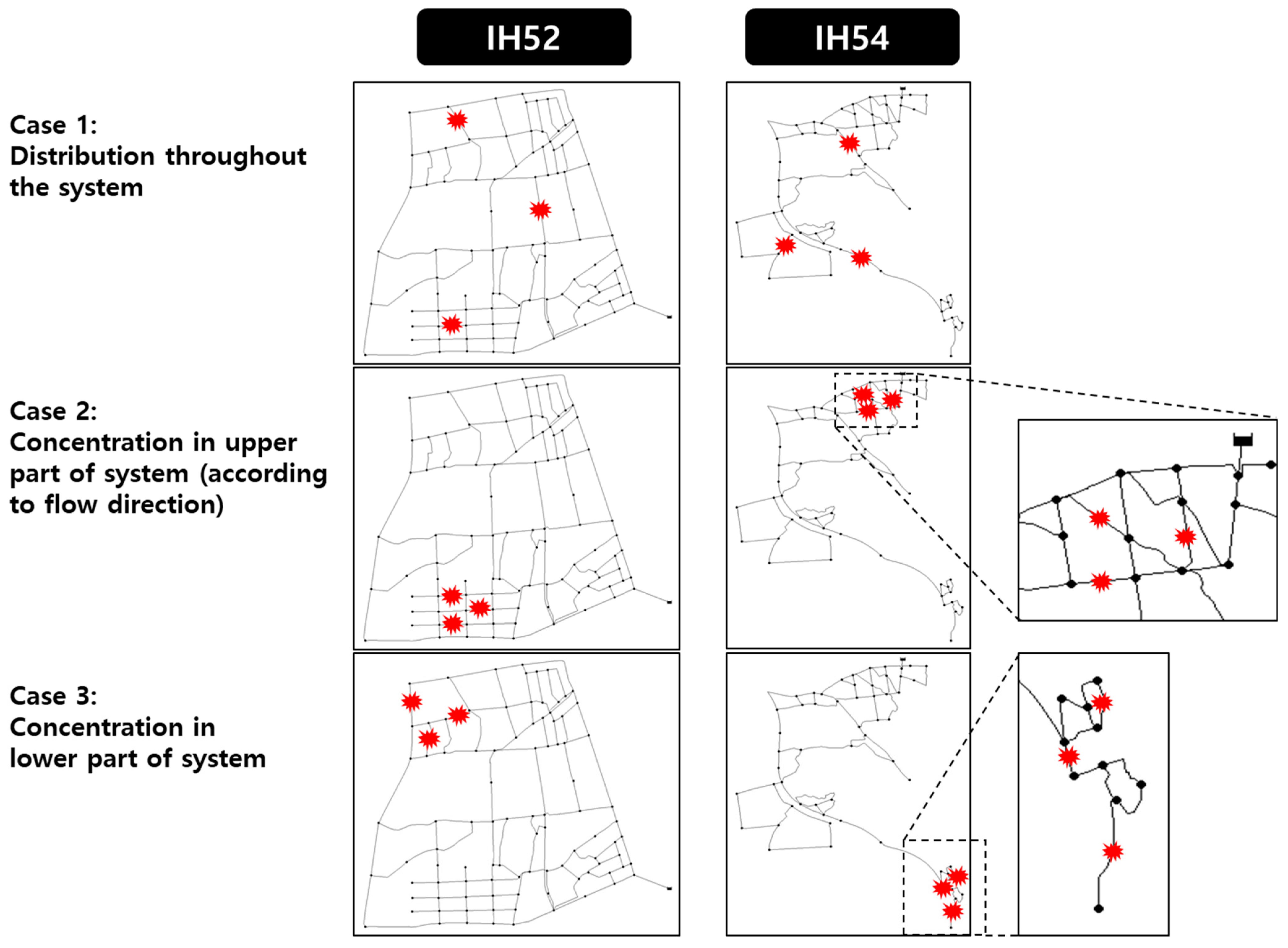
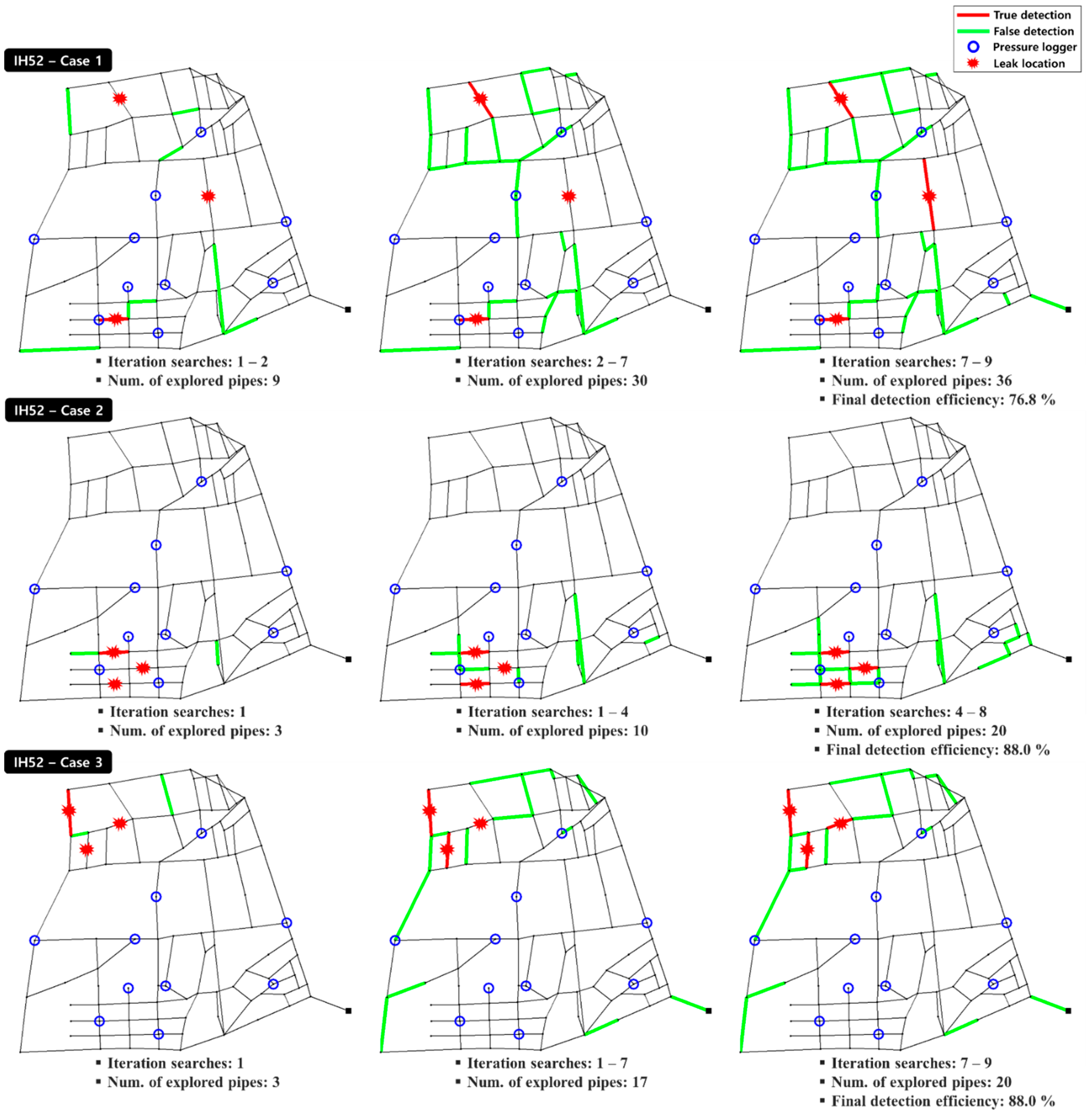
Figure 9 shows the leak-detection sequences of the search run with the highest DE for each case. The search sequences are shown based on the iteration time when the fieldwork team found a new leaking pipe. In the figure, the red lines are the leaking pipes detected in the corresponding iteration (true detection), and the green lines are the false-detection pipes among those examined by the fieldwork team. As shown in Figure 9, the multiple leaks were concentrated in small areas for Cases 2 (upstream zone) and 3 (downstream zone), whereas they were widely spread across the network in Case 1. Thus, a high DE was achieved when multiple leaks occurred in a relatively small area (Cases 2 and 3), but a low DE was obtained when the leaks were widely distributed (Case 1).

Cases 2 and 3, where multiple leaks occurred within a small area, were compared. In Case 3, for which the highest DE was obtained, the multiple leaks were concentrated in the downstream zone of the network. Because the leaks occurred downstream, all nodes located in the flow path to the leakage points were affected from a hydraulic perspective. This induced a pressure drop, especially along the flow paths. This behavior was favorable for leak detection as the changes in nodal pressure were used; hence, a high DE was achieved. In Case 2, where the leaks occurred in the upstream zone of the system, the leak-induced pressure changes were not significant at some observation nodes located in the downstream zone. Hence, a lower DE than that in Case 3 was obtained.

4.2. Multiple-Leak Detection Results (IH54 Network)

The multiple-leak detection results for IH54, the branch-type network, were analyzed.

Table 6. Multiple-leak DE for each case and run of the IH54 network.

Network	Case	DE (%)
		Run 1	Run 2	Run 3	Run 4	Run 5	Average
IH54	1	76.8	79.3	76.8	79.3	79.3	78.3
	2	72.0	68.3	72.0	72.0	72.0	71.3
	3	87.8	87.8	89.0	87.8	87.8	88.0

summarizes the DE for each case and search run. Each run yielded consistent DE values for all study cases, with an average DE of 79.2%. Among the three cases considered for the IH54 network, Case 3 yielded the highest average DE, followed by Cases 1 and 2 in that order. The highest DE was obtained for Case 3 because the multiple leaks were focused in the downstream zone of the network, which simplified the detection, as described in Section 4.1. For Case 2, although the leaks were concentrated in a small area, the lowest average DE (71.3%) was obtained. 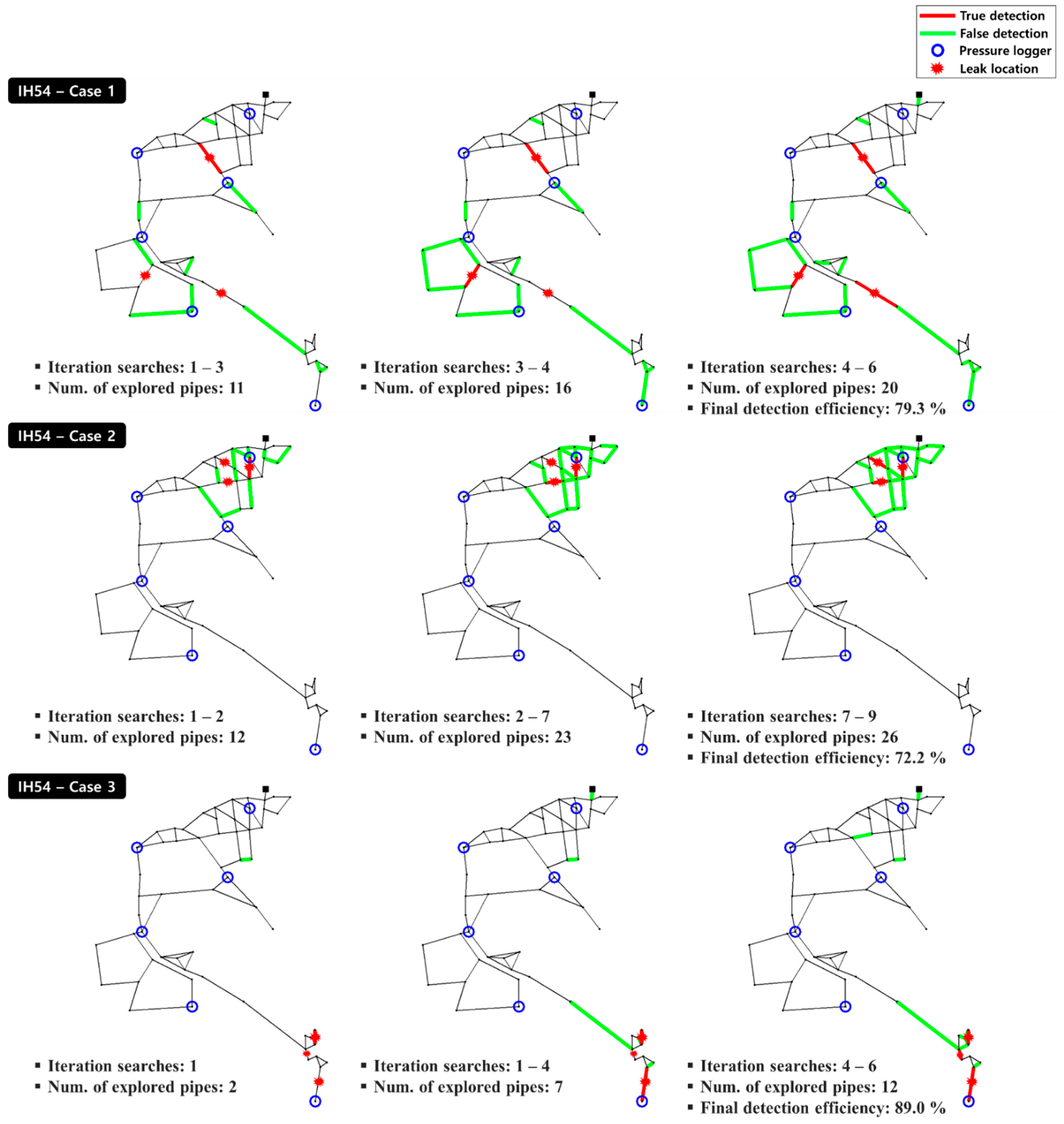Figure 10 shows the multiple-leak search sequences for each case of the IH54 network. For Case 2, multiple leaks occurred in a small area, but they were concentrated in the upstream zone of the network; furthermore, the leaking pipes were located in a complicated loop-type structure. This structure appears to have increased the number of searches for nearby pipes, with many false-detection trials. Conversely, for Case 1, the multiple leaks were dispersed across the network, but the number of nearby pipes to be searched was small owing to the branch-type structure. In addition, the widely distributed sensor locations appear to have contributed to the increase in DE.

4.3. Discussion

The multiple-leak detection results for the two networks with different layouts and three multiple-leak cases in each network show that a high DE was obtained when the leaks were concentrated in a small area in the downstream zone of the system (Case 3). For the IH52 and IH54 networks, average DE values of 81.5% and 79.2%, respectively, were obtained. The average DE for the IH54 network was lower even though it is a branch-type network with a simple structure. This appears to be because the number of installed sensors differed for each network (10 and 6 sensors for IH52 and IH54, respectively) and because notably low DE values were obtained for Case 2 of the IH54 network. The developed model employs hydraulic analysis and an optimization algorithm; thus, leak detection became easier as the volume of field data increased. Accordingly, the IH54 network is considered to be less favorable for the proposed approach because it contained fewer sensors but the same number of applied leaks (three). In addition, it appears that the average DE of the IH54 network was reduced because the DE of Case 2 was considerably reduced owing to the dense loop-type structure that was partially constructed in the upstream zone of the network.

5. Conclusions

In the event of an earthquake, water pipes are highly vulnerable to bursts or leaks. Unlike bursts, which can be visually confirmed because the damage is exposed to the surface layer, leaks are less frequently visible, and discovery of their locations requires considerable time, cost, and manpower. Leak detection methods can be divided into (a) direct observation methods that utilize detection equipment and (b) inference methods based on observational data analysis and computer simulations. The former type is effective for accurately identifying leak locations but generates considerable time and financial costs, whereas the latter type has lower time and financial costs but, also, lower leak detection reliability. In this study, the advantages of both methods were combined for improved leak DE and reliability, and a multiple-leak detection framework based on cooperation between analysis and fieldwork teams was proposed. To that end, a computer model called LeakFINDER was developed, which employs hydraulic simulation and an optimization technique.

The proposed multiple-leak detection method involves a cascade search performed by an analysis team and an iteration search requiring cooperation between the analysis team and the fieldwork team. First, the cascade search is performed to locate multiple leaks. In this process, the number of potential leaks is increased as the search simulation progresses because the actual number of multiple leaks is unknown. Subsequently, the iteration search is performed. In this process, the search efficiency is improved by incorporating the field examination results (i.e., data on true or false detections) in subsequent simulations performed by the analysis team. This approach reduces the cascade search space of the optimization method.

To examine the applicability of the developed model, multiple-leak detection was performed on two DMA-scale networks with different layouts (i.e., loop and branch type), for three formulated cases with different leak locations in each case. The simulation results for the search sequences and the DE were analyzed. The proposed method exhibited consistent performance regardless of the layouts and leak locations of the application networks, and the average DE was 80.4% (ranging from 70 to 90%). These results indicate that the proposed model could identify the locations of all three leaks occurring in the networks by exploring approximately 20% of the pipes in those networks.

In this study, leak detection was simulated by placing virtual sensors and collecting synthetic field data. However, the proposed multiple-leak detection method is expected to improve the efficiency of real-world leak detection (e.g., the required cost, manpower, and time) because it combines the benefits of both direct observation and inference-based methods. In future studies, the developed model will be further improved to achieve higher DE for multiple leaks that are extensively distributed in a network, and simulations will be performed using real-world field data collected from historical seismic events. In addition, sensitivity analyses of various factors that may affect DE (e.g., the number and locations of sensors, the number of leaks, the leakage volume, and measurement errors) will be conducted to improve the performance of the model and widen its field applicability.