Artificial Neural Networks to Forecast Failures in Water Supply Pipes

Abstract

The water supply networks of many countries are experiencing a drastic increase in the number of pipe failures. To reverse this tendency, it is essential to optimise the replacement plans of pipes. For this reason, companies demand pioneering techniques to predict which pipes are more prone to fail. In this study, an Artificial Neural Network (ANN) is designed to classify pipes according to their predisposition to fail based on physical and operational input variables. In addition, the usefulness and effectiveness of two sampling methods, under-sampling and over-sampling, are analysed. The implementation of the model is done using the open-source software Weka, which is specialised in machine-learning algorithms. The system is tested with a database from a real water network in Spain, obtaining high-accurate results. It is verified that the balance of the training set is imperative to increase the predictions’ accurateness. Furthermore, under-sampling prioritises true positive rates, whereas over-sampling makes the system learn to predict failures and non-failures with the same precision.

1. Introduction

The access to drinking water is recognised as an essential human right by the United Nations General Assembly. Management companies of water supply networks are responsible for maintaining the quality of this service. However, for several reasons, these infrastructures have not been maintained over the years on a sustainable basis. In fact, companies from many countries have prioritised short-term repairs instead of rehabilitation actions, which has caused a decrease in the service quality [1]. These rehabilitation activities incur in high maintenance costs. Moreover, water supply networks comprise of a vast extension of pipes, and unexpected pipe failures happen more often than they should. Thus, in order to guarantee the long-term sustainability of the network, an efficient maintenance strategy to target the replacement of the most critical pipes is essential.

To properly manage a water supply company, it is necessary to know in advance the problems and failures that will occur in its components. Intelligent predictive systems are models and algorithms that provide valuable information about the future performance of a system, serving as support for decision-making. In a recent study [2], researchers compare the performances of statistical models predicting failure rates in groups of pipes and machine-learning algorithms forecasting individual pipe failure rates. This work includes some of the most popular statistical models, as linear regression, Poisson regression and Evolutionary Polynomial Regression (EPR). As machine-learning techniques, they use Gradient Boost Trees, Bayesian Belief Networks, Support Vector Machines (SVMs) and Artificial Neural Networks (ANNs). In the study, the authors apply each method separately to pipes made from asbestos cement and PVC. Finally, they conclude that Poisson regression outperforms the two other models according to R² and RSME. Regarding machine-learning models, they do not face the imbalance problem, which is inherent to this type of data, where most pipes do not fail compared to a small percentage that do. Consequently, correctly predicted pipe failure rates are substantially low.

ANNs have shown to be successful in many problems, and they have also been applied as regressive systems in this field to predict the time to failure or the failure rate of pipes [3,4,5,6,7]. In [5], authors employ different ANNs with only one hidden layer to predict pipes’ time to failure. As input variables they use pipe diameter, section length, number of previous failures (NOPF) and protection method, discovering that NOPF is the most influential variable. Moreover, the protection method is shown to significantly increase the time to failure, specifically the cathodic protection for iron pipes. In [7], authors use five input variables (pipe age, diameter, depth, length and average hydraulic pressure) to estimate the failure rates of asbestos cement pipes. As data-driven models, they use ANNs and neuro-fuzzy systems, discovering that ANNs achieve more realistic results. A sensitivity analysis shows that pipe break rates rise as pipe diameter and depth decrease and pressure, age and length increase.

There are also studies that use ANNs to classify the different types of failures that can occur in sewer pipes. Deep convolutional neural networks are used in [8] to detect and classify defects from CCTV (Closed Circuit Television) inspections. Firstly, images are classified into defects/non-defects, achieving accuracies of around 83.2%, and then specific failures are identified. In [9], an automated heuristic approach is employed to find the best ANN configuration considering one hidden layer and up to 50 neurons. Pipe diameter, length, age, depth and slope are the factors used to predict the risk of failure of sewer pipes. In this study, ANNs demonstrate to be superior to SVM, but they also present higher variability. Therefore, they are advised to companies that are less conservative when taking decisions.

In our study, an ANN is designed to forecast pipe failures in water supply networks. Instead of predicting continuous outputs for an aggregation of pipes, our model individually classifies pipes into failure/non-failure using several factors related to the design and operation of the network.

The main contributions of this work are presented as follows:

• The accuracy of ANNs as classification systems to predict pipe failures in water supply networks is evaluated and, in particular, the use of a specific machine-learning software named Weka.
• The effectiveness of two sampling methods, under-sampling and over-sampling, are compared for the first time in this type of problem.
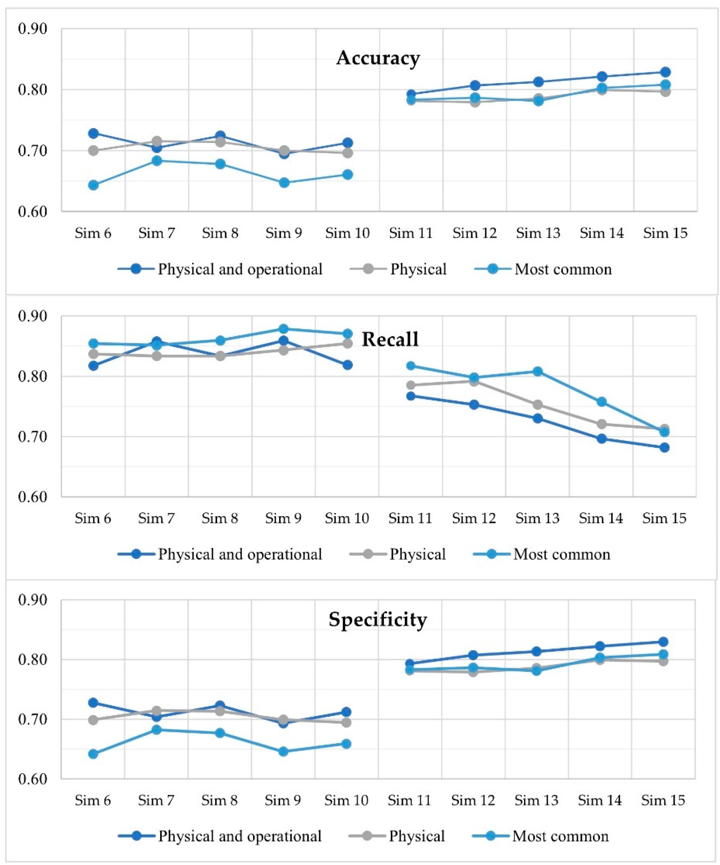
• The influence of physical and operational variables is also tested and discussed.

The paper is organised in four sections, including this introduction (Section 1). Section 2 describes the methodology and the quality metrics used to analyse the results. Then, Section 3 includes the implementation, results and analysis of a real case study. Finally, the conclusions are presented in Section 4.

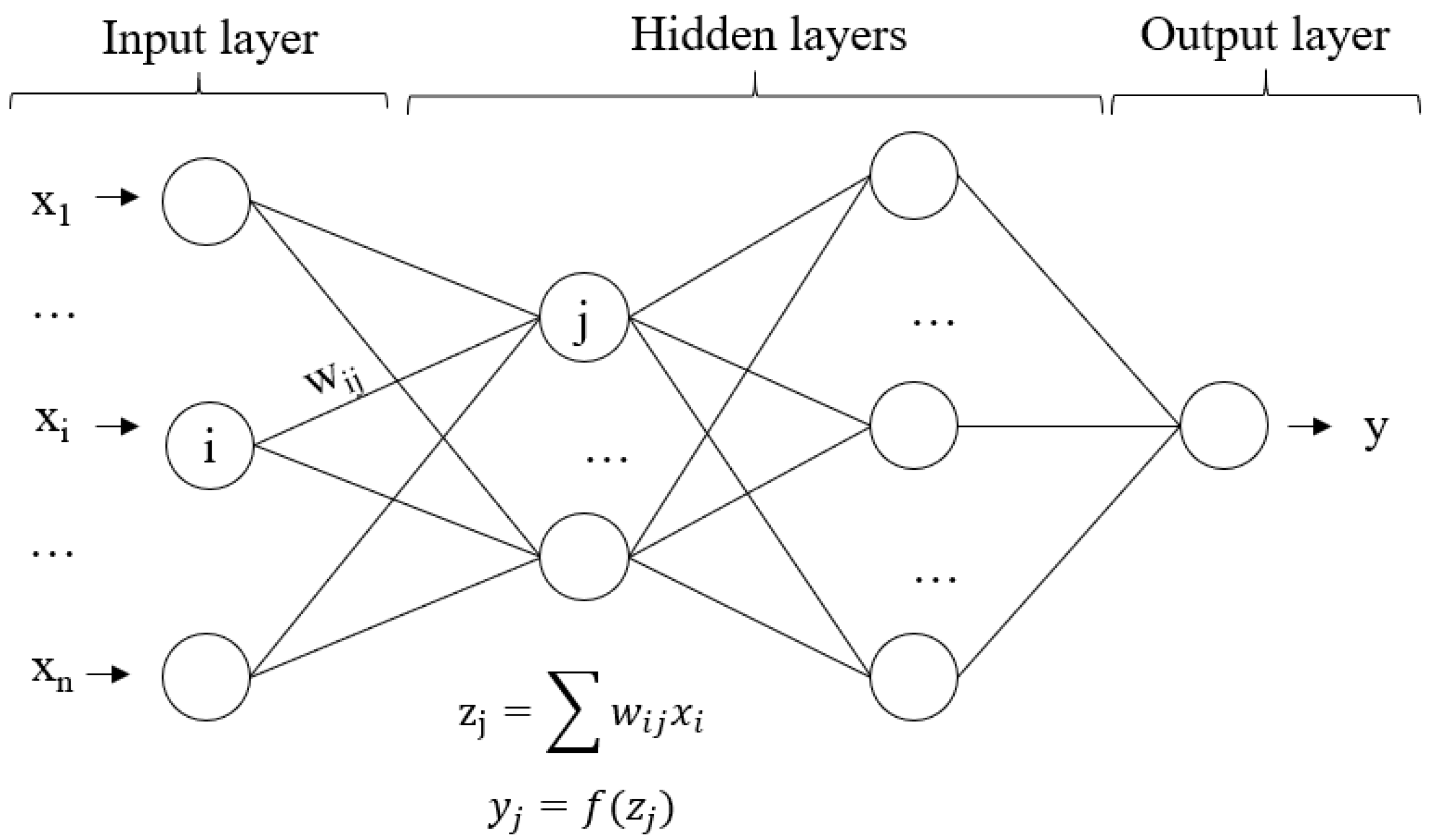
2. Methodology: Artificial Neural Networks

ANNs are systems that emulate the human brain functioning. Neurons are represented by nodes and nerve impulses by the weighted sum of the input values of each node. Although they were first introduced by McCulloch and Pitts in 1943 [10], they did not become relevant until the 21st century because they require huge amount of data to be trained, and the existing computation was not able to support their structures [11].

In ANNs, the interconnected nodes are organised in layers: (1) the input layer receives the information (input variables) and is usually referred to as layer 0; (2) the intermediate or hidden layers process the information; and (3) the output layer generates the output variable (the class in the case of classification problems). Multilayer networks, those with more than one hidden layer, have gained popularity due to the emergence of backpropagation training mechanisms [12]. Figure 1 shows the main component of a multilayer network with two hidden layers.

In each layer, it is firstly calculated the weighted sum of the outputs of the previous layer (z_j). Then, activation functions f(z_j) convert the inputs of each node into its output. The most common activation function is the sigmoid (Equation (1)), but there are other options, such as the rectified linear unit (ReLU) and the hyperbolic tangent. The learning of an ANN is the adjustment of its parameters (w_ij), while its structure does not usually vary [13].

f(z) = 1/(1 + e^−z)

(1)

In this study, the designed ANN has sigmoid activation functions at each node and a different number of hidden layers.

Since the aim of the ANN is to classify, we use the confusion matrix as the quality metric to measure the precision of the results; more specifically, the accuracy, the recall, the specificity and the precision (Equations (2)–(5)), which depend on the number of True-Positives (TP), True-Negatives (TN), False-Positives (FP) and False-Negatives (FN) predictions. These figures rely on the number of samples that are correctly or incorrectly classified from each class.

Accuracy = (TP + TN)/(TP + TN + FP + FN)

(2)

Recall = TP/(TP + FN)

(3)

Specificity = TN/(TN + FP)

(4)

Precision = TP/(TP + FP)

(5)

Furthermore, we use the Mean True Rates (MTR) to identify the best configuration of parameters, as this metric considers both the recall or TP rate and the specificity or TN rate (Equation (6)).

MTR = 1/2·[TP/(TP + FN) + TN/(TN + FP)]

(6)

All the aforementioned metrics move in a range between 0 and 1. Moreover, the closer to 1, the better the performance of the classifier. It is especially important to analyse all the metrics if the dataset is unbalanced to get an overview of the quality of the predictions.

3. Implementation and Results

This section is divided in three subsections: (1) firstly, data from a real case study is presented; (2) secondly, the software used to implement the machine-learning system is introduced as well as some aspects of the training-test process; and (3) finally, the results are summarised by means of graphics and tables.

3.1. Case Study: The Water Supply Network of Seville (Spain)

Data from a real water network are used to evaluate the designed ANN performance. The public company that manages the water network of Seville (EMASESA) has provided a 7-year historical failure database, including various factors that can influence the failure of pipes. Concretely, material, pipe diameter, age, length, connections per kilometre, network type, pressure fluctuation and number of previous failures are used as factors.

Table 1. Data description.

Variable	Type	Min	Max	Mean	Std
MAT—Material	Categorical	CI, DI, AC, CON and PE
DIA—Diameter (mm)	Numerical	20	1700	152.32	142.09
AGE—Age (years)	Numerical	0	118	24.91	17.15
LEN—Length of the segment (m)	Numerical	0.5	4295	42.86	79.28
CON—Connections per km	Numerical	0	11.44	0.05	0.22
N_type—Network type	Categorical	Transport and Secondary
∆PRE—Pressure fluctuation (m)	Numerical	0	27.24	2.88	2.16
NOPF—Number of Previous Failures	Numerical	0	10	0.04	0.28

shows some of the main characteristics of these variables. For numerical variables, the range, mean and standard deviation are presented, and for categorical variables, the categories are shown. These data are an updated version of those used in two previous studies carried out by the authors [14,15], so interested readers are encouraged to consult the cited articles for more information. Despite having used data from the same water network, some new aggregations and filters are applied. For example, instances from pipes whose material represents less than 1% of the total network length have not been considered, and the different polyethylene pipes have been merged. Consequently, the material variable (MAT) can take five different categories: Cast Iron (CI), Ductile Iron (DI), Asbestos Cement (AC), Concrete (CON) and Polyethylene (PE), and the total network length is 3840 km. Moreover, the output variable ‘y’ in this study represents whether or not a pipe fails in 2018, and the variable NOPF contain the failures between 2012 and 2017.

It is well known that ANNs performance improves when the values of the variables move in a range of (0, 1). On the one hand, numerical input variables are normalised following Equation (7). On the other hand, categorical variables are coded using dummies, which means that one binary variable is generated for each category.

x_i = (x_i − x_min)/(x_max − x_min)

(7)

3.2. Implementation

The proposed ANN is implemented in Weka, an open-source software developed by a research group from the Waikato University (New Zealand) that offers standard machine-learning algorithms [16]. The software includes numerous data processing techniques, as well as a wide range of algorithms. Despite being a very powerful software, it has some limitations. Firstly, it requires a very specific data structure, so another software or programming language is generally needed to previously adapt the dataset to Weka specifications. In our case, Python 3.7. is used to read the dataset and pre-process the variables. Secondly, the dimension of the datasets the software can work with is limited, and the runtimes are generally higher than using conventional programming languages. Consequently, this software is recommended to work with small or medium-sized datasets and when the objective is to quickly experiment with different algorithms and data processing techniques.

The imbalance in databases is a common problem for predictive classification systems. After reviewing several scientific studies that use machine-learning techniques to improve the management of water supply networks, in [17], it is recommended to use sampling methods to train classifiers. However, this would not be necessary to train regression models. Several methods are reported in the literature to address this issue. Among them, there are two that stand out: under-sampling and over-sampling (Figure 2). Under-sampling consists in randomly removing samples of the majority class, whereas over-sampling is the generation of synthetic samples of the minority class. Both techniques balance the classes of the training set, seeking to improve the learning capacity of the algorithm. In general, mathematicians prefer under-sampling because the use of over-sampling implies the generation of artificial instances and, consequently, it is defended that the entire database becomes unreal. Nevertheless, this technique is supported in this paper as long as the test set is not altered.

The output variable of our database is totally unbalanced, having 619 failures in 2018 out of 89,595 pipe sections. This is a common fact in water supply databases where the number of pipe failures is very small compared to the entire network. For this reason, the study compares the use of the above-mentioned sampling techniques to train the ANN. Under-sampling is randomly applied, while the generation of synthetic instances in over-sampling is done using a 5-nearest neighbours’ approach.

3.3. Results and Discussion

Table 2. Results—Physical and operational variables.

Sim.	HL	Sampling Method	Acc.	Rec.	Spec.	Prec.	Runtime (s)
1	1	None	0.993	0.000	1.000	0.000	110.5
2	5	None	0.993	0.002	1.000	0.111	223.5
3	10	None	0.993	0.002	1.000	0.100	385.0
4	50	None	0.993	0.005	1.000	0.250	1885.0
5	100	None	0.993	0.005	1.000	0.176	3716.1
6	1	Under-sampling	0.728	0.817	0.728	0.020	2.0
7	5	Under-sampling	0.705	0.858	0.704	0.020	3.6
8	10	Under-sampling	0.724	0.834	0.723	0.021	6.4
9	50	Under-sampling	0.694	0.859	0.693	0.019	29.3
10	100	Under-sampling	0.691	0.864	0.690	0.019	58.8
11	1	Over-sampling	0.793	0.767	0.793	0.025	263.9
12	5	Over-sampling	0.807	0.753	0.807	0.026	502.1
13	10	Over-sampling	0.813	0.730	0.813	0.026	883.6
14	50	Over-sampling	0.822	0.696	0.822	0.027	4154.3
15	100	Over-sampling	0.828	0.682	0.829	0.027	8416.1

shows the results of a batch of simulations whose differences are the number of hidden layers (HL) of the ANN and the sampling method. All values are the mean of the obtained ones for the test set in a 5-fold cross-validation process, that is, the original data is iteratively divided into 80% to train the ANN and 20% to test it. Moreover, the runtimes are included to compare, in general terms, the applicability of the different configurations.

As can be seen in Table 2, the use of some sampling method is crucial to obtain suitable results. In fact, simulations 1 to 5 achieve poor results since the failure prediction rate (recall) is near to 0 in all cases.

Among the metrics, the low precision values are remarkable. To explain it, we focus on simulation 6, whose dataset, as in all other simulations, is unbalanced (presented results are for the test set). On the one hand, 72.8% of pipes are well-predicted in this simulation, and of all failures recorded in 2018, 81.7% are correctly predicted as well as 72.8% of real non-failures. On the other hand, of all the failures predicted by the system, only 2% are pipes which really failed (precision of 0.020). This suggests that if the system informs that 100 pipes will fail, only 2 are real failures. This happens due to the unbalanced nature of the data, which makes it necessary to inspect or replace many pipes to avoid only a few failures. Even so, the use of this technique is beneficial for companies, since unexpected pipe failures generate costs much higher than replacement tasks planned in advanced. Finally, runtimes increase as the number of HL grows, and especially in the case of over-sampling, because the training of the algorithm is done with a considerably larger dataset. Simulations have been carried out on a PC with 3 GHz, an Intel Core i5 processor and 16.0 GB of RAM.

ANNs do not allow us to easily interpret the impact or influence of the different variables involved in the predictions. Nonetheless, this is a relevant aspect in this field, where companies and experts demand detailed information about the variables’ importance to focus their effort in correctly registering them. For this reason, we have opted for analysing the predictive capabilities of ANNs using two extra subgroups of input variables.

Table 3. Input variables included in each set.

Input Variables
Physical and operational	MAT, DIA, AGE, LEN, CON, N_type, ∆PRE and NOPF
Physical	MAT, DIA, AGE, LEN, CON and N_type
Most common	DIA, AGE, LEN and NOPF

shows the variables that constitute each group, the first being the original one (presented in Table 1).

The objective is to assess the advantages and disadvantages of including certain variables. Moreover, the different variables’ sets allow us to study the usefulness of operational variables as pressure fluctuation and previous failures, whose recording is more expensive to companies. The first group corresponds to all available variables (results from Table 2), mixing both physical and operational; the second group only contains physical variables; and the last group includes only four variables, which are the most common according to the scientific literature [14]. Contrary to what one might expect, the material is not included in the most common variables. This is because many studies apply machine-learning techniques to single material pipes, or to pipes of different materials independently. Consequently, in these studies, material is not employed as an input variable.

Figure 3 shows the accuracies, recalls and specificities of simulations 6 to 15 for the different variables’ groups. The first five simulations have not been included because they achieve poor-quality results in every case (as can be seen in the case of physical and operational variables in Table 2). Furthermore, due to the significant differences between precision and the other metrics, it has also been excluded from the graphs. The figure is intended to independently show the trend of the metrics, in order to compare the differences between under-sampling and over-sampling and the ANN configuration.

Results suggest that training an ANN with a balanced dataset (1:1) through under-sampling implies that the system will not properly learn how to distinguish patterns of the majority class (in this case, the non-failure), while the minority class (the failure) is detected with high precision. This can be appreciated in simulations 6–10, where the recalls are higher than the specificities. This makes sense since, when using under-sampling, many instances are removed, causing this lack of learning ability. On the contrary, the accuracies and recalls of simulations 10–15 have similar values, which means that over-sampling (1:1) allows the system to distinguish both classes with the same importance. Using physical or the most common variables, over-sampling reaches better results, which is not so clear when all variables (physical and operational) are used.

Accuracies and specificities have, in all cases, analogous values because the test set is unbalanced and, therefore, the non-failure rate is almost identical to the total percentage of correct classifications.

Regarding the input variables, it is observed that using only the most common variables, the recalls are generally higher, which means that the variables’ diameter, age, length and previous failures embrace enough relationships with the failure of pipes.

Given the size of our dataset, 89,595 instances with 619 pipe failures, and attending to the mean between recall and specificity, the best ANN configuration for every group of variables corresponds to five hidden layers (simulations 7 and 12), although results are quite similar when the number of hidden layers is 10. By contrast, they get worse for 50 and 100 HL. This is because the more hidden the layers, the more parameters need to be estimated and, therefore, the more data are required.

Table 4. Mean between recalls and specificities for the best ANN configuration.

Input Variables	Under-Sampling	Over-Sampling
Physical and operational	0.781	0.780
Physical	0.775	0.785
Most common	0.768	0.800

presents the mean between recalls and specificities attained using five hidden layers for each combination of input variables and sampling technique.

Superior results are reached for over-sampling and, specifically, when only the most common variables are used. This informs that it is not so important to have more variables, but to use the appropriate ones. Moreover, it confirms the high influence of diameter, age, length and NOPF on the pipe failures, while other variables, as pressure fluctuation, worsen the predictive abilities of the model. This is obviously related to the quality of the data, as it is very difficult to have pressure data at the exact moment when failures occur.

The best MTR, equal to 0.800, derives from a specificity of 0.783 and a recall of 0.817, and the accuracy of this simulation is 0.783 (5 HL, over-sampling and most common variables). Consequently, the ANN is able to predict 81.7% of pipe failures, having a global accuracy of 78.3%.

Finally, this result attained by our study is compared with those obtained in two previous ones (

Table 5. Comparison between quality metrics obtained in two previous studies and our approach.

Research		Acc.	Rec.	Spec.
[2]	AC pipes	0.999	0.392	0.996
	PVC pipes	0.996	0.429	0.999
[18]		0.830–0.960	0.702–0.808	0.835–0.989
Our study		0.783	0.817	0.783

). In [2], an ANN (among other models) is used to predict pipe failures in a medium-sized Colombian city. The model is independently applied to asbestos cement and PVC pipes. In [18], decision trees learning methods are employed to model water distribution pipe deterioration in a small-sized Austrian city.

It is important to highlight the fact that the metrics cannot be subjectively compared, since they are highly dependent on the size and the quality of the database. In our case, the water network is substantially larger (3840 km) than those of the two other presented studies (1819 and 851 km, respectively), and the imbalance ratio is more accentuated. Nevertheless, these metrics give an idea about the performance of the models, as well as their strengths and weaknesses.

Thanks to the detailed study of the sampling methods, our approach provides superior recalls, which means that the failure is better characterised. However, there is room for improving the accuracies. In [18], they use variables related to valves and house connections achieving great performance, so this seems to be a good option for a future line of research.

4. Conclusions

In this study, an Artificial Neural Network is employed to predict pipe failures in water distribution networks. This is a promising approach to reduce the number of unexpected pipe failures, which cause many problems to management companies and to the whole society because these infrastructures are generally public. Companies are increasing their confidence in data-driven decision-making methods and, especially, machine-learning techniques. This is an important fact given that ANNs are black box systems, so experts in the field need to trust in the capabilities of these models. Tendencies show that they will soon be integrated into the real decision systems of companies.

Several structures of ANN are evaluated by changing the number of hidden layers from 1 to 100. In addition, two sampling-methods, i.e., under-sampling and over-sampling, are assessed to discover which one is more appropriate to the problem under study. The presented methodology is applied to a real case study in Spain using the software Weka. The input variables are material, diameter, age, length, connections per kilometre, network type, pressure fluctuation and number of previous failures. However, the methodology is also implemented for smaller groups of input variables in order to analyse the advantages and disadvantages of including more variables. The output variable is categorical, indicating whether or not a pipe fails in a specific year.

Results demonstrate that the model has an excellent ability to predict failures (recalls up to 80%). In general, a more accurate pipe failure forecast implies the worsening of the no-failure predictions. Therefore, the selection of the model must be done according to the company’s strategy and budget. Furthermore, the necessity of balancing classes in the training set is confirmed in order to obtain accurate predictions, whereas the test set must be untouched for the results to be realistic. The use of four variables (diameter, age, length and previous failures) attains the best performance, demonstrating their influence in the appearance of pipe failure.

ANNs have been widely demonstrated to be accurate predictive systems. As their only disadvantage, these systems are difficult to decipher because they contain many weights. In fact, the more numerous and dense hidden layers, the more weights there are. For this reason, future research lines should target the influence of the variables by means of a good-performance ANN model with different combinations, and then compare the results achieved. This would also help to identify and exclude useless variables.

References

1. ISO/FDIS 24516-1: Guidelines for the Management of Assets of Water Supply and Wastewater Systems; ISO: Geneva, Switzerland, 2016.
2. Giraldo-González, M.M.; Rodríguez, J.P. Comparison of Statistical and Machine Learning Models for Pipe Failure Modeling in Water Distribution Networks. Water 2020, 12, 1153. [Google Scholar] [CrossRef] [Green Version]
3. Almheiri, Z.; Meguid, M.; Zayed, T. Intelligent Approaches for Predicting Failure of Water Mains. J. Pipeline Syst. Eng. Pract. 2020, 11, 1–15. [Google Scholar] [CrossRef]
4. Christodoulou, S.; Deligianni, A. A Neurofuzzy Decision Framework for the Management of Water Distribution Networks. Water Resour. Manag. 2010, 24, 139–156. [Google Scholar] [CrossRef]
5. Sattar, A.M.A.; Ertuğrul, Ö.F.; Gharabaghi, B.; McBean, E.A.; Cao, J. Extreme learning machine model for water network management. Neural Comput. Appl. 2019, 31, 157–169. [Google Scholar] [CrossRef]
6. Shirzad, A.; Tabesh, M.; Farmani, R. A comparison between performance of support vector regression and artificial neural network in prediction of pipe burst rate in water distribution networks. KSCE J. Civ. Eng. 2014, 18, 941–948. [Google Scholar] [CrossRef]
7. Tabesh, M.; Soltani, J.; Farmani, R.; Savic, D. Assessing pipe failure rate and mechanical reliability of water distribution networks using data-driven modeling. J. Hydroinf. 2009, 11, 1–17. [Google Scholar] [CrossRef]
8. Li, D.; Cong, A.; Guo, S. Sewer damage detection from imbalanced CCTV inspection data using deep convolutional neural networks with hierarchical classification. Autom. Constr. 2019, 101, 199–208. [Google Scholar] [CrossRef]
9. Sousa, V.; Matos, J.P.; Matias, N. Evaluation of artificial intelligence tool performance and uncertainty for predicting sewer structural condition. Autom. Constr. 2014, 44, 84–91. [Google Scholar] [CrossRef]
10. McCulloch, W.S.; Pitts, W.H. A logical calculus of the ideas immanent in nervous activity. Bull. Math. Biophys. 1943, 5, 115–133. [Google Scholar] [CrossRef]
11. Géron, A. Hands-On Machine Learning with Scikit-Learn and Tensor Flow; O’Reilly Media, Inc.: Newton, MA, USA, 2017. [Google Scholar]
12. LeCun, Y.; Bengio, Y.; Hinton, G. Deep learning. Nature 2015, 521, 436–444. [Google Scholar] [CrossRef] [PubMed]
13. Sze, V.; Chen, Y.-H.; Yang, T.-J.; Emer, J.S. Efficient Processing of Deep Neural Networks: A Tutorial and Survey. Proc. IEEE 2017, 105, 2295–2329. [Google Scholar] [CrossRef] [Green Version]
14. Robles-Velasco, A.; Cortés, P.; Muñuzuri, J.; Onieva, L. Prediction of pipe failures in water supply networks using logistic regression and support vector classification. Reliab. Eng. Syst. Saf. 2020, 196, 106754. [Google Scholar] [CrossRef]
15. Robles-Velasco, A.; Cortés, P.; Muñuzuri, J.; Barbadilla-Martín, E. Aplicación de la regresión logística para la predicción de roturas de tuberías en redes de abastecimiento de agua. Dir. Organ. 2020, 70, 78–85. [Google Scholar] [CrossRef]
16. Frank, E.; Hall, M.A.; Witten, I.H. Data Mining: Practical Machine Learning Tools and Techniques; Morgan Kaufmann Publishers, Inc.: Amsterdam, The Netherlands, 2016. [Google Scholar]
17. Velasco, A.R.; Muñuzuri, J.; Onieva, L.; Palero, M.R. Trends and applications of machine learning in water supply networks management. J. Ind. Eng. Manag. 2021, 14, 45–54. [Google Scholar] [CrossRef]
18. Winkler, D.; Haltmeier, M.; Kleidorfer, M.; Rauch, W.; Tscheikner-Gratl, F. Pipe failure modelling for water distribution networks using boosted decision trees. Struct. Infrastruct. Eng. 2018, 14, 1402–1411. [Google Scholar] [CrossRef] [Green Version]
Figure 1. Multilayer neural network.
Sustainability 13 08226 g001
Figure 2. Under-sampling and over-sampling techniques. Blue bins represents samples from the majority class, while red bins are samples from the minority class before and after applying each sampling strategy [17].
Sustainability 13 08226 g002
Figure 3. Quality metrics for simulations 6 to 10 (under-sampling) and 11 to 15 (over-sampling) and different numbers of hidden layers.
Sustainability 13 08226 g003