
Optimization Research on Vehicle Routing for Fresh Agricultural Products Based on the Investment of Freshness-Keeping Cost in the Distribution Process


Abstract
:1. Introduction
2. Problem Description
3. Model Formulation
3.1. Parameters and Variables
3.2. Related Cost of the Distribution Process
3.3. Optimize Model Settings
4. Hybrid Ant Colony Optimization (HACO) Design
4.1. Initial Pheromone Settings
- Step 1: Initialize parameters λ and τ0, initialize variable k = 1, and N is the set of optional nodes. Turn to step 2.
- Step 2: T[k] = ϕ, Q(k) = 0, set the distribution center as the center point. Turn to step 3.
- Step 3: If N is an empty set, then turn to step 9, otherwise turn to step 4.
- Step 4: Start from the center point, follow the direction of the smallest values of the heuristic function and search for the next customer i in the set N. Turn to step 5.
- Step 5: Judge whether Q(k) + qi ≤ Q. If customer i satisfies the load capacity constraint of the vehicle, turn to step 6. Otherwise, the vehicle returns to the distribution center and turn to step 8.
- Step 6: Q(k) = Q(k) + qi, center = i, turn to step 7.
- Step 7: Remove customer i from N, put it into T[k], turn to step 3.
- Step 8: k = k + 1, turn to step 2.
- Step 9: Update the initial pheromone and end.
4.2. Heuristic Factor Design
4.3. Transferring and Selecting Rules by Probability
4.4. Pheromone Updating Strategy
4.5. The Pseudo-Code Framework Diagram of Hybrid Ant Colony Optimization
| Algorithm 1 HACO for the Model That Targets the Total Distribution Cost |
| (i) Input: each customer’s coordinates, demand, time window and service time, etc. (ii) Output: optimal path (OP), each component of the minimal total cost (CMTC) and the minimal total cost (MTC). (1) Set N, T[k], NCmax, NC, etc. (2) Construct the initial optimization path and give the initial pheromone according to the A* algorithm. Set K the number of the ants. (3) NC = 1 (4) while NC ≠ NCmax (5) Initialize the ant path, the pheromone of each path. Insert 0 at the first of the ant path. All ants return to the distribution center. (6) for k = 1 : K (7) while N ≠ ϕ (8) Select next customer i according to transferring and selecting rules. Calculate the cargo weight Q(k) if ant n arrive at customer i. (9) if Q(k) ≤ Q (10) Insert customer i to the end of the ant path, update T[k] and delete i from N. (11) else Q(k) > Q (12) Ant k returns to the distribution center, insert 0 to the end of the ant path. Q(k) = 0. (13) end if (14) end while (15) end for (16) Calculate the total cost according to the ant path of each ant, select the optimal path and the minimal total cost for this iteration (MTCn). (17) Update the pheromone of each path according to the optimal path. (18) if MTCn < MTC (19) MTC = MTCn, update OP and CMTC. (20) end if (21) NC=NC + 1 (22) end while (23) return OP, CMTC, MTC |
5. Experimental Design and Result Analysis
5.1. Experimental Data and Parameter Settings
5.2. Validity Analysis of HACO
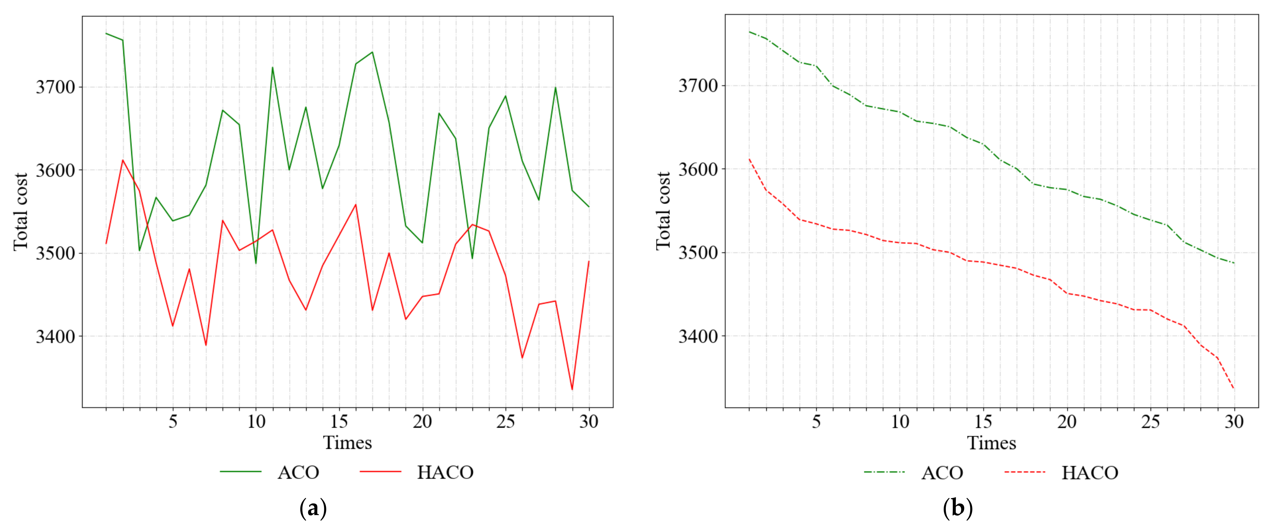
5.2.1. Comparison of Solution Results
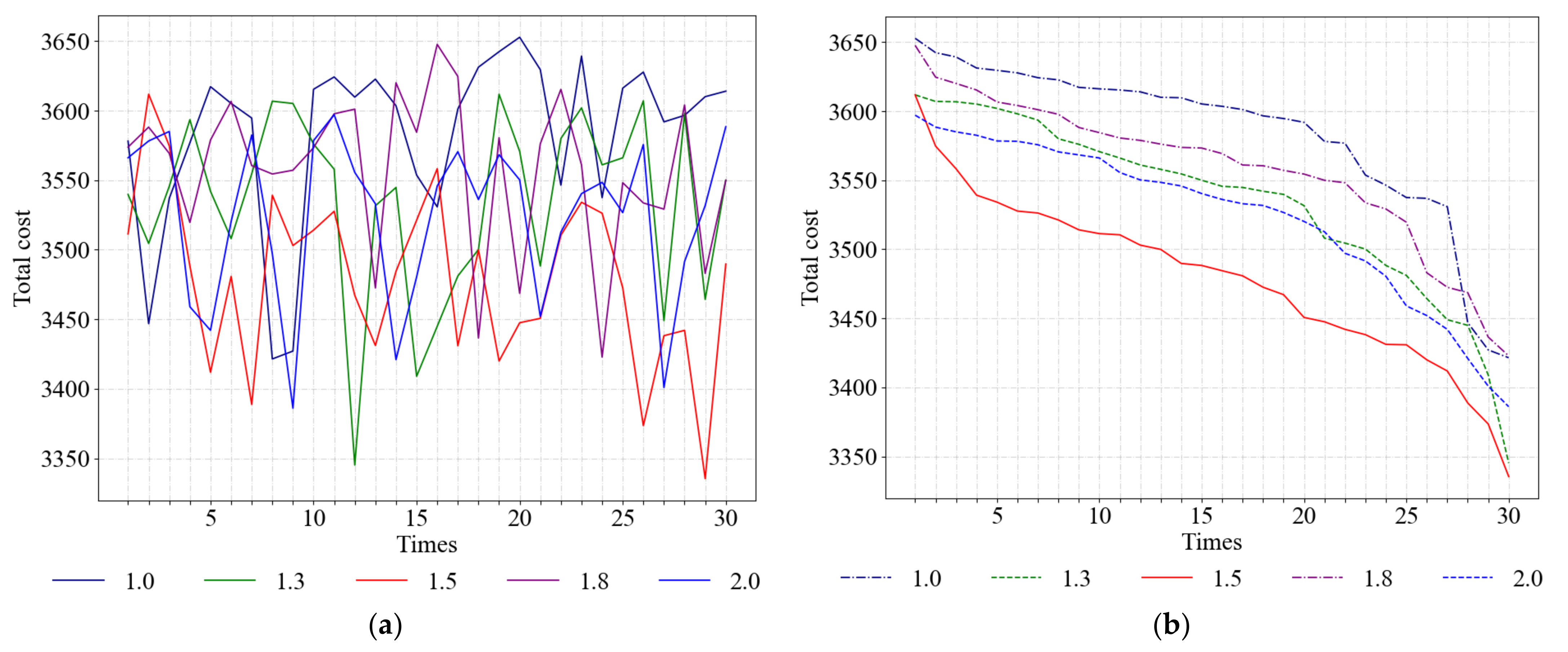
5.2.2. Value of Parameter λ
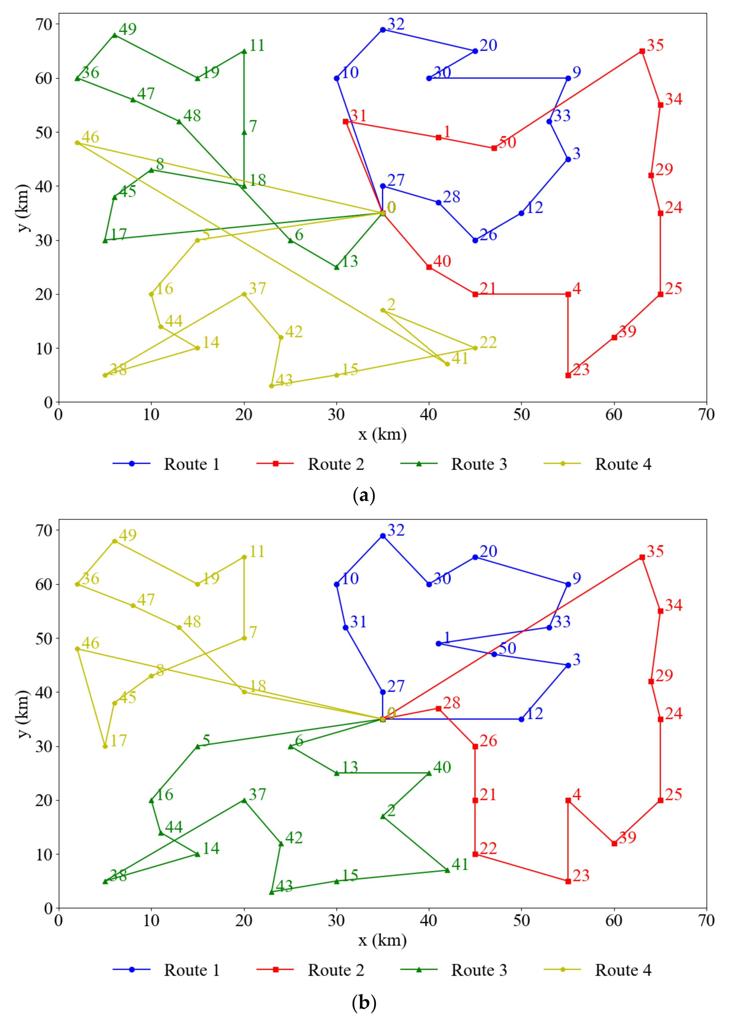
5.3. Validity Analysis of the Model
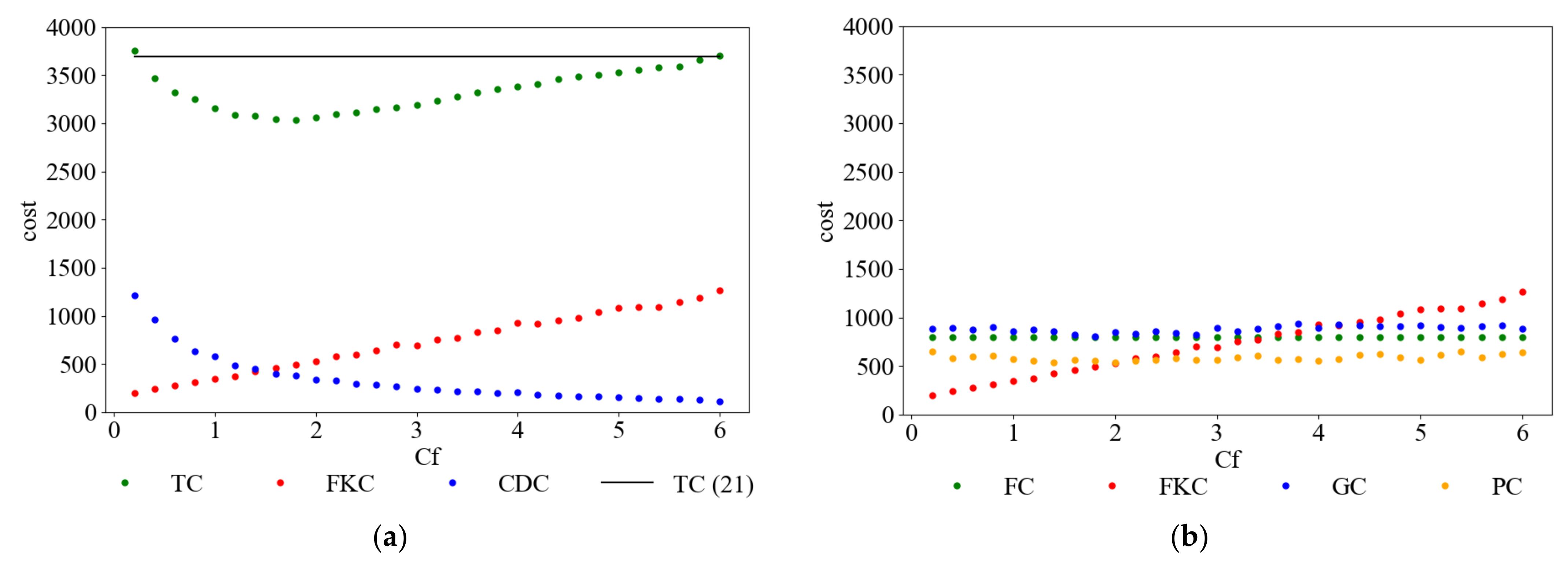
5.4. Analysis of Parameters
5.4.1. βf Is Certain
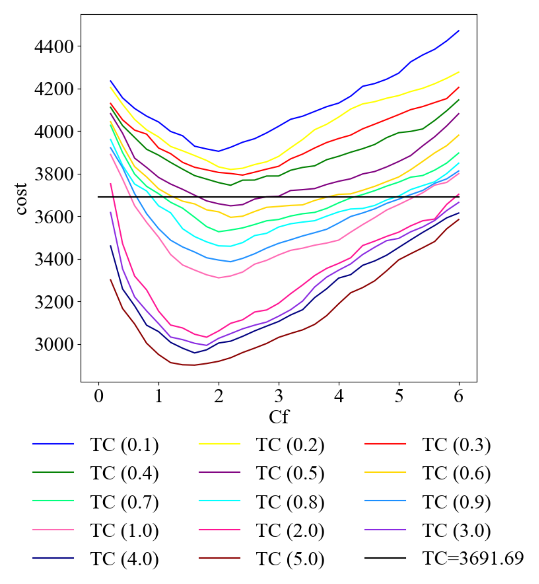
5.4.2. βf Is Not Certain
6. Conclusions
Author Contributions
Funding
Institutional Review Board Statement
Informed Consent Statement
Data Availability Statement
Conflicts of Interest
References
- Nunes, M.C.D. Correlations between subjective quality and physicochemical attributes of fresh fruits and vegetables. Postharvest Biol. Technol. 2015, 107, 43–54. [Google Scholar] [CrossRef]
- Nelson, S.O. Quality Sensing in Fruits and Vegetables. Dielectr. Prop. Agric. Mater. Their Appl. 2015, 5, 123. [Google Scholar]
- Qiu, F.; Zhang, G.; Chen, P.K.; Wang, C.; Pan, Y.; Sheng, X.; Kong, D. A Novel Multi-Objective Model for the Cold Chain Logistics Considering Multiple Effects. Sustainability 2020, 12, 8068. [Google Scholar] [CrossRef]
- Zhang, Y.; Hua, G.W.; Cheng, T.C.E.; Zhang, J.L. Cold chain distribution: How to deal with node and arc time windows? Ann. Op. Res. 2020, 291, 1127–1151. [Google Scholar] [CrossRef]
- Ma, X.; Liu, T.; Yang, P.; Jiang, R. Vehicle routing optimization model of cold chain logistics based on stochastic demand. J. Syst. Simul. 2016, 28, 1824–1832. [Google Scholar]
- Hsu, C.-I.; Hung, S.-F.; Li, H.-C. Vehicle routing problem with time-windows for perishable food delivery. J. Food Eng. 2007, 80, 465–475. [Google Scholar] [CrossRef]
- Song, M.X.; Li, J.Q.; Han, Y.Q.; Han, Y.Y.; Liu, L.L.; Sun, Q. Metaheuristics for solving the vehicle routing problem with the time windows and energy consumption in cold chain logistics. Appl. Soft Comput. 2020, 95, 15. [Google Scholar] [CrossRef]
- Meneghetti, A.; Ceschia, S. Energy-efficient frozen food transports: The Refrigerated Routing Problem. Int. J. Prod. Res. 2019, 58, 4164–4181. [Google Scholar] [CrossRef]
- Zhang, L.Y.; Tseng, M.L.; Wang, C.H.; Xiao, C.; Fei, T. Low-carbon cold chain logistics using ribonucleic acid-ant colony optimization algorithm. J. Clean. Prod. 2019, 233, 169–180. [Google Scholar] [CrossRef]
- Chen, J.; Dan, B.; Shi, J. A variable neighborhood search approach for the multi-compartment vehicle routing problem with time windows considering carbon emission. J. Clean. Prod. 2020, 277, 14. [Google Scholar] [CrossRef]
- Li, Y.; Lim, M.K.; Tseng, M.L. A green vehicle routing model based on modified particle swarm optimization for cold chain logistics. Ind. Manag. Data Syst. 2019, 119, 473–494. [Google Scholar] [CrossRef]
- Ren, X.Y. Path Optimization of Cold Chain Distribution with Multiple Distribution Centers Considering Carbon Emissions. Appl. Ecol. Environ. Res. 2019, 17, 9437–9453. [Google Scholar] [CrossRef]
- Wang, S.; Tao, F.; Shi, Y.; Wen, H. Optimization of Vehicle Routing Problem with Time Windows for Cold Chain Logistics Based on Carbon Tax. Sustainability 2017, 9, 694. [Google Scholar] [CrossRef] [Green Version]
- Qin, G.; Tao, F.; Li, L. A Vehicle Routing Optimization Problem for Cold Chain Logistics Considering Customer Satisfaction and Carbon Emissions. Int. J. Environ. Res. Public Health 2019, 16, 576–592. [Google Scholar] [CrossRef] [Green Version]
- Leng, L.; Zhang, C.; Zhao, Y.; Wang, W.; Zhang, J.; Li, G. Biobjective low-carbon location-routing problem for cold chain logistics: Formulation and heuristic approaches. J. Clean. Prod. 2020, 273, 122801. [Google Scholar] [CrossRef]
- Liu, G.; Hu, J.; Yang, Y.; Xia, S.; Lim, M.K. Vehicle routing problem in cold Chain logistics: A joint distribution model with carbon trading mechanisms. Resour. Conserv. Recycl. 2020, 156, 104715. [Google Scholar] [CrossRef]
- Babagolzadeh, M.; Shrestha, A.; Abbasi, B.; Zhang, Y.; Woodhead, A.; Zhang, A. Sustainable cold supply chain management under demand uncertainty and carbon tax regulation. Transp. Res. Part. D Transp. Environ. 2020, 80, 102245. [Google Scholar] [CrossRef]
- Galarcio-Noguera, J.D.; Riaño, H.E.H.; Pereira, J.M.L. Hybrid PSO-TS-CHR algorithm applied to the vehicle routing problem for multiple perishable products delivery. Appl. Comput. Sci. Eng. 2018, 916, 61–72. [Google Scholar]
- Hsiao, Y.H.; Chen, M.C.; Chin, C.L. Distribution planning for perishable foods in cold chains with quality concerns: Formulation and solution procedure. Trends Food Sci. Technol. 2017, 61, 80–93. [Google Scholar] [CrossRef]
- Tsang, Y.P.; Choy, K.L.; Wu, C.H.; Ho, G.T.S.; Lam, H.Y.; Tang, V. An intelligent model for assuring food quality in managing a multi-temperature food distribution centre. Food Control. 2018, 90, 81–97. [Google Scholar] [CrossRef]
- Bogataj, D.; Bogataj, M.; Hudoklin, D. Mitigating risks of perishable products in the cyber-physical systems based on the extended MRP model. Int. J. Prod. Econ. 2017, 193, 51–62. [Google Scholar] [CrossRef]
- Fikar, C. A decision support system to investigate food losses in e-grocery deliveries. Comput. Ind. Eng. 2018, 117, 282–290. [Google Scholar] [CrossRef]
- Goel, R.; Maini, R. A hybrid of ant colony and firefly algorithms (HAFA) for solving vehicle routing problems. J. Comput. Sci. 2018, 25, 28–37. [Google Scholar] [CrossRef]
- Zhang, H.; Zhang, Q.; Ma, L.; Zhang, Z.; Liu, Y. A hybrid ant colony optimization algorithm for a multi-objective vehicle routing problem with flexible time windows. Inf. Sci. 2019, 490, 166–190. [Google Scholar] [CrossRef]
- Zhang, S.; Gajpal, Y.; Appadoo, S.S.; Abdulkader, M.M.S. Electric vehicle routing problem with recharging stations for minimizing energy consumption. Int. J. Prod. Econ. 2018, 203, 404–413. [Google Scholar] [CrossRef]
- Chen, S.M.; Chien, C.Y. Solving the traveling salesman problem based on the genetic simulated annealing ant colony system with particle swarm optimization techniques. Expert Syst. Appl. 2011, 38, 14439–14450. [Google Scholar] [CrossRef]
- Deng, W.; Xu, J.; Zhao, H. An Improved Ant Colony Optimization Algorithm Based on Hybrid Strategies for Scheduling Problem. IEEE Access 2019, 7, 20281–20292. [Google Scholar] [CrossRef]
- Ajeil, F.H.; Ibraheem, I.K.; Azar, A.T.; Humaidi, A.J. Grid-Based Mobile Robot Path Planning Using Aging-Based Ant Colony Optimization Algorithm in Static and Dynamic Environments. Sensors 2015, 107, 43–54. [Google Scholar] [CrossRef] [Green Version]
- Liu, X.F.; Zhan, Z.H.; Deng, J.D.; Li, Y.; Gu, T.; Zhang, J. An Energy Efficient Ant Colony System for Virtual Machine Placement in Cloud Computing. IEEE Trans. Evolut. Comput. 2018, 22, 113–128. [Google Scholar] [CrossRef] [Green Version]
- Ottmar, R.D. Wildland fire emissions, carbon, and climate: Modeling fuel consumption. For. Ecol. Manag. 2014, 317, 41–50. [Google Scholar] [CrossRef]
- Lakshmisha, I.P.; Ravishankar, C.N.; Ninan, G.; Mohan, C.O.; Gopal, T.K.S. Effect of freezing time on the quality of Indian mackerel (Rastrelliger kanagurta) during frozen storage. J. Food Sci. 2018, 73, S345–S353. [Google Scholar] [CrossRef] [PubMed]
- Chen, J.; Dong, M. Research on shipment consolidation policy for pershable products by considering shipping freshness requirement. Syst. Eng. Theory Pract. 2018, 38, 2018–2031. [Google Scholar]


| Parameters/Variables | Descriptions |
|---|---|
| N | The number of customers. |
| K | The number of delivery vehicles in the distribution center. |
| fk | The fixed cost of each delivery vehicle. |
| X | The cargo load of the delivery vehicle. |
| Q | The maximum load capacity of the delivery vehicle. |
| Qij | The cargo carrying capacity of the delivery vehicle from customer i to customer j. |
| qi | The number of fresh agricultural products required by customer i. |
| Qin | The load capacity of the vehicle when it leaves customer i. |
| P | The unit price of fresh agricultural products. |
| The time point when the delivery vehicle k arrives at customer i. | |
| The time point when vehicle k departs from the distribution center. | |
| The driving time of vehicle k from customer i to customer j. | |
| Ti | The service time of customer i. |
| Lj | The earliest arrival time customer j can accept. |
| Rj | The latest arrival time customer j can accept. |
| η1 | The freshness attenuation coefficient when not investing the freshness-keeping cost during the driving process of the distribution vehicle. |
| η2 | The freshness attenuation coefficient when not investing the freshness-keeping cost during the unloading process of the distribution vehicle. |
| ε1 | The default cost coefficient for the delivery vehicle arriving earlier than the required time window of customers. |
| ε2 | The default cost coefficient for the delivery vehicle arriving later than the required time window of customers. |
| ρ | The fuel consumption per unit distance of the vehicles. |
| dij | The distance between customer i and the customer j. |
| cfuel | The price of the fuel. |
| υ | The carbon tax. |
| ω | The CO2 emission coefficient. |
| a | The refrigerant consumption coefficient when the vehicle is driving. |
| b | The refrigerant consumption coefficient when the vehicle is unloading goods. |
| x0ik | A binary variable that is 1 if the distribution center uses vehicle k to complete the distribution tasks, and 0 otherwise. |
| xijk | A binary variable that is 1 if vehicle k drives directly from customer i to customer j, and 0 otherwise. |
| yik | A binary variable that is 1 if the distribution demand of customer i is satisfied by vehicle k, and 0 otherwise. |
| Parameters | Values |
|---|---|
| P | 12 yuan/kg |
| η1 | 0.005 |
| η2 | 0.01 |
| ε1 | 20 yuan/h |
| ε2 | 20 yuan/h |
| a | 5 yuan/h |
| b | 12 yuan/h |
| ρ0 | 0.18 L/km |
| ρ* | 0.41L/km |
| υ | 2.669 kg/L |
| ω | 0.03 yuan/kg |
| cfuel | 5.41 yuan/L |
| Algorithm | Max | Min | Mean | Standard Deviation | Coefficient of Variation |
|---|---|---|---|---|---|
| A* | 5329.01 | 5329.01 | 5329.01 | 0 | 0 |
| ACO | 3764.07 | 3487.21 | 3619.59 | 80.47 | 0.0222 |
| HACO | 3611.81 | 3335.50 | 3479.53 | 60.02 | 0.0173 |
| λ | Max | Min | Mean | Standard Deviation | Coefficient of Variation |
|---|---|---|---|---|---|
| 1.0 | 3652.76 | 3421.50 | 3583.37 | 59.65 | 0.0166 |
| 1.3 | 3611.80 | 3345.22 | 3534.64 | 63.62 | 0.018 |
| 1.5 | 3611.81 | 3335.50 | 3479.53 | 60.02 | 0.0173 |
| 1.8 | 3647.63 | 3422.83 | 3557.97 | 54.18 | 0.0152 |
| 2.0 | 3597.10 | 3386.08 | 3524.07 | 57.49 | 0.0163 |
| Equation | Minimum Cost (yuan) | Distribution Routes Corresponding to the Minimum Cost |
|---|---|---|
| (21) | 3691.69 | [0, 27, 28, 26, 12, 3, 33, 9, 30, 20, 32, 10, 0] [0, 40, 21, 4, 23, 39, 25, 24, 29, 34, 35, 50, 1, 31, 0] [0, 13, 6, 48, 47, 36, 49, 19, 11, 7, 18, 8, 45, 17, 0] [0, 5, 16, 44, 14, 38, 37, 42, 43, 15, 22, 2, 41, 46, 0] |
| (30) | 3335.5 | [0, 27, 31, 10, 32, 30, 20, 9, 33, 1, 50, 3, 12, 0] [0, 28, 26, 21, 22, 23, 4, 39, 25, 24, 29, 34, 35, 0] [0, 5, 16, 44, 14, 38, 37, 42, 43, 15, 41, 2, 40, 13, 6, 0] [0, 18, 48, 47, 36, 49, 19, 11, 7, 8, 45, 17, 46, 0] |
| Equation | TC | FC | GC | FKC/RC | CDC | PC |
|---|---|---|---|---|---|---|
| (21) | 3691.69 | 800 | 919.28 | 204.10 | 1166.18 | 602.13 |
| (30) | 3335.50 | 800 | 882.86 | 252.26 | 824.70 | 575.68 |
| Equation (21) | Equation (30) | ||||
|---|---|---|---|---|---|
| Component | Amount (yuan) | Proportion (%) | Component | Amount (yuan) | Proportion (%) |
| TC | 3691.69 | 100 | TC | 3335.50 | 100 |
| FC | 800 | 21.67 | FC | 800 | 23.98 |
| GC | 919.28 | 24.90 | GC | 882.86 | 26.49 |
| RC | 204.10 | 5.53 | FKC | 252.26 | 7.56 |
| CDC | 1166.18 | 31.59 | CDC | 824.70 | 24.72 |
| PC | 602.13 | 16.31 | PC | 575.68 | 17.25 |
| TC | FC | GC | FKC | CDC | PC | |
|---|---|---|---|---|---|---|
| 0.2 | 3752.96 | 800 | 885.12 | 201.24 | 1214.48 | 652.12 |
| 0.4 | 3471.44 | 800 | 893.57 | 239.3 | 958.95 | 579.62 |
| 0.6 | 3319.57 | 800 | 879.48 | 276.9 | 764.27 | 598.92 |
| 0.8 | 3254.61 | 800 | 905.68 | 311.58 | 631.79 | 605.56 |
| 1.0 | 3154.69 | 800 | 855.26 | 348.51 | 580.98 | 569.94 |
| 1.2 | 3089.37 | 800 | 874.17 | 375.22 | 483.82 | 556.16 |
| 1.4 | 3075.68 | 800 | 860.28 | 423.13 | 452.2 | 540.07 |
| 1.6 | 3046.23 | 800 | 820.29 | 460.61 | 399.87 | 565.46 |
| 1.8 | 3032.28 | 800 | 802.05 | 498.26 | 378.65 | 553.32 |
| 2.0 | 3061.62 | 800 | 852.48 | 529.94 | 340.98 | 538.22 |
| 2.2 | 3097.39 | 800 | 834.6 | 581.73 | 329.08 | 551.98 |
| 2.4 | 3114.02 | 800 | 854.6 | 599.58 | 294.8 | 565.04 |
| 2.6 | 3150.49 | 800 | 843.12 | 639.74 | 286.29 | 581.34 |
| 2.8 | 3160.21 | 800 | 823.78 | 704.13 | 271.02 | 561.28 |
| 3.0 | 3191.57 | 800 | 893.17 | 697.23 | 239.25 | 561.92 |
| 3.2 | 3236.56 | 800 | 859.62 | 753.32 | 232.46 | 591.16 |
| 3.4 | 3277.69 | 800 | 880.97 | 770.51 | 218.29 | 607.92 |
| 3.6 | 3321.75 | 800 | 907.69 | 834.19 | 213.53 | 566.34 |
| 3.8 | 3355.48 | 800 | 934.43 | 846.52 | 199.21 | 575.32 |
| 4.0 | 3378.92 | 800 | 889.26 | 928.59 | 205.27 | 555.8 |
| 4.2 | 3405.15 | 800 | 931.34 | 915.96 | 182.07 | 575.78 |
| 4.4 | 3462.71 | 800 | 919.82 | 957.46 | 173.61 | 611.82 |
| 4.6 | 3483.32 | 800 | 913.83 | 977.08 | 164.86 | 627.55 |
| 4.8 | 3505.86 | 800 | 913.26 | 1040.39 | 163.67 | 588.54 |
| 5.0 | 3525.46 | 800 | 921.85 | 1080.45 | 158.93 | 564.23 |
| 5.2 | 3555.31 | 800 | 904.15 | 1088.01 | 148.34 | 614.81 |
| 5.4 | 3579.08 | 800 | 897.17 | 1091.59 | 139.76 | 650.56 |
| 5.6 | 3587.24 | 800 | 909.94 | 1143.57 | 142.96 | 590.77 |
| 5.8 | 3656.02 | 800 | 914.77 | 1184.22 | 129.65 | 627.38 |
| 6.0 | 3703.37 | 800 | 887.85 | 1264.32 | 113.3 | 637.9 |
Publisher’s Note: MDPI stays neutral with regard to jurisdictional claims in published maps and institutional affiliations. |
© 2021 by the authors. Licensee MDPI, Basel, Switzerland. This article is an open access article distributed under the terms and conditions of the Creative Commons Attribution (CC BY) license (https://creativecommons.org/licenses/by/4.0/).
Share and Cite
Zhu, S.; Fu, H.; Li, Y. Optimization Research on Vehicle Routing for Fresh Agricultural Products Based on the Investment of Freshness-Keeping Cost in the Distribution Process. Sustainability 2021, 13, 8110. https://doi.org/10.3390/su13148110
Zhu S, Fu H, Li Y. Optimization Research on Vehicle Routing for Fresh Agricultural Products Based on the Investment of Freshness-Keeping Cost in the Distribution Process. Sustainability. 2021; 13(14):8110. https://doi.org/10.3390/su13148110
Chicago/Turabian StyleZhu, Shenjun, Hongming Fu, and Yanhui Li. 2021. "Optimization Research on Vehicle Routing for Fresh Agricultural Products Based on the Investment of Freshness-Keeping Cost in the Distribution Process" Sustainability 13, no. 14: 8110. https://doi.org/10.3390/su13148110
APA StyleZhu, S., Fu, H., & Li, Y. (2021). Optimization Research on Vehicle Routing for Fresh Agricultural Products Based on the Investment of Freshness-Keeping Cost in the Distribution Process. Sustainability, 13(14), 8110. https://doi.org/10.3390/su13148110