Article

El Niño, La Niña, and the Forecastability of the Realized Variance of Heating Oil Price Movements

1
Department of Economics, Eastern Mediterranean University, Famagusta 99268, Turkey
2
Adnan Kassar School of Business, Lebanese American University, Beirut P.O. Box 13-5053, Lebanon
3
Department of Economics, University of Pretoria, Pretoria 0002, South Africa
4
Department of Economics, Helmut Schmidt University, 22008 Hamburg, Germany
*
Author to whom correspondence should be addressed.
Sustainability 2021, 13(14), 7987; https://doi.org/10.3390/su13147987
Submission received: 4 June 2021 / Revised: 7 July 2021 / Accepted: 9 July 2021 / Published: 16 July 2021
(This article belongs to the Special Issue Energy Transition amidst Global Energy Demand and Trade Studies)

Abstract

:
We use the heterogenous autoregressive (HAR) model to compute out-of-sample forecasts of the monthly realized variance (RV) of movements of the spot and futures price of heating oil. We extend the HAR–RV model to include the role of El Niño and La Niña episodes, as captured by the Equatorial Southern Oscillation Index (EQSOI). Using data from June 1986 to April 2021, we show evidence for several model configurations that both El Niño and La Niña phases contain information useful for forecasting subsequent to the realized variance of price movements beyond the predictive value already captured by the HAR–RV model. The predictive value of La Niña phases, however, seems to be somewhat stronger than the predictive value of El Niño phases. Our results have important implications for investors, as well as from the perspective of sustainable decisions involving the environment.

1. Introduction

As pointed out by Trenberth et al. [1], the El Niño Southern Oscillation (ENSO) is an irregularly periodic variation in winds and sea surface temperatures over the tropical eastern Pacific Ocean, which, in turn, impacts the climate of much of the tropical and subtropical zones. In this regard, the warming phase of the sea temperature is known as El Niño, while the cooling phase is called La Niña, with the two phases lasting several months each and typically occurring every few years with varying intensities. Because El Niño phases tend to be warmer and drier overall, people will require less heating and more cooling, while the opposite is true for La Niña phases. As a result, El Niño and La Niña phases are likely to cause fluctuations in the price of heating oil, given its crucial role as a source of heat in the winter months. Not surprisingly, while analyzing the role of the ENSO on the prices of oil, gasoline, heating oil, diesel fuel, jet fuel and propane, [2] detect the strongest impact for heating oil.
Against the backdrop, we build on this line of research by verifying whether this evidence of the impact of ENSO on the first moment of the price of heating oil can be extended to out-of-sample forecasting of its second moment (that is, the variance of price movements), which is likely to be affected via variable demand for heating oil during El Niño and La Niña phases, associated with extreme warm and cold temperatures during a year. In this regard, we can further hypothesize that with the La Niña events associated with extreme cold weather, they are likely to have a relatively stronger influence on the volatility of heating oil than the corresponding El Niño phases. Moreover, the ENSO has been held (partially) responsible for some of the world’s greatest humanitarian disasters, with [3,4] documenting the global El Niño droughts of 1876–1878, 1888–1891, and 1896–1902, which contributed to the deaths of between 30 and 60 million people in India, China and Brazil over the 26 year period. Moreover, these extreme weather conditions can constrain the supply of rain-driven agricultural commodities and induce food price and generalized inflation [5,6,7,8], which may trigger social unrest as shown empirically by [9] and both theoretically and empirically in [10]. In this regard, [11,12,13,14] show that El Niño and La Niña shocks may even have played a role in a substantial number of civil conflicts. In this sense, the ENSO cycle can serve as a proxy for rare disaster risks [15], which in turn contribute to jump risks [16,17] that account for a large part of the volatility process of asset and commodity prices [18,19,20]. Naturally, one can expect an impact on the variance of price movements of heating oil via the volatility jumps channel as well, over and above the heating oil demand fluctuations route due to El Niño and La Niña events.
Yet, from a statistical perspective, it is well-established that in-sample predictability does not necessarily guarantee out-of-sample predictability gains emerging from a specific predictor, and it is in fact the latter approach that often provides a more robust test of the appropriateness of an econometric model [21]. Hence, rather than focusing on in-sample predictions, we use an out-of-sample forecasting experiment to test the predictive value of El Niño and La Niña for the variance of movements of the price of heating oil. At the same time, heating oil is second only to gasoline in terms of products derived from crude oil, and given that commodity market participants need real-time volatility forecasts for effective investment, hedging risk and arbitrage strategies, the economic importance of the question we ask in this paper cannot be overemphasized. This is more so given the close linkage between energy-based commodities and the financial markets in the wake of the process of financialization of the former, and with investors looking for alternative safe investment assets following the Global Financial Crisis (see, for example, [22,23] for detailed discussions in this regard).
Given this, we forecast the monthly realized variance (RV) of movements of the spot and future heating oil price using an extended version of the widely-studied heterogeneous autoregressive (HAR)–RV model [24]. We extend the model to incorporate the role of El Niño and La Niña phases that occurred during the period from June 1986 to April 2021. In this regard, it is important to note that measuring variance in terms of RV, defined as the sum of squared daily returns of prices observed over a given month (see [25]), provides an observable and unconditional metric of variance, which is otherwise a latent process. Accordingly, we differ from the existing literature (see for example, [26,27,28,29,30,31,32]) on modeling and forecasting heating oil volatility based on various types of univariate GARCH models, under which the conditional variance is a deterministic function of model parameters and historical data, and, hence, is not model-free as in the case of RV. Moreover, as discussed in [33,34], the benchmark HAR–RV model captures the generally observed long-memory and multi-scaling properties of volatility, despite having a simplistic structure. Notably, one important feature of the HAR–RV model is that it employs volatilities from different time resolutions to forecast the realized heating oil price volatility. Accordingly, the model captures the main idea motivating the heterogeneous market hypothesis (EMH, [35]) in a simple and straightforward way. The EMH indicates that different groups of market participants populate financial markets (that is, in our case, the market for heating oil), and that these groups differ in their sensitivity to information flows at various time horizons. For example, in the energy market, speculators and traders are concerned with short-term investment horizons, whereas institutional investors are concerned with long-term investment horizons.
At this stage, to emphasize our contribution, it is important that we provide some further details on the literature cited above dealing with heating oil volatility forecasting, with these studies also simultaneously often dealing with crude oil, natural gas and gasoline. While in what follows we present a brief outline of the existing literature on forecasting heating oil price volatility, the reader is referred to [36] for a more detailed discussion of the literature on volatility forecasting of multiple energy commodities.
In this regard, Sadorsky cite26 showed that within the GARCH family models, the threshold GARCH (TGARCH) framework proved to be the most appropriate for the volatility of heating oil futures returns over the daily periods from 1988 to 2003. Nomikos and Pouliasis [27] compared the forecasting ability of a Markov-Switching (MS)–GARCH model to the basic GARCH on a dataset containing information about daily futures prices from 1991 to 2008 for heating oil, to depict the dominance of the former due to its ability to account for the special volatility characteristics. Arouri [28], while analyzing both daily spot and futures prices from 1986 to 2011, highlighted the role of a Fractionally Integrated GARCH (FIGARCH) model in its ability to better describe the time-varying volatility process, as it can capture long-memory (which decreases after incorporating structural breaks), a phenomenon we also account for via the HAR–RV model. Given this, the FIGARCH model (suitably modified to account for structural breaks) is shown to perform better than any other related model in forecasting heating oil volatility. Along similar lines, ref. [29] showed that the Autoregressive Fractionally Integrated Moving Average (ARFIMA)-FIGARCH model dominated various other GARCH-class models in forecasting volatility for heating oil derived from daily futures data covering 1995–2012. Different to the existing studies, ref. [31] pointed out that the unbiased extreme value volatility estimator, namely the Add RS, when incorporated into an ARFIMA model of heating oil futures volatility, outperforms the alternative models from the GARCH family over the daily period from 1996 to 2013. In a similar vein, in terms of methodological innovation, ref. [32] compared support vector regression (SVR) with the GARCH models, and showed the superiority of the former approach in forecasting the volatility of heating oil futures based on daily data from 2015 to 2019. However, this study also indicated that, within the GARCH models, asymmetric versions tend to perform better—an observation drawn earlier by [26]. Interestingly, while all the above studies relied on univariate models, ref. [30] stressed the need to look at multivariate (the Full BEKK [37], the Diagonal BEKK and Scalar BEKK) models while forecasting weekly spot prices of heating oil, as these frameworks capture the time-varying correlation between the returns processes of the energy-based commodities.
Given the brief description of the academic literature, it appears that our current paper is the first paper that evaluates the out-of-sample forecasting power of the El Niño and La Niña phases for the realized variance of heating oil price movements, which are likely to be affected via demand and volatility jumps channels, based on an extended HAR–RV model. Our focus is not necessarily to contribute to the technicality of volatility forecasting models, but rather to consider the usage of innovative predictors, namely the El Niño and La Niña phases.
Section 2 provides the dataset. Section 3 describes the HAR–RV model. Section 4 presents the results from our forecasting experiment. Section 5 concludes the paper.

2. Data

We use daily spot and futures prices of heating oil (U.S. dollars and cents per gallon) as represented by the New York Harbor No. 2 Heating Oil Spot Price FOB and the continuous NYMEX New York HARBOR ULSD futures contract, respectively, with the price data extracted from DataStream. After having computed the continuously compounded (i.e., log) daily returns of the spot and futures prices, we compute the monthly realized variance by taking the sum of daily squared returns over a month, where the overall sample period runs from June 1986 to April 2021. Figure 1 shows the daily price data that we used to construct the monthly realized variances. Table 1 depicts the key summary statistics of daily returns. Both returns series are slightly negatively skewed, are leptokurtic and they are slightly positively (negatively) skewed in the case of spot (futures) returns. The two top panels of Figure 2 show the monthly realized variances of the spot and futures returns of the heating oil price. While the overall pattern of RV is similar across the spot and futures data, there are also noticeable differences visible in the figure, for example, in the early 1990s, in 2000 and in 2020 at the end of the sample period.
In order to measure the ENSO cycle, we rely on the Southern Oscillation Index (SOI) as compiled and published by the Bureau of Meteorology, Government of Australia (http://www.bom.gov.au/climate/current/soihtm1.shtml, accessed on 21 May 2021). The SOI summarizes the development and intensity of El Niño or La Niña events in the Pacific Ocean. From a methodological point of view, the SOI is computed by taking the pressure differences between Tahiti and Darwin. Such pressure differences are important because low atmospheric pressure tends to occur over warm water, while high pressure tends to occur over cold water, in part because of deep convection over the warm water. El Niño phases are, by definition, periods of sustained warming of the central and eastern tropical Pacific Ocean. La Niña phases are periods of sustained cooling of the central and eastern tropical Pacific Ocean. As such, the result is a decrease and an increase in the strength of the Pacific trade winds, respectively. Sustained negative (positive) realizations of the SOI below (above) −7 (+7) usually indicate El Niño (La Niña) phases.
It should be mentioned, however, that a drawback of the SOI data is because both Darwin and Tahiti are located well south of the Equator, implying that the surface air pressure at both locations is less directly linked to ENSO. In order to address this drawback, a new index called the Equatorial Southern Oscillation Index (EQSOI) was constructed. For further details, see https://www.climate.gov/news-features/blogs/enso/why-are-there-so-many-enso-indexes-instead-just-one (accessed on 21 May 2021). The data for this index are collected at two new regions, both centered on the Equator, where the western one is located over Indonesia while the eastern one is located over the equatorial Pacific, close to the South American coast. We collect data on the EQSOI from the Climate Prediction Center of the National Oceanic and Atmospheric Administration (US Department of Commerce). See https://www.cpc.ncep.noaa.gov/data/indices/ (accessed on 21 May 2021).
Like [38], we first compute the SOI and EQSOI “anomalies”, defined as the deviation of the SOI and EQSOI in any given month from its historical average, normalized (divided) by its historical standard deviation. The two middle panels of Figure 2 show the EQSOI data and the EQSOI anomaly. Equipped with the anomalies, we identify sustained negative SOI and EQSOI anomaly values below −1 (above +1) as indicators of El Niño (La Niña) phases. In order to capture the two phases of the ENSO cycle, we create a dummy variable which assumes the value of one whenever the SOI and EQSOI anomalies are negative (positive), and zero otherwise. Finally, we multiply the dummy variable with the SOI and EQSOI anomalies to obtain a metric for the intensity of the El Niño (La Niña) phases. In our empirical analysis, we use the El Niño and La Niña phases, depicted in the two lower panels of Figure 2, associated with EQSOI as a measure of the ENSO, given its stronger reliability. We use the El Niño and La Niña phases based on the SOI data for a robustness check.

3. The HAR–RV Model

The HAR–RV model proposed by [24] has become the workhorse model in empirical finance for the analysis of the dynamics of the realized variance ( R V ) of asset-price returns. While the HAR–RV model is typically applied to studying high-frequency data, we use a variant of the HAR–RV model to study the monthly realized variance ( R V ) of spot and futures movements of the price of heating oil. Our benchmark HAR–RV model is given by:
R V t + h = β 0 + β 1 R V t + β 2 R V q , t + β 3 R V y , t + ϵ t + h ,
where h = the forecast horizon, R V t + h = the average (spot or futures) realized variance observed during the forecast horizon, R V q , t = the average quarterly realized variance from month t 3 to t 1 , and R V y , t = the average yearly realized variance from month t 12 to t 1 ). We estimate the following coefficients β j , j = 0 , 1 , 2 , 3 , and ϵ t = a disturbance term.
The predictive value of the benchmark HAR–RV model is compared to that of each of the following extended HAR–RV models:
R V t + h = β 0 + β 1 R V t + β 2 R V q , t + β 3 R V y , t + β 4 El   Niño t + ϵ t + h ,
R V t + h = β 0 + β 1 R V t + β 2 R V q , t + β 3 R V y , t + β 5 La   Niña t + ϵ t + h ,
R V t + h = β 0 + β 1 R V t + β 2 R V q , t + β 3 R V y , t + β 4 El   Niño t + β 5 La   Niña t + ϵ t + h .
In our empirical analysis, we focus on the out-of-sample predictive performance of our various HAR–RV models. We compute out-of-sample forecasts by estimating the models on rolling-estimation windows of different lengths. Equipped with the out-of-sample forecasts, we then evaluate the forecasts by means of the Clark and West [39] test. The null hypothesis of this test is that the two models that a researcher compares have an equal out-of-sample mean-squared prediction error (MSPE). The Clark–West test is easy to implement because it requires regressing the quantity f ^ t + h = ( R V t + h R V ^ A , t + h ) 2 [ ( R V t + h R V ^ B , t + h ) 2 ( R V ^ A , t + h R V ^ B , t + h ) 2 ] on a constant. A hat over a variable marks a forecast of R V and the subindices A and B denote the two models being compared (B denotes the larger model). We reject the null hypothesis if the t-statistic of the constant in this regression model is significantly positive (one-sided test; we use Newey–West robust standard errors to compute the t-statistic). In addition, we use the root mean squared forecasting error (RMSFE) and the mean absolute forecasting error (MAFE) statistics to compare the forecasting performance of the various HAR–RV models. We carry out our forecasting experiments using the R language for statistical computing [40].
As an extension and a robustness check (and given the results of the causality-in-quantiles test reported in Table A1 at the end of the paper), we consider a quantile-regression version of the HAR–RV model (see [41,42], among others). The quantile-regression variant of the HAR–RV model is tailored to study whether the predictive value of the El Niño and La Niña phases differs across the quantiles of the conditional distribution of the realized variance. The quantile-regression HAQR–RV model is estimated by minimizing
b ^ α = arg min t ρ α ( R V t + h X t b α ) ,
where ρ α = ϵ t + h ( α 1 ( ϵ t + h < 0 ) denotes the standard check function, α denotes a quantile, 1 denotes the indicator function, and b α denotes a vector of quantile-specific parameters to be estimated (a hat denotes an estimated parameter). In Equation (5), we simplify the notation by letting the matrix X t denote the predictors of the HAQR–RV model.
In order to evaluate forecasts for the various quantiles of the conditional distribution of R V , we use an out-of-sample relative loss criterion [43,44]. The out-of-sample relative-loss criterion, R o , is defined as:
R o = 1 t = τ T [ α + ( 1 2 α ) 1 ( R V t R V ^ t , α < 0 ) ] | R V t R V ^ t , α | p t = τ T [ α + ( 1 2 α ) 1 ( R V t R V ¯ t , α < 0 ) ] | R V t R V ¯ t , α | p ,
where R V ¯ t denotes the forecast derived from the benchmark model given in Equation (1), τ is the first period for which a forecast is available. It should be noted that the benchmark forecast is also indexed by the quantile parameter, α , showing that the benchmark model is also estimated as an HARQ–RV model.
The parameter, p, governs the functional form used to compute the out-of-sample relative loss criterion. Specifically, in case we set p = 1 , a forecaster evaluates forecast errors under a lin–lin loss function (L1; this case corresponds to the check function of the quantile regression framework), while in the case of p = 2 , a forecaster uses a quad–quad loss function (L2) to evaluate forecast errors [45].
It should be noted that the quantile parameter, α ( 0 , 1 ) , governs the asymmetry of the loss function. The loss function is symmetric for α = 0.5 and is symmetric and quadratic if, in addition, p = 2 . Setting α = 0.5 and p = 1 , in turn, implies that the the loss from a forecast error increases in the absolute magnitude of the forecast error. If α > 0.5 ( α < 0.5 ), then the loss from underpredicting (overpredicting) R V exceeds the loss from an overprediction (underprediction) of the same size, that is, for α 0.5 the loss function is asymmetric.
For a given quantile parameter and a given functional form of the loss function, the HARQ–RV model, extended to include the El Niño and/or La Niña phases, outperforms the benchmark HARQ–RV model when the out-of-sample relative loss criterion is positive, R o > 0 . When the out-of-sample relative loss criterion assumes a negative value, R o < 0 , the benchmark model performs better than the extended model.

4. Empirical Results

Table 2 summarizes our main forecasting results. We report, for the EQSOI data, results for the CW test (p-values) for different forecast horizons ( h = 1 , 3 , 6 , 12 , 24 , 36 , 48 ) and various lengths of the rolling estimation window (48, 60, 72, 96 and 120 months). In Panels A to C, we document the results for spot R V , while Panels D to F contain the results for futures R V . In the case of spot R V (Panel A), we observe that El Niño phases add to the predictive performance of the HAR–RV model when we use an intermediate window length and forecast horizons of up to two years. The test results become largely insignificant for the short and the long window length and for the longer forecast horizons. When we consider La Niña phases in Panel B, in contrast, most test results are significant. Only for a combination of a long estimation window and a short to intermediate forecast horizon are the test results not statistically significant. A similar result emerges when we combine El Niño and La Niña phases in a unified forecasting model (Panel C).
For the futures R V , the results are slightly different. The forecasting model that features El Niño phases as an additional predictor (Panel D) only adds predictive value to the HAR–RV model for the two short rolling estimation windows. The test results for the other model configurations are statistically insignificant. For La Niña phases, in contrast, the test results are stronger (Panel E). The CW test yields significant results for all combinations of window length and forecast horizon with only a few exceptions, which are not systematically linked either to the window length or the forecast horizon. It is clear, thus, that La Niña phases are an important source of the superior forecasting performance that we find in Panel F, where we consider the forecasting model that features both El Niño and La Niña phases as additional predictors.
It is interesting to examine whether the test results are robust to a change in the definition of realized variance. To this end, we report in Table 3 the test results for the square root of realized variance, R V , which researchers in empirical finance also often consider as a metric of realized “volatility”. The results that we document in Panel A witness that the contribution of El Niño phases to the predictive performance of the HAR–RV model, in the case of spot R V , is concentrated at the shorter forecast horizons. The overall picture that emerges, however, is that La Niña phases (Panel B) have a more systematic statistically significant effect on the forecasting performance of the HAR–RV model than on El Niño phases. Only the test results for the long rolling estimation window are not significant. We conclude that La Niña phases are a major driver of the results, especially as far as the longer forecast horizons are concerned, for the combined model in Panel C. For the futures-based R V (Panels D to F), the results are not too different. We observe that the contribution of El Niño phases to the forecasting performance of the HAR–RV model, in terms of statistical significance, is concentrated at the two short rolling estimation windows and at the intermediate forecast horizons. The overall picture that emerges from a comparison with the results for La Niña phases in Panel D, however, is that, with the exception of the long rolling estimation window, the test results for La Niña phases are statistically significant for a broader array of combinations of window length and forecast horizons. As a result, it is not surprising that the test results in Panel F, for a model that features both El Niño and La Niña phases as predictors, are largely significant.
Table 4 summarizes the results of an additional robustness check, where we replace our EQSOI-based predictors with corresponding predictors based on the SOI data. The results corroborate our EQSOI-based results. Most test results are statistically significant and show that accounting for El Niño and La Niña phases helps to improve forecasts of R V of heating oil price movements at various forecast horizons.
Our empirical findings show that both El Niño and La Niña have predictive value in an out-of-sample forecasting experiment for the realized variance (and volatility) of heating oil price movements, as measured by means of spot and futures price data. On balance, however, the predictive value of La Niña appears to be somewhat more robust in our out-of-sample forecasting experiment across the various model configurations that we have studied than the predictive value of El Niño. The results that we report in Table 5 illustrate this finding. Specifically, we report in Table 5 (for the EQSOI data in Panel A and the SOI data in Panel B) the average RMSFE statistics and the average ratios of the MAFE statistics as computed, for every model, across the five different lengths of the rolling-estimation window and the six different forecast horizons. The ratios are defined by dividing the RMSFE (MAFE) obtained for the baseline HAR–RV model by the corresponding RMSFE (MAFE) obtained for the HAR–RV model extended to include the El Niño and/or La Niña phases. Hence, a ratio larger than one indicates that the extended model produces, on average, more accurate forecasts than the baseline HAR–RV model. The punchline of the results summarized in Table 5 is that extending the the HAR–RV model to include El Niño phases tends to improve forecast accuracy, but extending the HAR–RV model to incorporate La Niña phases leads to a larger improvement of forecast accuracy. In fact, including both El Niño and La Niña phases in the forecasting model yields RMSFE and MAFE ratios that are close to the ratios reported for the forecasting model that features the La Niña phases as the only additional predictor.
We next turn to a quantiles-based analysis. As for in-sample predictability, we find, based on the multivariate version of the the nonparametric k-th order causality-in-quantiles test of [46], which allows us to test for causality in (spot and futures) returns and squared returns (i.e., variance) simultaneously over their respective conditional distributions (thus defining the states of the heating oil market) strong evidence of in-sample predictability from both El Niño and La Niña phases, when controlling for La Niña or El Niño in the model, respectively—see the results reported in Table A1 at the end of the paper. The results further show that the evidence of in-sample predictability is not concentrated at one or a few quantiles, justifying our decision to use the HARQ–RV model to compute quantile-specific forecasts of R V , and to use the out-of-sample relative-loss criterion to evaluate the forecasts relative to the forecasts we obtain from the benchmark HARQ–RV model. In order to save journal space, we compare the models that feature either El Niño or La Niña phases as an additional predictor.
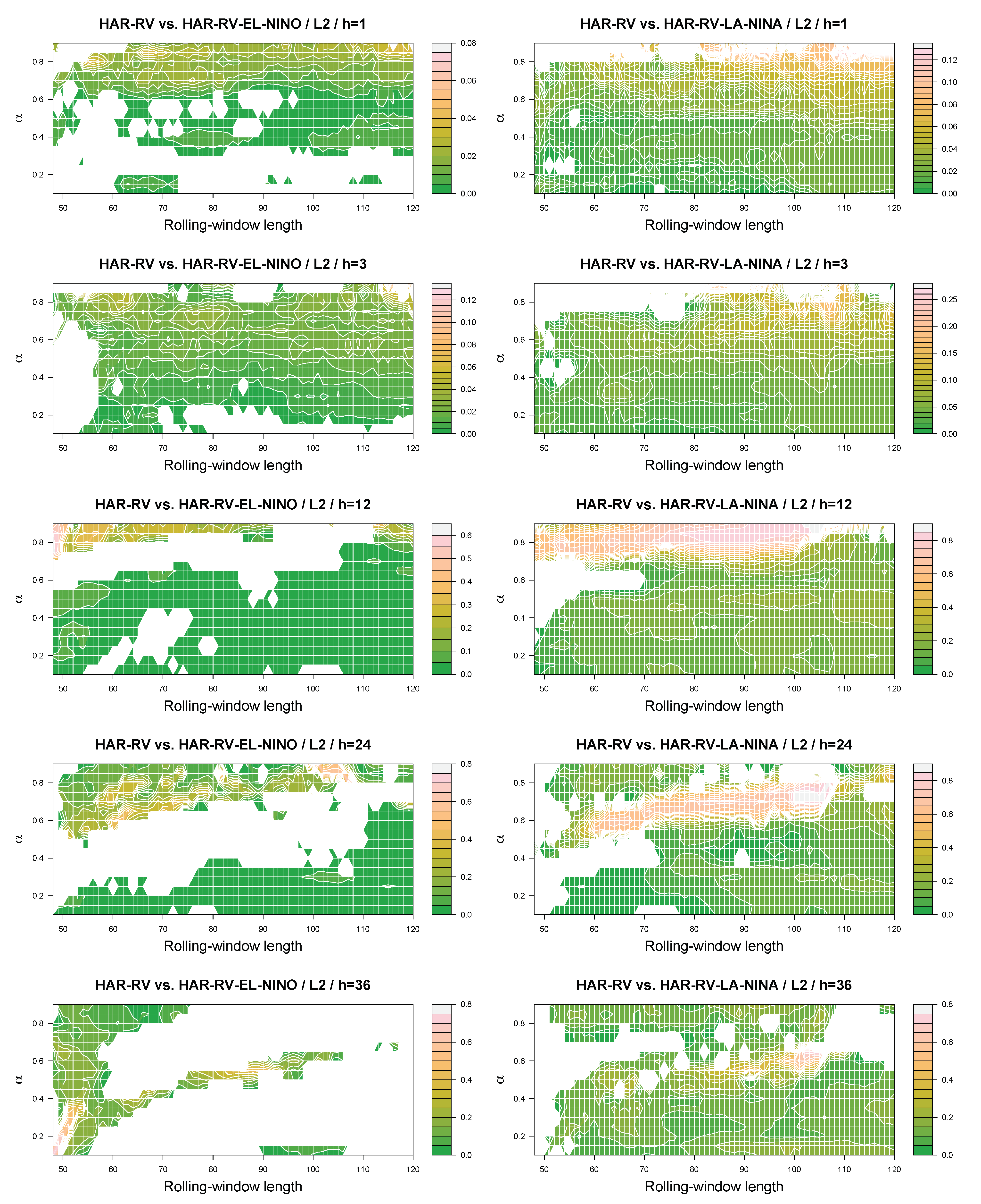
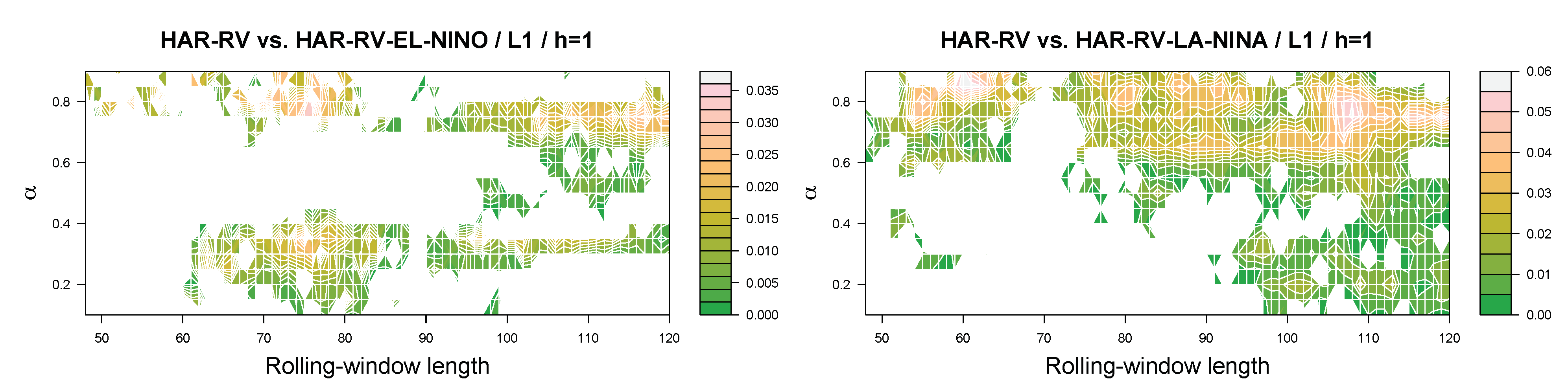
 Figure 3 and Figure 4 summarize the results for the spot R V under the lin–lin and quad–quad loss function. For the lin–lin loss function, the colored areas depicted in the figure show that, according to the out-of-sample relative-loss criterion, using El Niño phases contributes to the overall forecasting performance of the HARQ–RV model mainly at the short to intermediate forecast horizons, while the areas where the benchmark HARQ–RV model performs better than the extended model become larger as the forecast horizon increases. The results for the La Niña phases, in contrast, show that the contribution of this predictor to the forecasting performance of the model increases in terms of the out-of-sample relative-loss criterion when we study the intermediate to long forecast horizons. For the quad–quad loss function, in turn, the HARQ–RV model extended to include La Niña phases as an additional predictor outperforms the benchmark HARQ–RV model in terms of the out-of-sample relative-loss criterion for most combinations of the quantile parameter and the length of the rolling estimation window for all forecast horizons being studied. A key message conveyed by the results is that the overall contribution of La Niña phases to the forecasting performance of the model is stronger than that of El Niño phases. In this regard, it should also be noted that, as indicated by the legends of the figures, the maximum gains a forecaster can realize in terms of the out-of-sample relative-loss criterion are often larger for La Niña phases than for El Niño phases.
In this regard, we note that the higher values of the statistic for the k-th order nonparametric causality-in-quantiles test, as reported in Table A1, confirm the finding of a stronger impact of La Niña phases relative to El Niño ones, especially at higher conditional quantiles, which corresponds to higher returns and volatility. In fact, based on the average derivative (AD) using the conditional pivotal quantile, based on the approximation or the coupling approach of [47], both El Niño and La Niña phases are found to have a positive relationship with the entire conditional distributions of returns and the volatility of heating oil price. These results are available from the authors upon request.
Figure A1 and Figure A2 at the end of the paper (Appendix A) summarize the results for the futures R V . Again, we observe that the range of combinations of the quantile parameter and the length of the rolling estimation window that result in positive realizations of the out-of-sample relative-loss criterion tends to be wider for La Niña phases than for El Niño phases. Hence, to summarize, the message to take home from the results is that the out-of-sample relative loss criterion takes on positive values for many combinations of the quantile parameter, window length, and the the forecast horizon being studied, especially as far as the La Niña phases are concerned.
Finally, we present in Table 6 the results for upside (“good”) and downside (“bad”) R V , where the former is computed from positive daily returns, while the latter is computed from negative daily returns. This is an important issue, as [48] stresses that financial market participants care not only about the nature of volatility, but also about its level, with traders typically differentiating between good and bad volatilities, which, in turn, provides us the motivation to look at such disaggregation of R V . We present in Table 6 the results for the futures R V , but results for spot R V are qualitatively similar (and available from the authors upon request). The results show that El Niño phases add to the forecasting performance of the HAR–RV model estimated for upside and downside R V only for the two shortest rolling estimation windows. La Niña phases, in contrast, also carry information for several forecast horizons, which is useful for forecasting upside and downside R V when we study the longer rolling-estimation windows, in the case of downside R V mainly for the longer forecast horizons. As a consequence, it is not surprising that using both El Niño and La Niña phases as predictors of upside/downside R V results in significant test results for several combinations of the rolling estimation window and the forecast horizon.

5. Conclusions

Our empirical findings show that both El Niño and La Niña phases contain predictive value for the realized variance (and volatility) of heating oil price movements. Across the various model configurations that we have studied, however, the predictive value of La Niña phases appears to be stronger than the predictive value of El Niño phases in terms of both statistical significance of the test results and in terms of forecast accuracy, which is not surprising given that the latter is associated with the cooling of temperatures and, hence, greater demand for heating oil and a stronger impact on volatility via trading in the market.
Our results are useful for investors who need to obtain reliable information on the response of the future path of heating oil price fluctuations to changes in climate patterns for portfolio management and hedging decisions. Our results also have implications from the context of “sustainability"; in this case related to the environment. Note that La Niña phases lead to a greater demand for heating oil, and hence drive the volatility of heating oil price. Now, the rise in heating oil demand is expected to cause an increase in the emissions of carbon dioxide, which is known to result in global warming [49,50,51,52]. The implication of this is that the warming of the ocean’s surface is faster than the subsurface, which is likely to induce occurrences of the El Niño phenomena [53]. In this regard, the National Oceanic and Atmospheric Management Climate Prediction Center states that global warming makes the extreme weather more severe, including an increase in the frequency of the super El Niño phenomenon. Therefore, there is a close feedback relationship between the El Niño phenomenon and the movements in prices in the heating oil market, resulting from its high demand due to La Niña phases. Naturally, policy authorities need to ensure stability in the price of the heating oil market, which would only be possible if the demand is kept from fluctuating wildly in the wake of La Niña events, and this would entail investing more in greener, more sustainable and renewable energy sources such as solar, wind, hydro, ocean, geothermal, biomass and hydrogen.
In future research, it will be interesting to build on our empirical research and examine how the returns and the realized variance of the prices of non-energy (for example, agricultural) commodities respond to El Niño and La Niña phases, and whether these phases help to forecast price movements. Such a forecasting exercise for the returns and the variance should be particularly useful for policymakers in developing countries, and in countries whose exports consist, to a large extent, of agricultural commodities.

Author Contributions

Conceptualization, M.B.; E.B.; R.G. and C.P.; methodology, M.B.; E.B.; R.G. and C.P.; software, M.B.; E.B.; R.G. and C.P.; validation, M.B.; E.B.; R.G. and C.P.; formal analysis, M.B.; E.B.; R.G. and C.P.; investigation, M.B.; E.B.; R.G. and C.P.; resources, M.B.; E.B.; R.G. and C.P.; data curation, M.B.; E.B.; R.G. and C.P.; writing—original draft preparation, M.B.; E.B.; R.G. and C.P.; writing—review and editing, M.B.; E.B.; R.G. and C.P.; visualization, M.B.; E.B.; R.G. and C.P.; supervision, M.B.; E.B.; R.G. and C.P.; project administration, M.B.; E.B.; R.G. and C.P.; funding acquisition, M.B.; E.B.; R.G. and C.P. All authors have read and agreed to the published version of the manuscript.

Funding

This research received no external funding.

Institutional Review Board Statement

Not applicable.

Informed Consent Statement

Not applicable.

Data Availability Statement

Data and material are available from the authors upon request.

Acknowledgments

We thank two anonymous reviewers for helpful comments. The usual disclaimer applies.

Conflicts of Interest

The authors declare no conflict of interest.

Code Availability

Code is available from the authors upon request.

Appendix A

Table A1. k-th Order Nonparametric Causality-in-quantiles Test Results.
Heating Oil ReturnsHeating Oil Volatility (Squared Returns)
SpotFuturesSpotFutures
QuantileEl NiñoLa NiñaEl NiñoLa NiñaEl NiñoLa NiñaEl NiñoLa Niña
0.051.89 *1.98 **2.00 **2.29 **1.70 *1.84 *2.21 **2.24 **
0.102.71 ***2.61 ***3.40 ***3.23 ***2.63 ***2.58 ***3.26 ***3.07 ***
0.153.82 ***3.51 ***4.32 ***4.33 ***3.57 ***3.40 ***4.07 ***4.08 ***
0.204.44 ***4.35 ***4.78 ***4.86 ***4.08 ***3.91 ***4.81 ***5.10 ***
0.254.66 ***4.41 ***5.77 ***5.39 ***4.67 ***4.51 ***5.36 ***5.11 ***
0.304.93 ***5.08 ***5.80 ***5.50 ***4.79 ***4.84 ***5.75 ***5.95 ***
0.355.19 ***5.21 ***5.86 ***5.90 ***5.08 ***5.39 ***6.10 ***6.19 ***
0.405.22 ***5.22 ***5.86 ***6.03 ***5.26 ***5.34 ***5.95 ***6.01 ***
0.455.26 ***5.28 ***5.91 ***5.84 ***5.38 ***5.39 ***5.84 ***6.03 ***
0.505.53 ***5.40 ***5.98 ***5.90 ***5.38 ***5.31 ***5.93 ***5.81 ***
0.555.09 ***5.25 ***5.91 ***5.62 ***5.09 ***5.09 ***5.87 ***5.73 ***
0.604.86 ***5.03 ***5.59 ***5.43 ***4.91 ***4.88 ***5.50 ***5.34 ***
0.654.71 ***4.87 ***5.16 ***5.31 ***4.66 ***4.86 ***5.48 ***5.30 ***
0.704.15 ***4.45 ***4.86 ***5.22 ***4.26 ***4.64 ***5.12 ***5.13 ***
0.753.96 ***4.17 ***4.57 ***4.90 ***4.00 ***4.17 ***4.66 ***5.10 ***
0.803.59 ***3.72 ***4.28 ***4.45 ***3.48 ***3.76 ***4.14 ***4.23 ***
0.853.09 ***3.42 ***3.55 ***3.57 ***3.02 ***3.32 ***3.61 ***3.66 ***
0.902.79 ***2.87 ***2.85 ***3.09 ***2.69 ***2.87 ***3.13 ***3.21 ***
0.952.22 **1.98 **2.24 **2.25 **2.06 **2.03 **2.10 **2.12 **
Note: *, **, and *** indicates rejection of the null hypothesis of no-causality due to El Niño or La Niña phases derived from the EQSOI (when controlling for La Niña or El Niño in the model) for a specific quantile at 10 % , 5 % , and 1 % level of significance, with critical values of 1.645, 1.96 and 2.575 respectively corresponding to the standard normal test-statistic of the k-th order nonparametric causality-in-quantiles test of Balcilar et al. (2018) [46].
Figure A1. Results for the HARQ-RV Model (Futures; Lin-Lin Loss Function). Note: This figure reports the out-of-sample relative loss criterion for a lin-lin loss function (L1) and an extended HARQ-RV models that features either El Niño or La Niña phases as an additional predictor. The baseline model is the benchmark HARQ-RV model. White spaces indicate areas where the out-of-sample relative loss criterion takes on negative values (the baseline model performs better than the extended model). The rolling-estimation window is varied from 48, 49, 50, … to 120 observations. The results are based on the SOI data. The parameter h denotes the forecast horizon (in months).
Sustainability 13 07987 g0a1aSustainability 13 07987 g0a1b
Figure A2. Results for the HARQ-RV Model (Futures; Quad-Quad Loss Function). Note: This figure reports the out-of-sample relative loss criterion for a quad-quad loss function (L2) and an extended HARQ-RV models that features either El Niño or La Niña phases as an additional predictor. The baseline model is the benchmark HARQ-RV model. White spaces indicate areas where the out-of-sample relative loss criterion takes on negative values (the baseline model performs better than the extended model). The rolling-estimation window is varied from 48, 49, 50, … to 120 observations. The results are based on the SOI data. The parameter h denotes the forecast horizon (in months).
Sustainability 13 07987 g0a2aSustainability 13 07987 g0a2b

References

  1. Trenberth, K.E.; Jones, P.D.; Ambenje, P.; Bojariu, R.; Easterling, D.; Tank, K.A.; Parker, D.; Rahimzadeh, F.; Renwick, J.A.; Rusticucci, M.; et al. (Eds.) Climate Change 2007: The Physical Science Basis. Contribution of Working Group I to the Fourth Assessment Report of the Intergovernmental Panel on Climate Change; Cambridge University Press: Cambridge, UK, 2007; pp. 235–336. [Google Scholar]
  2. Qin, M.; Qiu, L.-H.; Tao, R.; Umar, M.; Su, C.-W.; Jiao, W. The inevitable role of El Niño: A fresh insight into the oil market. Econ. Res. Ekon. IstražIvanja 2020, 33, 1943–1962. [Google Scholar] [CrossRef]
  3. Grove, R.H.; Chappell, J. El Niño?History and Crisis; The White Horse Press: Cambridge, UK, 2000. [Google Scholar]
  4. Davis, M. Late Victorian Holocausts: El Niño Famines and the Making of the Third World; Verso: London, UK, 2001. [Google Scholar]
  5. Changnon, S.A. Impacts of 1997–98 El Niño generated weather in the United States. Bull. Am. Meteorol. Soc. 1999, 80, 1819–1827. [Google Scholar] [CrossRef]
  6. Brunner, A.D. El Niño and World Primary Commodity Prices: Warm Water or Hot Air? Rev. Econ. Stat. 2002, 84, 176–183. [Google Scholar] [CrossRef]
  7. Peersman, G. International food commodity prices and missing (dis)inflation in the euro area. Rev. Econ. Stat. 2018, 1–43. [Google Scholar] [CrossRef]
  8. De Winne, J.; Peersman, G. Economic Consequences of Global Agricultural Price Shifts Caused by Harvest and Weather Disruptions; Working Paper No. 21/1012; Ghent University, Faculty of Economics and Business Administration: Ghent, Belgium, 2021. [Google Scholar]
  9. Paldam, M. Inflation and political instability in eight Latin American countries 1946-83. Public Choice 1987, 52, 143–168. [Google Scholar] [CrossRef]
  10. Bittencourt, M.; Gupta, R.; Makena, P.; Stander, L. Socio-Political Instability and Growth Dynamics. Econ. Syst. Forthcoming.
  11. Tol, R.S.J. The economic effects of climate change. J. Econ. Perspect. 2009, 23, 29–51. [Google Scholar] [CrossRef] [Green Version]
  12. Hsiang, S.M.; Meng, K.C.; Cane, M.A. Civil conflicts are associated with the global climate. Nature 2011, 476, 438–441. [Google Scholar] [CrossRef]
  13. Dell, M.; Jones, B.F.; Olken, B.A. What do we learn from the weather? The new climate-economy literature. J. Econ. Lit. 2014, 52, 740–798. [Google Scholar] [CrossRef] [Green Version]
  14. De Winne, J.; Peersman, G. The impact of food prices on conflict revisited. J. Bus. Econ. Stat. 2021, 39, 547–560. [Google Scholar] [CrossRef] [Green Version]
  15. Bouri, E.; Gupta, R.; Pierdzioch, C.; Salisu, A.A. El Niño and forecastability of oil-price realized volatility. Theor. Appl. Climatol. 2021, 144, 1173–1180. [Google Scholar] [CrossRef]
  16. Demirer, R.; Gupta, R.; Suleman, M.T.; Wohar, M.E. Time-varying rare disaster risks, oil returns and volatility. Energy Econ. 2018, 75, 239–248. [Google Scholar] [CrossRef] [Green Version]
  17. Gkillas, K.; Floros, C.; Suleman, M.T. Quantile dependencies between discontinuities and time-varying rare disaster risks. Eur. J. Financ. 2020, 1–31. [Google Scholar] [CrossRef]
  18. Caporin, M.; Rossi, E.; Santucci de Magistris, P. Volatility jumps and their economic determinants. J. Financ. Econom. 2016, 14, 29–80. [Google Scholar] [CrossRef] [Green Version]
  19. Gupta, R.; Suleman, M.T.; Wohar, M.E. Exchange rate returns and volatility: The role of time-varying rare disaster risks. Eur. J. Financ. 2019, 25, 190–203. [Google Scholar] [CrossRef]
  20. Gupta, R.; Suleman, M.T.; Wohar, M.E. The role of time-varying rare disaster risks in predicting bond returns and volatility. Rev. Financ. Econ. 2019, 37, 327–340. [Google Scholar] [CrossRef]
  21. Campbell, J.Y. Viewpoint: Estimating the equity premium. Can. J. Econ. 2008, 41, 1–21. [Google Scholar] [CrossRef] [Green Version]
  22. Bampinas, G.; Panagiotidis, T. On the Relationship between Oil and Gold before and after Financial Crisis: Linear, Nonlinear and Time-Varying Causality Testing. Stud. Nonlinear Dyn. Econom. 2015, 19, 657–668. [Google Scholar] [CrossRef]
  23. Bampinas, G.; Panagiotidis, T. Oil and stock markets before and after financial crises: A local Gaussian correlation approach. J. Futur. Mark. 2017, 37, 1179–1204. [Google Scholar] [CrossRef]
  24. Corsi, F. A simple approximate long-memory model of realized volatility. J. Financ. Econom. 2009, 7, 174–196. [Google Scholar] [CrossRef]
  25. Andersen, T.G.; Bollerslev, T. Answering the skeptics: Yes, standard volatility models do provide accurate forecasts. Int. Econ. Rev. 1998, 39, 885–905. [Google Scholar] [CrossRef]
  26. Sadorsky, P. Modeling and forecasting petroleum futures volatility. Energy Econ. 2006, 28, 467–488. [Google Scholar] [CrossRef]
  27. Nomikos, N.K.; Pouliasis, P.K. Forecasting petroleum futures markets volatility: The role of regimes and market conditions. Energy Econ. 2011, 33, 321–337. [Google Scholar] [CrossRef]
  28. Arouri, M.; Lahiani, A.; Levy, A.; Nguyen, D. Forecasting the conditional volatility of oil spot and futures prices with structural breaks and long memory models. Energy Econ. 2012, 34, 283–293. [Google Scholar] [CrossRef] [Green Version]
  29. Kang, S.H.; Yoon, S. Modeling and forecasting the volatility of petroleum futures prices. Energy Econ. 2012, 36, 354–362. [Google Scholar] [CrossRef]
  30. Wang, Y.; Wu, C. Forecasting energy market volatility using GARCH models: Can multivariate models beat univariate models? Energy Econ. 2012, 34, 2167–2181. [Google Scholar] [CrossRef]
  31. Kumar, D. Forecasting energy futures volatility based on the unbiased extreme value volatility estimator. IIMB Manag. Rev. 2017, 29, 294–310. [Google Scholar] [CrossRef]
  32. Fałdziński, M.; Fiszeder, P.; Orzeszko, W. Forecasting Volatility of Energy Commodities: Comparison of GARCH Models with Support Vector Regression. Energies 2021, 14, 6. [Google Scholar] [CrossRef]
  33. Asai, M.; Gupta, R.; McAleer, M. The impact of jumps and leverage in forecasting the co-volatility of oil and gold futures. Energies 2019, 12, 3379. [Google Scholar] [CrossRef] [Green Version]
  34. Asai, M.; Gupta, R.; McAleer, M. Forecasting volatility and co-volatility of crude oil and gold futures: Effects of leverage, jumps, spillovers, and geopolitical risks. Int. J. Forecast. 2020, 36, 933–948. [Google Scholar] [CrossRef] [Green Version]
  35. Müller, U.A.; Dacorogna, M.M.; Davé, R.D.; Olsen, R.B.; Pictet, O.V. Volatilities of different time resolutions—Analyzing the dynamics of market components. J. Empir. Financ. 1997, 4, 213–239. [Google Scholar] [CrossRef]
  36. Halkos, G.E.; Tsirivis, A.S. Effective energy commodity risk management: Econometric modeling of price volatility. Econ. Anal. Policy 2019, 63, 234–250. [Google Scholar] [CrossRef]
  37. Baba, Y.; Engle, R.F.; Kraft, D.F.; Kroner, K.F. Mulitvariate Simultaneous Generalized ARCH; Mimeo: New York, NY, USA; Department of Economics, University of California: San Diego, CA, USA, 1990. [Google Scholar]
  38. Cashin, P.; Mohaddes, K.; Raissi, M. Fair weather or foul? The macroeconomic effects of El Niño. J. Int. Econ. 2017, 106, 37–54. [Google Scholar] [CrossRef] [Green Version]
  39. Clark, T.D.; West, K.D. Approximately normal tests for equal predictive accuracy in nested models. J. Econom. 2007, 138, 291–311. [Google Scholar] [CrossRef] [Green Version]
  40. R Core Team R: A Language and Environment for Statistical Computing; R Foundation for Statistical Computing: Vienna, Austria, 2019; Available online: https://www.R-project.org/ (accessed on 21 May 2021).
  41. Haugom, E.; Ray, R.; Ulfrich, C.J.; Veka, S. A parsimonious quantile regression model to forecast day-ahead value-at-risk. Financ. Res. Lett. 2016, 16, 196–207. [Google Scholar] [CrossRef]
  42. Gkillas 2020, K.; Gupta, R.; Pierdzioch, C. Forecasting realized gold volatility: Is there a role of geopolitical risks? Financ. Res. Lett. 2020, 35, 101280. [Google Scholar] [CrossRef] [Green Version]
  43. Pierdzioch, C.; Risse, M.; Rohloff, S. The international business cycle and gold-price fluctuations. Q. Rev. Econ. Financ. 2014, 54, 292–305. [Google Scholar] [CrossRef]
  44. Pierdzioch, C.; Risse, M.; Rohloff, S. Fluctuations of the real exchange rate, real interest rates, and the dynamics of the price of gold in a small open economy. Empir. Econ. 2016, 51, 1481–1499. [Google Scholar] [CrossRef] [Green Version]
  45. Elliott, G.; Komunjer, I.; Timmermann, A. Estimation and testing of forecast rationality Uunder flexible loss. Rev. Econ. Stud. 2005, 72, 1107–1125. [Google Scholar] [CrossRef]
  46. Balcilar, M.; Gupta, R.; Nguyen, D.K.; Wohar, M.E. Causal effects of the United States and Japan on Pacific-Rim stock markets: Nonparametric quantile causality approach. Appl. Econ. 2018, 50, 5712–5727. [Google Scholar] [CrossRef]
  47. Belloni, A.; Chernozhukov, V.; Chetverikov, D.; Fernandez-Val, I. Conditional quantile processes based on series or many regressors. J. Econom. 2019, 213, 4–29. [Google Scholar] [CrossRef] [Green Version]
  48. Giot, P.; Laurent, S.; Petitjean, M. Trading activity, realized volatility and jumps. J. Empir. Financ. 2010, 17, 168–175. [Google Scholar] [CrossRef]
  49. Ramanathan, R. A multi-factor efficiency perspective to the relationships among world GDP, energy consumption and carbon dioxide emissions. Technol. Forecast. Soc. Chang. 2006, 73, 483–494. [Google Scholar] [CrossRef]
  50. Alkhathlan, K.; Javid, M. Carbon emissions and oil consumption in Saudi Arabia. Renew. Sustain. Energy Rev. 2015, 48, 105–111. [Google Scholar] [CrossRef]
  51. Agbanike, T.F.; Nwani, C.; Uwazie, U.I.; Anochiwa, L.I.; Onoja, T.C.; Ogbonnaya, I.O. Oil price, energy consumption and carbon dioxide (CO2) emissions: Insight into sustainability challenges in Venezuela. Lat. Am. Econ. Rev. 2019, 28, 1–26. [Google Scholar] [CrossRef]
  52. Kashif, M.; Nimra, R. Energy consumption and environmental quality in South Asia: Evidence from panel non-linear ARDL. Environ. Sci. Pollut. Res. Int. 2019, 26, 29307–29315. [Google Scholar]
  53. Cai, W.J.; Borlace, S.; Lengaigne, M.; Rensch, P.V.; Collins, M.; Vecchi, G.; Timmermann, A.; Santoso, A.; McPhaden, M.J.; Wu, L.X.; et al. Increasing frequency of extreme El Niño events due to greenhouse warming. Nat. Clim. Chang. 2014, 4, 111–116. [Google Scholar] [CrossRef] [Green Version]
Figure 1. The Spot and Futures Data. Note: The figure shows the daily spot und futures price data (in US dollars per gallon) used to construct the monthly realized variance of movements of the price of heating oil.
Sustainability 13 07987 g001
Figure 2. The R V a d and EQSOI Data.
Sustainability 13 07987 g002
Figure 3. Results for the HARQ–RV Model (Spot; Lin–Lin Loss Function). Note: This figure reports the out-of-sample relative loss criterion for a lin–lin loss function (L1) and an extended HARQ–RV models that features either El Niño or La Niña phases as an additional predictor. The baseline model is the benchmark HARQ–RV model. White spaces indicate areas where the out-of-sample relative loss criterion takes on negative values (the baseline model performs better than the extended model). The rolling estimation window is varied from 48, 49, 50, … to 120 observations. The results are based on the EQSOI data. The parameter h denotes the forecast horizon (in months).
Sustainability 13 07987 g003aSustainability 13 07987 g003b
Figure 4. Results for the HARQ–RV Model (Spot; Quad–Quad Loss Function). Note: This figure reports the out-of-sample relative loss criterion for a quad-quad loss function (L2) and an extended HARQ–RV models that features either El Niño or La Niña phases as an additional predictor. The baseline model is the benchmark HARQ–RV model. White spaces indicate areas where the out-of-sample relative loss criterion takes on negative values (the baseline model performs better than the extended model). The rolling estimation window is varied from 48, 49, 50, … to 120 observations. The results are based on the EQSOI data. The parameter h denotes the forecast horizon (in months).
Sustainability 13 07987 g004aSustainability 13 07987 g004b
Table 1. Summary Statistics of Returns.
StatisticSpotFutures
Mean0.00020.0002
Standard deviation0.02460.0229
Skewness−1.4094−1.1954
Kurtosis37.131221.3331
AR(1)0.0002−0.0236
Note: The number of observations on returns is 9109 for both spot and futures returns.
Table 2. Clark–West Test Results.
Panel A: Spot RV (El Niño)
Forecast horizonh = 1h = 3h = 6h = 12h = 24h = 36h = 48
Window length = 480.17660.11410.13360.01350.46910.11350.1155
Window length = 600.09930.03540.06060.03190.02190.10800.2243
Window length = 720.07970.04620.05850.03760.07720.41380.7867
Window length = 960.14590.09430.09160.08750.12990.75610.8137
Window length = 1200.10270.09600.13490.14230.15780.66940.7623
Panel B: Spot RV (La Niña)
Forecast horizonh = 1h = 3h = 6h = 12h = 24h = 36h = 48
Window length = 480.03550.00780.03740.01800.33560.67200.0502
Window length = 600.04050.05810.02840.00960.00080.01070.0013
Window length = 720.08130.09040.06060.02900.00540.00200.0020
Window length = 960.14100.12470.10480.05360.03940.02990.0172
Window length = 1200.15530.16320.17060.10340.08220.10330.0734
Panel C: Spot RV (El Niño and La Niña)
Forecast horizonh = 1h = 3h = 6h = 12h = 24h = 36h = 48
Window length = 480.01910.00170.00990.00740.43770.06950.0368
Window length = 600.02880.04570.01020.00460.00090.03970.0186
Window length = 720.06500.07290.03350.02060.00500.01770.0065
Window length = 960.13120.11450.08370.04870.03920.00520.0040
Window length = 1200.13690.13750.13420.09310.07400.02980.0274
Panel D: Futures RV (El Niño)
Forecast horizonh = 1h = 3h = 6h = 12h = 24h = 36h = 48
Window length = 480.02210.00690.01590.02770.02320.04480.0685
Window length = 600.04590.01230.02220.05450.06830.05840.0658
Window length = 720.27700.06850.11120.10050.20460.51920.7192
Window length = 960.40880.09640.18470.34170.62430.98670.9144
Window length = 1200.33030.05170.06160.01220.00240.32460.4821
Panel E: Futures RV (La Niña)
Forecast horizonh = 1h = 3h = 6h = 12h = 24h = 36h = 48
Window length = 480.16970.06520.11750.36290.03400.07370.0333
Window length = 600.01670.02660.01680.03210.00240.02390.0072
Window length = 720.22760.09470.05450.03980.00390.00220.0015
Window length = 960.10980.08000.05010.07170.15500.22960.0582
Window length = 1200.11880.12800.08090.06550.04110.07000.0647
Panel F: Futures RV (El Niño and La Niña)
Forecast horizonh = 1h = 3h = 6h = 12h = 24h = 36h = 48
tabularnewline Window length = 480.00960.00080.00240.03460.00910.02450.0228
Window length = 600.01190.00600.01140.04190.01550.01060.0032
Window length = 720.19600.04790.06130.02990.00220.00160.0021
Window length = 960.15630.04720.04870.03650.17220.28360.0678
Window length = 1200.18390.05550.05580.01750.02000.05580.0383
Note: This table reports results (p-values) of the Clark–West test for an equal mean squared prediction error (MSPE) for alternative forecast horizons and alternative lengths of the rolling estimation window used to compute forecasts. The baseline HAR–RV model is the benchmark model, and the HAR–RV that features El Niño and/or La Niña phases as predictors is the rival model. The alternative hypothesis is that the rival model has a smaller MSPE than the benchmark model. The parameter h denotes the forecast horizon (in months). The p-values are based on robust standard errors.
Table 3. Test Results for R V 0.5 .
Panel A: Spot RV (El Niño)
Forecast horizonh = 1h = 3h = 6h = 12h = 24h = 36h = 48
Window length = 480.03040.02380.06820.10230.05440.12060.1089
Window length = 600.10120.02670.08370.10180.06480.08040.1197
Window length = 720.08030.03040.07800.09760.14590.33670.5523
Window length = 960.07030.03730.07170.12300.16100.63370.6159
Window length = 1200.06060.04320.06730.09560.12300.81690.8414
Panel B: Spot RV (La Niña)
Forecast horizonh = 1h = 3h = 6h = 12h = 24h = 36h = 48
Window length = 480.03200.02810.00730.00890.00950.06920.0320
Window length = 600.01310.03000.01260.00450.00020.01600.0050
Window length = 720.05680.07400.05510.01030.00010.00200.0011
Window length = 960.14850.16220.13740.03540.01880.01990.0107
Window length = 1200.19130.19310.21230.13760.13270.13250.0926
Panel C: Spot RV (El Niño and La Niña)
Forecast horizonh = 1h = 3h = 6h = 12h = 24h = 36h = 48
Window length = 480.01120.00790.00610.00380.02990.04430.0160
Window length = 600.00710.01390.00700.01280.01190.01460.0177
Window length = 720.03270.04030.02350.00570.00110.01130.0119
Window length = 960.11790.12840.09590.02490.01880.02230.0129
Window length = 1200.17020.14380.13460.11130.12120.09380.0600
Panel D: Futures RV (El Niño)
Forecast horizonh = 1h = 3h = 6h = 12h = 24h = 36h = 48
Window length = 480.09800.01060.02070.05030.04000.04630.0825
Window length = 600.12020.00330.02560.08190.09260.08870.1176
Window length = 720.18440.02190.05890.04710.10170.34840.5596
Window length = 960.25970.04700.14930.27180.39100.85080.6995
Window length = 1200.37170.08310.08580.06010.03270.59820.6202
Panel E: Futures RV (La Niña)
Forecast horizonh = 1h = 3h = 6h = 12h = 24h = 36h = 48
Window length = 480.02410.01870.02790.09360.01900.06550.0203
Window length = 600.00860.02080.02100.01440.00270.02640.0079
Window length = 720.09130.06700.07280.02690.00480.02000.0191
Window length = 960.06650.07480.07740.07430.07690.09580.0561
Window length = 1200.12640.15660.17850.09650.09170.10950.0891
Panel F: Futures RV (El Niño and La Niña)
Forecast horizonh = 1h = 3h = 6h = 12h = 24h = 36h = 48
Window length = 480.02950.00210.00430.02240.01810.01940.0095
Window length = 600.01610.00390.00690.02060.02330.01310.0080
Window length = 720.07870.02520.02840.00670.00630.03100.0379
Window length = 960.09440.03990.05900.04780.08570.10890.0552
Window length = 1200.17700.08210.10010.06700.08740.09320.0593
Note: This table reports results (p-values) of the Clark–West test for an equal mean squared prediction error (MSPE) for alternative forecast horizons and alternative lengths of the rolling estimation window used to compute forecasts. The baseline HAR–RV model is the benchmark model, and the HAR–RV that features El Niño and/or La Niña phases as predictors is the rival model. The alternative hypothesis is that the rival model has a smaller MSPE than the benchmark model. The parameter h denotes the forecast horizon (in months). The p-values are based on robust standard errors.
Table 4. Test Results for SOI.
Panel A: Spot RV (El Niño)
Forecast horizonh = 1h = 3h = 6h = 12h = 24h = 36h = 48
Window length = 480.16060.02850.03330.01220.51270.03220.0797
Window length = 600.02040.00100.00080.00210.00560.10350.3536
Window length = 720.05430.01560.00510.00960.00490.20920.1960
Window length = 960.14700.09580.04370.05200.08490.90160.2992
Window length = 1200.16720.17580.15090.11400.20000.96450.7523
Panel B: Spot RV (La Niña)
Forecast horizonh = 1h = 3h = 6h = 12h = 24h = 36h = 48
Window length = 480.06750.05490.13640.01190.11800.34310.0071
Window length = 600.01050.02160.00410.00320.00220.00010.0004
Window length = 720.06380.04360.03430.03160.00980.00020.0051
Window length = 960.11690.09810.06920.05880.04500.02990.0276
Window length = 1200.06560.12450.10470.04000.03440.04090.0232
Panel C: Spot RV (El Niño and La Niña)
Forecast horizonh = 1h = 3h = 6h = 12h = 24h = 36h = 48
Window length = 480.24680.01920.07430.01820.19480.00110.0038
Window length = 600.01220.01060.00090.00320.00110.00040.0003
Window length = 720.05450.03030.00740.01560.00520.00010.0016
Window length = 960.12560.09510.06080.05380.04260.01940.0227
Window length = 1200.10510.12410.08900.06280.03560.01470.0193
Panel D: Futures RV (El Niño)
Forecast horizonh = 1h = 3h = 6h = 12h = 24h = 36h = 48
Window length = 480.14210.07760.01390.00110.02380.04110.0397
Window length = 600.06770.00750.00090.00130.01150.01470.0162
Window length = 720.17340.05960.00780.00530.01880.02440.0272
Window length = 960.29470.14870.04140.12660.66900.98020.7344
Window length = 1200.11040.04120.00620.00520.00030.18950.3012
Panel E: Futures RV (La Niña)
Forecast horizonh = 1h = 3h = 6h = 12h = 24h = 36h = 48
Window length = 480.43470.07270.21630.30990.06250.11520.0574
Window length = 600.08610.00560.00950.00280.00700.01430.0035
Window length = 720.27620.08960.06000.02790.00890.00460.0013
Window length = 960.04690.03590.06650.06520.11590.05200.0087
Window length = 1200.05690.06480.07420.04670.01200.02080.0164
Panel F: Futures RV (El Niño and La Niña)
Forecast horizonh = 1h = 3h = 6h = 12h = 24h = 36h = 48
Window length = 480.24810.10420.02530.02750.01290.02050.0102
Window length = 600.02890.00120.00050.00060.00280.00360.0017
Window length = 720.13680.03480.00340.00400.00370.00150.0005
Window length = 960.07870.03510.02430.06270.20610.13750.0198
Window length = 1200.09860.04530.01060.01130.00830.02510.0204
Note: This table reports results (p-values) of the Clark–West test for an equal mean squared prediction error (MSPE) for alternative forecast horizons and alternative lengths of the rolling estimation window used to compute forecasts. The baseline HAR–RV model is the benchmark model, and the HAR–RV that features El Niño and/or La Niña phases as predictors is the rival model. The alternative hypothesis is that the rival model has a smaller MSPE than the benchmark model. The parameter h denotes the forecast horizon (in months). The p-values are based on robust standard errors.
Table 5. RMSFE and MAFE Ratios.
Panel A: EQSOI
results.tableEl NiñoLa NiñaBoth
RMSFE / Spot0.99541.01371.0124
RMSFE / Futures1.00121.03641.0284
MAFE / Spot1.00571.05241.0680
MAFE / Futures1.00701.03921.0411
Panel B: SOI
results.tableEl NiñoLa NiñaBoth
RMSFE / Spot1.00261.04741.0420
RMSFE / Futures1.01301.03961.0333
MAFE / Spot1.00801.06211.0638
MAFE / Futures1.01781.03881.0384
Note: This table reports the ratio of the average root mean squared forecasting errors (RMSFE) and the ratios of the mean absolute forecasting errors (MAFE). The ratios are defined by dividing the RMSFE (MAFE) obtained for the baseline HAR–RV model by the RMSFE (MAFE) obtained for the HAR–RV model extended to include El Niño and/or La Niña phases. The average RMSFE (MAFE) is computed by computing the mean RMSFE (MAFE) across the five different lengths of the rolling estimation window and the six different forecast horizons.
Table 6. Test Results for Upside and Downside Variances.
Panel A: Futures Upside RV (El Niño)
Forecast horizonh = 1h = 3h = 6h = 12h = 24h = 36h = 48
Window length = 480.08020.00830.04360.06510.01990.03510.0661
Window length = 600.22150.02610.03880.03850.05400.03930.0463
Window length = 720.28740.07760.07400.06500.08720.30490.5776
Window length = 960.66780.09580.24080.31050.32560.84760.7553
Window length = 1200.44350.06500.10440.10620.02320.68890.6491
Panel B: Futures Upside RV (La Niña)
Forecast horizonh = 1h = 3h = 6h = 12h = 24h = 36h = 48
Window length = 480.13600.05360.11110.17230.02650.06490.0304
Window length = 600.06550.01140.00590.00550.00260.01420.0020
Window length = 720.28950.06500.03260.02310.00810.03390.0170
Window length = 960.18600.04510.03370.05830.17150.18080.0711
Window length = 1200.13570.10550.08640.11360.10100.13010.0827
Panel C: Futures Upside RV (El Niño and La Niña)
Forecast horizonh = 1h = 3h = 6h = 12h = 24h = 36h = 48
Window length = 480.05330.00320.01020.03930.01060.01340.0128
Window length = 600.18070.00600.01140.01710.02010.00630.0016
Window length = 720.22140.02630.03640.01860.00660.04720.0292
Window length = 960.28470.01350.03260.02290.14420.19360.0782
Window length = 1200.31620.04770.07330.03430.08210.12820.0658
Panel D: Futures Downside RV (El Niño)
Forecast horizonh = 1h = 3h = 6h = 12h = 24h = 36h = 48
Window length = 480.27100.00410.02250.01060.00860.04340.0574
Window length = 600.05600.01060.02980.02240.04110.04540.0393
Window length = 720.24630.12000.22370.20010.34060.63350.7758
Window length = 960.21470.12120.24470.35760.58430.99160.9729
Window length = 1200.16840.05380.05850.04280.10320.06230.3510
Panel E: Futures Downside RV (La Niña)
Forecast horizonh = 1h = 3h = 6h = 12h = 24h = 36h = 48
Window length = 480.24060.16670.24210.44740.04240.05130.0483
Window length = 600.01640.08440.06650.02490.00080.00550.0027
Window length = 720.29140.14600.13490.07620.00650.00060.0004
Window length = 960.08820.12370.12000.06650.19190.37560.1083
Window length = 1200.12280.12770.13020.05470.01410.02580.0377
Panel F: Futures Downside RV (El Niño and La Niña)
Forecast horizonh = 1h = 3h = 6h = 12h = 24h = 36h = 48
Window length = 480.13810.00110.01010.03170.00190.02030.0201
Window length = 600.01700.03590.04300.02980.00350.00410.0013
Window length = 720.30390.14860.18820.08220.00460.00010.0002
Window length = 960.10720.09840.11740.05540.20250.42490.1153
Window length = 1200.13660.07460.05120.02300.01470.01110.0199
Note: The results for upside and downside variances are based on the futures and the EQSOI data. This table reports results (p-values) of the Clark–West test for an equal mean squared prediction error (MSPE) for alternative forecast horizons and alternative lengths of the rolling-estimation window used to compute forecasts. The baseline HAR–RV model is the benchmark model, and the HAR–RV that features El Niño and/or La Niña phases as predictors is the rival model. The alternative hypothesis is that the rival model has a smaller MSPE than the benchmark model. The parameter h denotes the forecast horizon (in months). The p-values are based on robust standard errors.
Publisher’s Note: MDPI stays neutral with regard to jurisdictional claims in published maps and institutional affiliations.

