Study on Coupled Relationship between Urban Air Quality and Land Use in Lanzhou, China

Abstract

The intensification of global urbanization has exacerbated the negative impact of atmospheric environmental factors in urban areas, thus threatening the sustainability of future urban development. In order to ensure the sustainability of urban atmospheric environments, exploring the changing laws of urban air quality, identifying highly polluted areas in cities, and studying the relationship between air quality and land use have become issues of great concern. Based on AQI data from 340 air quality monitoring stations and urban land use data, this paper uses inverse distance weight (IDW), Getis-Ord Gi*, and a negative binomial regression model to discuss the spatiotemporal variation of air quality in the main urban area of Lanzhou and its relationship with urban land use. The results show that urban air quality has characteristics of temporal and spatial differentiation and spatially has characteristics of agglomeration of cold and hot spots. There is a close relationship between urban land use and air quality. Industrial activities, traffic pollution, and urban construction activities are the most important factors affecting urban air quality. Green spaces can reduce urban pollution. The impact of land use on air quality has a seasonal effect.

1. Introduction

Over 40 years of reform and opening up, China’s urbanization rate increased from 17.92% in 1978 to 60.60% in 2019. According to United Nations statistics and projections, the global urbanization rate will reach 68% by 2050, China’s urbanization rate will reach 80%, and about 1.1 billion people will live in cities [1]. Rapid urbanization has led to coal-fired energy consumption and an increased number of vehicles, resulting in increasingly serious air pollution [2]. Air pollution can lead to respiratory diseases, strokes, cancer, and cardiovascular diseases; it is one of the main environmental problems affecting people’s quality of life and physical and mental health [3]. A World Health Organization report shows that about 4.2 million people died due to health problems caused by air pollution in 2020 [4], and 1.24 million people died due to air pollution in China, accounting for about 30% of global deaths [5]. Air pollution has become an important factor that hinders the sustainable development of Chinese cities. Understanding the changes in air pollution, identifying its driving factors, and proposing effective optimization strategies have become important for geographic, urban, and rural planning and environmental science.

Air quality reflects the degree of air pollution, which is judged based on the concentrations of pollutants in the air. At present, SO₂, NO₂, CO, O₃, PM_2.5, and PM₁₀ are defined as the six standard pollutants that quantify the level of air pollution in the world. The concentrations of pollutants may differ by orders of magnitude, and the impact of the unit concentration on health also differs significantly. It is difficult for the general public to directly use these concentrations to characterize air pollution levels. Therefore, two comprehensive air quality indicators, AQI and API, are often used to reflect the degree of air pollution. API is calculated by PM₁₀, SO₂, and NO₂. PM₁₀ is the main pollutant of API, accounting for more than 90% [6]. AQI is calculated by PM₁₀, SO₂, NO₂, PM_2.5, O₃, and CO, and PM_2.5 is the main pollutant [7]. AQI can better express the impact of human activities on air quality than API [8]. In 2012, China issued a new ambient air quality standard, and air quality monitoring data were changed from API to AQI. The AQI is the most widely used index in the world [9]. According to the Ambient Air Quality Index (AQI) Technical Regulations (Trial) (HJ 633~2012), the air quality index is divided into six levels: level 1, excellent, 0–50; level 2, good, 51–100; level 3, slight pollution, 101–150; level 4, moderate pollution, 151–200; level 5, severe pollution, 201–300; and level 6, severe pollution, >300 [10].

The research on air quality from the geographical perspective mainly focuses on its spatiotemporal distribution characteristics and driving factors. Studies are mostly based on single indicators such as PM_2.5 [11] and comprehensive indicators such as AQI [12] and API [13] using global/local autocorrelation [11], inverse distance weight (IDW) [14], and statistical analysis methods [15], on spatial scales such as the whole country [11], provinces [16], urban agglomerations [6], and typical regions [17] and key cities [18], and time scales such as year, season, month, hour, etc. Scholars have found that China’s air quality is showing a tendency to change for the better [19]. There are obvious seasonal characteristics over time, mainly manifested as serious pollution in winter and spring and lighter pollution in summer and autumn [19]. In terms of space, studies show the coexistence of high-pollution and low-pollution areas. Air pollution presents a spatial pattern of high in the north and low in the south [11,14], heavy in the east and light in the west [11,15], and high inland and low on the coast [20]. Within cities, it also has the characteristics of seasonal and spatial differentiation [3,21]. Affected by urban forms and land use characteristics [22,23], the air quality in the suburbs is better than in central cities, and residential areas with more greenery are better than other areas [24]. Natural factors such as geomorphology, meteorological elements, sand and dust transportation, and hazy weather and human factors such as industrial emissions, energy structure, motor vehicle emissions, and the level of urbanization development have jointly caused air pollution [24,25,26,27,28].

In recent years, many studies have focused on the relationship between urban land use and air quality [29]. The purpose of urban land use is to provide land with a suitable scale and a reasonable location based on urban planning according to the specific requirements of various activities in the city: work, residence, recreation, and transportation. Changes in urban land use are caused by the substitution and vitality of internal urban functions, and they are more significant on a long-term scale [30,31]. In China, urban planning has a legal effect once it is approved. Changing land use requires a series of complicated procedures. Therefore, land use does not change much on an annual or seasonal scale during the year. To a certain extent, it determines the locations of industrial zones, industrial enterprises, and heating boilers. Some land-use types can directly cause air pollution, while others do not but produce air pollutants as a result of human activities connected to land use; for example, automobile exhaust connected to traffic is an important factor that affects the air quality [32,33].

Studies have used spatial analysis and statistical methods (e.g., based on 170 regression models [34]), private air quality monitoring smart sensors [35], stepwise linear regression models [36,37], and a land use regression (LUR) model [38] to examine the relationship between urban land use and air quality. In such studies, the air quality data can be refined to the hourly scale, but the land use data are basically static, even in the LUR model [39,40]. Those studies show that the level of urban land expansion and the proportion of construction land are positively correlated with the degree of air pollution [29,41,42]. The expansion of urban construction land and the increase of impervious areas have enhanced the urban heat island effect, thereby exacerbating urban air pollution. A larger proportion of natural land coverage, especially water, woodland, farmland, and green space, is helpful to reduce the concentration of pollutants [29,34,42,43]. Air pollution in cities is mainly caused by human factors such as industrial pollution and traffic emissions [26]. From the perspective of urban land use structure, the proportion and layout of roads and industrial land will increase air pollution. Urban thermal power plants and steel plants are the biggest sources of pollution [23,25,44]. Therefore, formulating a strategy for optimizing urban land use from the perspective of policy guarantees will help to improve urban air quality [45]. Łapko’s research shows that reducing pollution in cities can contribute to increasing their attractiveness as tourist destinations [46].

The typical geographical features and special industrial structure of Lanzhou City have attracted the attention of academics, and a great deal of research on the characteristics, sources, and causes of air pollution has emerged. The research perspective is focused more on the impact of dust, heating, and motor vehicle emissions on air quality, as well as the characteristics of air pollution and effectiveness of governance [46,47,48,49]. However, there is no comprehensive and systematic study on the relationship between the spatiotemporal distribution of air quality and land use in cities. Previous studies often chose PM₁₀ or PM_2.5 to assess air quality [39,50], but a single pollutant cannot fully reflect the state of air quality in a certain place or represent the impact of air pollution on humans; it is more useful to apply a comprehensive index of air pollutants to the study of air quality [8].

Previous research results provide significant theoretical and practical experience with regard to air quality distribution and driving factors, but those studies pay more attention to large-scale air quality in the whole country, urban agglomerations, and typical regions; there are few studies on the differences in air quality within cities, because most of the air quality data needed for the research come from satellite measurements and national environmental air quality monitoring sites [51]. Satellite measurements are usually obtained at a fixed time of the day to obtain the spatial distribution of atmospheric pollutant concentrations. This method is limited by the imaging time, the spatial resolution is relatively coarse, and the time resolution is low [52]. It is generally difficult to capture intra-city variability due to the limited geographic coverage of national ambient air quality monitoring stations [53]. There are only five monitoring stations in Lanzhou. In studying the relationship between urban land use and air quality, the land use data mostly come from remote sensing images, and the interpretation of urban land use differences is not ideal due to the influence of the precision of remote sensing data and image interpretation [8,36]. Therefore, the purpose of this study was as follows: (1) to use IDW and Getis-Ord Gi* methods based on data from 340 monitoring locations in the city to explore air quality changes in the city and identify highly polluted areas and (2) to build a negative binomial regression model of air quality and land use within a 1000 m buffer zone around the monitoring site to study the relationship between air quality and land use. Our results are expected to help policymakers to improve air quality and promote sustainable urban development.

2. Materials and Methods

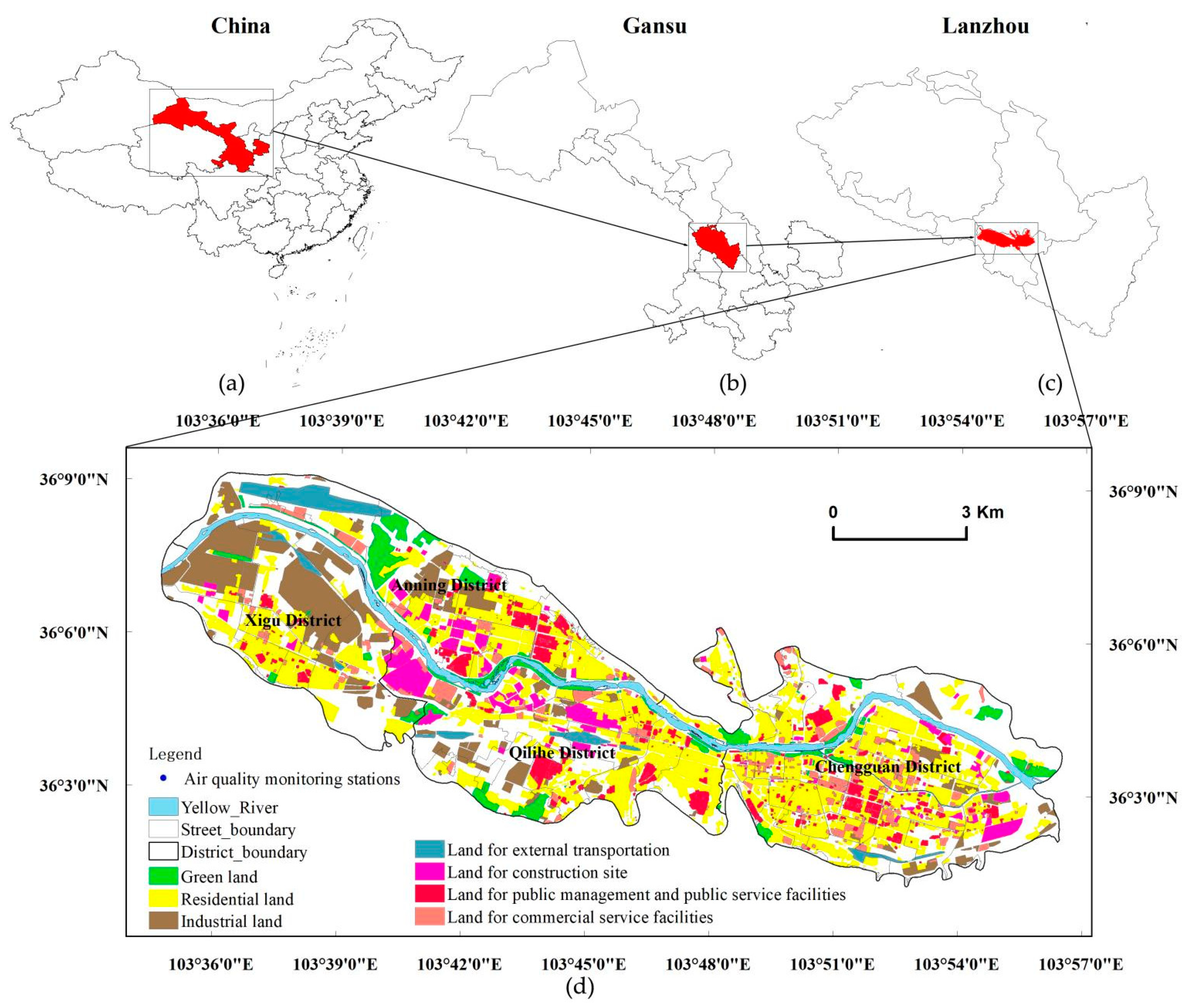
2.1. Study Area

Lanzhou City is located at 35°34′–37°07′ N and 102°36′–104°34′ E (Figure 1). It has a typical continental climate with average annual rainfall of 327 mm, which is mainly concentrated from June to September. The central city of Lanzhou has high terrain in the west and low terrain in the east, with two mountains in the north and south. The Yellow River runs through the entire territory from west to east, connecting the Xigu, Qilihe-Anning, and Chengguan Basins. The special river valley landform conditions and the meteorological and climatic conditions, in which the proportion of quiet windy days per year reaches more than 50%, make it difficult for air pollutants to spread; as a result, Lanzhou was classified as a severely polluted city by the World Health Organization [54]. As an important industrial base in Northwest China, Lanzhou has formed an industrial system dominated by oil refining, chemicals, electromechanics, metallurgy, military, energy, light and textile, and building materials after the construction of the First and Second Five-Year Plans and the Third Front. The industrial layout of the heavy petrochemical industry and the structure of coal-fired energy create mixed air pollution. With the launch of national air pollution prevention and control measures in 2012, the implementation of the Air Pollution Prevention and Control Plan in 2015, and the adjustment of the urban industrial structure, the urban air pollution situation has been significantly improved, with frequent occurrence of the “Lanzhou blue” phenomenon. Lanzhou City won a reform and progress award at the Paris Climate Conference in 2015.

2.2. Data Sources

2.2.1. Air Quality Data

We selected AQI to quantitatively describe and comprehensively reflect air quality status. The higher the index, the more serious the air pollution. The AQI data come from the mobile phone app of the public version of the Lanzhou Urban Atmospheric Environment Grid Monitoring System (http://sthjj.lanzhou.gov.cn/col/col4210/index.html (accessed on 31 December 2020)). We obtained the location information and AQI data of 479 air quality monitoring stations in the central urban area of Lanzhou from 1 January to 31 December 2020. Excluding data outside the study area and incomplete data, data from 340 air quality monitoring stations were obtained. We transformed the location information of the monitoring site into longitude and latitude coordinates in a data format that could be analyzed by ArcGIS software for later analysis. The study area and air quality monitoring stations are shown in Figure 1.

2.2.2. Urban Land Use Data

Most of the land use data in previous studies came from 30 m resolution remote sensing images. According to the Classification of Land Use Status (GB/T 21010-2017), land use has been subdivided into agricultural, water use, urban construction, unused land, etc. [8]. Previous studies went beyond the urban built-up area or took the urban area as a whole, which makes it difficult to reflect differences in land use within a city, and does not consider the coupled relationship between air quality and land use. According to the Urban and Rural Land Classification and Planning and Construction Land Standards (GB50137-2011), this paper subdivides urban construction land into green, residential, and industrial land, and land for external transportation, public management and public service facilities, and commercial service facilities. The emission of building dust is an important part of the dust source [55]. Therefore, we added additional land for construction sites. The land use data come from the current urban land use and planning maps in the Lanzhou City master plan.

2.2.3. Other Data

Urban air pollution sources include fixed and mobile sources. Fixed pollution sources include factories and heating boilers, and the mobile pollution source is motor vehicle exhaust [56]. For this study, we selected industrial enterprises above a designated size to characterize industrial pollution sources. The data come from the Chinese industrial enterprises database and the directory of industrial and commercial enterprises registered in Lanzhou City, Gansu Province. Heating boiler data come from the Lanzhou directory of heating service companies for 2019–2020. There are 138 industrial enterprises and 288 heating boilers in total. Traffic pollution is the main source of mobile pollution in cities. There are more vehicles in areas with dense road networks, producing more air pollutants [57]. We used road network density within a 1000 m buffer zone around the air quality monitoring sites to express traffic emissions [39]. Road network data come from OpenStreetMap (OSM) (www.openstreetmap.org (accessed on 12 March 2021)).

In this paper, the dependent variables are average AQI for the whole year, spring, summer, autumn, winter, heating period, and non-heating period, which are labeled as Y1, Y2, Y3, Y4, Y5, Y6, and Y7, respectively. The independent variable is the land use factor within a 1000 m buffer zone around each air quality monitoring station (

Table 1. Descriptive statistics of variables.

Factors		Variables (1000 m Buffer Zone)	Min	Max	Mean	Std. Dev.	VIF
X1	Heating emissions	Number of heating stations (pieces)	0	48	8.31	9	1.78
X2	Industrial emissions	Industrial enterprises above designated size (pieces)	0	14	2.28	2.34	1.33
X3	Traffic emissions	Road network density (km/km2)	0.62	8.22	4.1	1.73	2.16
X4	Industrial land	Proportion of industrial land	0	0.73	0.07	0.11	1.87
X5	Land for construction sites	Proportion of land used for construction sites	0	0.58	0.04	0.08	1.19
X6	Land for public management and public service facilities	Proportion of land for public management and public service facilities	0	0.36	0.08	0.07	1.23
X7	Green land	Proportion of green land	0	0.35	0.03	0.05	1.32
X8	Residential land	Proportion of residential land	0.02	0.86	0.51	0.18	1.85
X9	Land for commercial service facilities	Proportion of land for commercial service facilities	0	0.3	0.07	0.06	1.36
X10	Land for external transportation	Proportion of land for external transportation	0	0.31	0.01	0.03	1.29

). A total of seven regression models were constructed for the seven variables.

2.3. Research Methods

2.3.1. Correlation Analysis

The impact of land use on air quality has a scale effect [36]. The spatial scale is too large to identify differences in land use. Therefore, we first calculated that the maximum distance between the monitoring stations is 1971 m and the average distance is 323.49 m. Then, we built 5 buffer zones with a radius of 330, 500, 1000, 1500, and 2000 m. The Pearson correlation coefficient was used to investigate the correlation between air quality concentration and land use composition within these 5 buffer zones around the 340 monitoring stations. Its expression is as follows:

$$R_{xy}=\frac{{{\displaystyle \sum }}_{i=1}^n\left(x_i-\overline{x}\right)\left(y_i-\overline{y}\right)}{\surd {{\displaystyle \sum }}_{i=1}^n{\left(x_i-\overline{x}\right)}^2\surd {{\displaystyle \sum }}_{i=1}^n{\left(y_i-\overline{y}\right)}^2}$$

where n is the number of samples, $x_i$ is the observed value of point i corresponding to variable x, $y_i$ is the observed value of point i corresponding to variable y, $\overline{x}$ is the average of x samples, and $\overline{y}$ is the average of y. Rxy is the Pearson correlation coefficient, and its range is between −1 and 1. There is a negative relationship between two variables (x and y) when R_xy < 0 and a positive relationship when R_xy > 0. If the absolute value of R_xy is close to 1, that indicates a strong correlation between variables x and y. If the absolute value of R_xy is close to 0, then the correlation relationship is weak.

It is found that within 1000 m, the correlation coefficient between land use and air quality is high and the explanatory power is good (

Table 2. Results of Pearson correlation coefficient analysis.

	Variable	X1	X2	X3	X4	X5	X6	X7	X8	X9	X10
330 m buffer zone	Y1	−0.116 *	0.187 **	0.111 *	0.141 **	0.018	0.011	−0.123 *	−0.047	0.008	−0.04
	Y2	−0.201 **	0.173 **	0.142 **	0.161 **	0.038	0.033	−0.184 **	−0.092	0.029	−0.058
	Y3	−0.241 **	0.162 **	0.232 **	0.197 **	0.03	0.046	−0.297 **	−0.069	0.044	−0.05
	Y4	0.102	0.079	−0.049	0.006	0.003	0.023	0.073	0.034	−0.047	0.064
	Y5	0.145 **	0.091	0.129 *	0.043	−0.035	−0.055	0.221 **	0.027	−0.086	−0.039
	Y6	0.091	0.122 *	0.067	0.005	−0.004	−0.033	−0.125 *	0.013	−0.057	−0.032
	Y7	−0.203 **	0.176 **	0.183 **	0.181 **	0.026	0.032	−0.231 **	−0.069	0.022	−0.035
500 m buffer zone	Y1	−0.124 *	0.321 **	0.025	0.221 **	0.084	0.01	−0.171 **	−0.003	−0.058	0.016
	Y2	−0.208 **	0.332 **	0.037	0.265 **	0.129 *	0.008	−0.231 **	−0.077	−0.035	−0.04
	Y3	−0.295 **	0.244 **	0.153 **	0.233 **	0.138 *	0.053	−0.335 **	−0.089	0.045	0.004
	Y4	0.133 *	0.137 *	0.130 *	0.051	−0.048	0.016	0.071	0.142 **	−0.157 **	0.126 *
	Y5	0.191 **	0.168 **	0.260 **	0.009	−0.053	−0.059	0.184 **	0.097	−0.092	0.018
	Y6	0.134 *	0.245 **	0.198 **	0.1	−0.018	−0.04	−0.09	0.066	−0.126 *	0.034
	Y7	−0.237 **	0.281 **	0.079	0.232 **	0.119 *	0.036	−0.273 **	−0.041	−0.004	0.002
1000 m buffer zone	Y1	−0.281 **	0.588 **	0.151 **	0.536 **	0.069	0.199 **	−0.317 **	−0.096	0.081	0.321 **
	Y2	−0.393 **	0.579 **	0.208 **	0.559 **	0.167 **	0.218 **	−0.375 **	0.174 **	0.043	0.360 **
	Y3	−0.499 **	0.496 **	0.389 **	0.500 **	0.260 **	0.222 **	−0.504 **	0.288 **	0.180 **	0.327 **
	Y4	0.170 **	0.293 **	−0.049	0.164 **	−0.088	0.014	−0.203 **	0.120 *	−0.294 **	0.068
	Y5	0.258 **	0.225 **	0.329 **	0.181 **	−0.302 **	−0.058	0.141 **	−0.245 **	−0.355 **	0.062
	Y6	0.180 **	0.369 **	0.174 **	0.306 **	−0.197 **	−0.097	−0.018	0.154 **	−0.306 **	0.161 **
	Y7	−0.428 **	0.560 **	0.295 **	0.528 **	0.201 **	0.205 **	−0.433 **	0.212 **	0.066	0.328 **
1500 m buffer zone	Y1	−0.207 **	0.430 **	0.079	0.329 **	0.075	0.102	−0.284 **	−0.011	−0.068	0.052
	Y2	−0.318 **	0.424 **	0.141 **	0.370 **	0.141 **	0.126 *	−0.332 **	0.065	−0.037	0.006
	Y3	−0.428 **	0.317 **	0.317 **	0.330 **	0.205 **	0.108 *	−0.439 **	−0.167 **	0.046	0.147 **
	Y4	0.138 *	0.181 **	−0.083	0.096	−0.042	0.047	−0.005	0.161 **	−0.161 **	0.098
	Y5	0.253 **	0.136 **	0.345 **	0.103	−0.204 **	−0.059	0.132 *	−0.242 **	−0.167 **	0.150 **
	Y6	0.146 **	0.265 **	0.210 **	0.113 **	−0.119 *	−0.062	0.033	0.188 **	−0.144 **	0.024
	Y7	−0.353 **	0.386 **	0.221 **	0.340 **	0.166 **	0.099	−0.380 **	0.091	−0.007	0.081
2000 m buffer zone	Y1	−0.133 *	0.306 **	0.002	0.172 **	0.067	0.05	−0.126 *	0.018	−0.033	0.058
	Y2	−0.241 **	0.325 **	0.061	0.124 **	0.116 *	0.067	−0.176 **	−0.08	0.006	0.013
	Y3	−0.350 **	0.221 **	0.218 **	0.120 **	0.152 **	0.025	−0.285 **	−0.112 *	0.09	0.119 *
	Y4	0.106	0.180 **	−0.108 *	0.101	−0.033	0.028	0.065	0.089	−0.111 *	0.087
	Y5	0.238 **	0.185 **	0.323 **	0.075	−0.125 *	−0.073	0.186 *	−0.134 *	−0.120 *	0.107 *
	Y6	0.110 *	0.175 **	0.223 **	0.006	−0.069	−0.06	0.006	0.075	−0.138 *	0.04
	Y7	−0.274 **	0.276 **	0.129 *	0.191 **	0.127 *	0.032	−0.131 *	0.066	0.034	0.099

** At the 0.01 level (two-tailed), the correlation is significant, * At the 0.05 level (two-tailed), the correlation is significant.

). In subsequent research, the 1000 m buffer zone around the monitoring station was used as a spatial scale to explore the relationship between air quality and land use.

2.3.2. Inverse Distance Weight (IDW)

It can be seen from Figure 1 that the distribution of air quality monitoring points in the downtown area of Lanzhou cannot cover the entire city. This research attempts to analyze the temporal and spatial characteristics of the city’s air quality through spatial interpolation.

Spatial interpolation is a method of estimating unknown points through known points. It is derived from the first law of geography, that is, the closer the points in space, the more similar their characteristics. It has been widely used in many fields, such as environment, soil, and digital terrain analysis. Commonly used spatial interpolation methods include inverse distance weight (IDW), kriging, spline, trend surface, and natural neighbor [58]. In order to accurately simulate the time and space distribution of air quality in the city, these four methods were used to obtain the city’s AQI data, and then the interpolation results were cross-validated, and the best fit was compared. R² and root mean square error (RMSE) were used to determine the optimal interpolation method. The calculation method is as follows:

$$R^2=\frac{\sum {\left(\widehat{y}-\overline{y}\right)}^2}{\sum y^2}$$

$$RMSE=\sqrt{\frac{{{\displaystyle \sum }}_i^n{\left(\widehat{y}-\overline{y}\right)}^2}{n}}$$

where n is the number of test sample points, y is the actual measured value corresponding to the test interpolation point, $\widehat{y}$ is the estimated value corresponding to the test interpolation point, and $\overline{y}$ is the mean AQI value of the test interpolation point. R² represents the degree of fit between the interpolation result and the measured value; the closer to 1, the better the interpolation effect. RMSE represents the degree of deviation between the interpolation result and the measured value; the smaller the value, the higher the interpolation accuracy.

The calculation results (

Table 3. Comparison of interpolation methods.

	IDW	Kriging	Trend Surface	Spline	Natural Neighbor
R2	0.985383874	0.977285623	0.621729574	0.828676546	0.961090602
RMSE	2.914003447	2.902368713	2.488706625	2.827320784	2.927091981

) show that the average R² of IDW is the highest and the RMSE is the smallest. This paper selected IDW to study the spatial distribution of AQI.

When the set of points is dense enough to capture the extent of local surface variation needed for the analysis, IDW is used [58]. IDW interpolation has the advantages of a simple principle, convenient calculation, and conformity to the first law of geography. It is widely used in research of air quality spatial distribution characteristics [59]. IDW takes the distance between the interpolation points and the sample points as the weighted average; the closer the sample points to the interpolation points, the greater the weight given by the sample points [58]. It can model various scales when predicting air quality, which can reduce the uncertainty of prediction in exposure assessment and is more reliable than kriging.

Let a series of discrete points be distributed on the plane whose coordinates and values are called Xi, Yi, Zi (i = 1, 2, …, n); then, the value of Z points can be obtained by weighted distance. According to the value of the surrounding discrete points, the value of the Z point is calculated by the distance weighted value. Its expression is as follows:

$$Z_0=\left[{\displaystyle \sum }_{i=1}^n\frac{Z_i}{d_i^k}\right]/\left[{\displaystyle \sum }_{i=1}^n\frac{1}{d_i^k}\right]$$

where $Z_0$ is the estimated value of point 0, $Z_i$ is the value of control point i, d_i is the distance between control point i and point 0, n is the number of control points used in the estimation, and k is the specified power. In this paper, the inverse distance weighted difference method provided by ArcGIS10.2 was used to obtain all AQI values in the study area.

2.3.3. Getis-Ord Gi*

IDW can show the spatial distribution of AQI, but it has no statistical significance. Therefore, an optimized hot spot analysis was performed to show the statistical significance of highly polluted areas.

Getis-Ord Gi* is an effective method for calculating spatial autocorrelation that was proposed by mathematicians Getis and Ord in 1992. It is a statistic that identifies the specific locations of statistically significant point clusters with high data point density in the vicinity of a given point. Features with a high value density may not represent a statistically significant hot spot, and a hot spot can be determined if a feature with high value density is surrounded by other features with high values as well. It can qualitatively determine spatial hot or cold spot areas on a local scale and increase the confidence probability. Its expression is as follows [60]:

$$G_i^{*}=\frac{{{\displaystyle \sum }}_{j=1}^n{W}_{i,j\mathcal{X}j}-\overline{X}{{\displaystyle \sum }}_{j=1}^n{w}_{i,j}}{{{\displaystyle \sum }}_j^n{W}_{i,j\mathcal{X}j}}$$

where W_i,j is the spatial weight between feature i and j. A positive $G_i^{*}$ value shows that high values cluster around i; hence, the region is considered a hot spot. A negative value of $G_i^{*}$ shows that low values cluster around i; hence, the region is considered a cold spot. Since the monitoring stations provide point data, this paper uses the inverse distance weighted difference method provided by ArcGIS 10.2 to obtain all AQI values in the study area, then constructs a 1000 × 1000 m fishing net using the extraction and analysis tool in ArcGIS to obtain the AQI value of each fishing net center, and then uses the spatial joint tool in the Overlay toolset to connect the point data to the fishing net data. Then, the 1000 × 1000 m fishing net is taken as the spatial scale for Getis-Ord Gi* visualization.

2.3.4. Negative Binomial Regression Model

Regression models such as ordinary linear regression, Poisson regression, negative binomial regression, and zero inflation models are usually used to analyze data where the dependent variable is numerical, and ordinary least squares (OLS) is used when the relationship between them is linear and assumptions are observed. The assumptions of linear regression modeling include normality, independence, homoscedasticity of errors, exclusion of spatial autocorrelation, and multicollinearity [61]. When the dependent variable has a large number of zero values, the zero-inflated Poisson regression model (ZIP) [62] is useful. The Poisson distribution assumes that the expected and variance values are equal [63], but this is not always true, causing dispersion of data when the variance is higher than average, such as in studies linking air quality. When over-dispersion happens, one way to estimate its parameter is to use negative binomial distribution [64]. The negative binomial regression model is a continuous mixed Poisson distribution [65] that allows the Poisson mean to follow the y distribution, and its expression is:

$$\begin{array}{l}\mathrm{Pr}(Y=y)=\frac{\Gamma (y+\tau )}{y!\Gamma (\tau )}{\left(\frac{\tau }{\lambda +\tau }\right)}^{\tau }{\left(\frac{\lambda }{\lambda +\tau }\right)}^y\\ y=0,1,\dots ; \lambda , \lambda >0\\ \lambda =E(Y)\end{array}$$

where τ is the fuzzy parameter, and Y is the dependent variable, namely air quality, and the variance of Y is λ + λ²/τ. When τ tends to infinity, the negative binomial is close to the Poisson distribution. The negative binomial distribution has a very simple property: the variance is greater than the mean. This paper uses a negative binomial regression model to explore the relationship between urban air quality and land use.

3. Results

3.1. Spatiotemporal Characteristics of Urban Air Quality

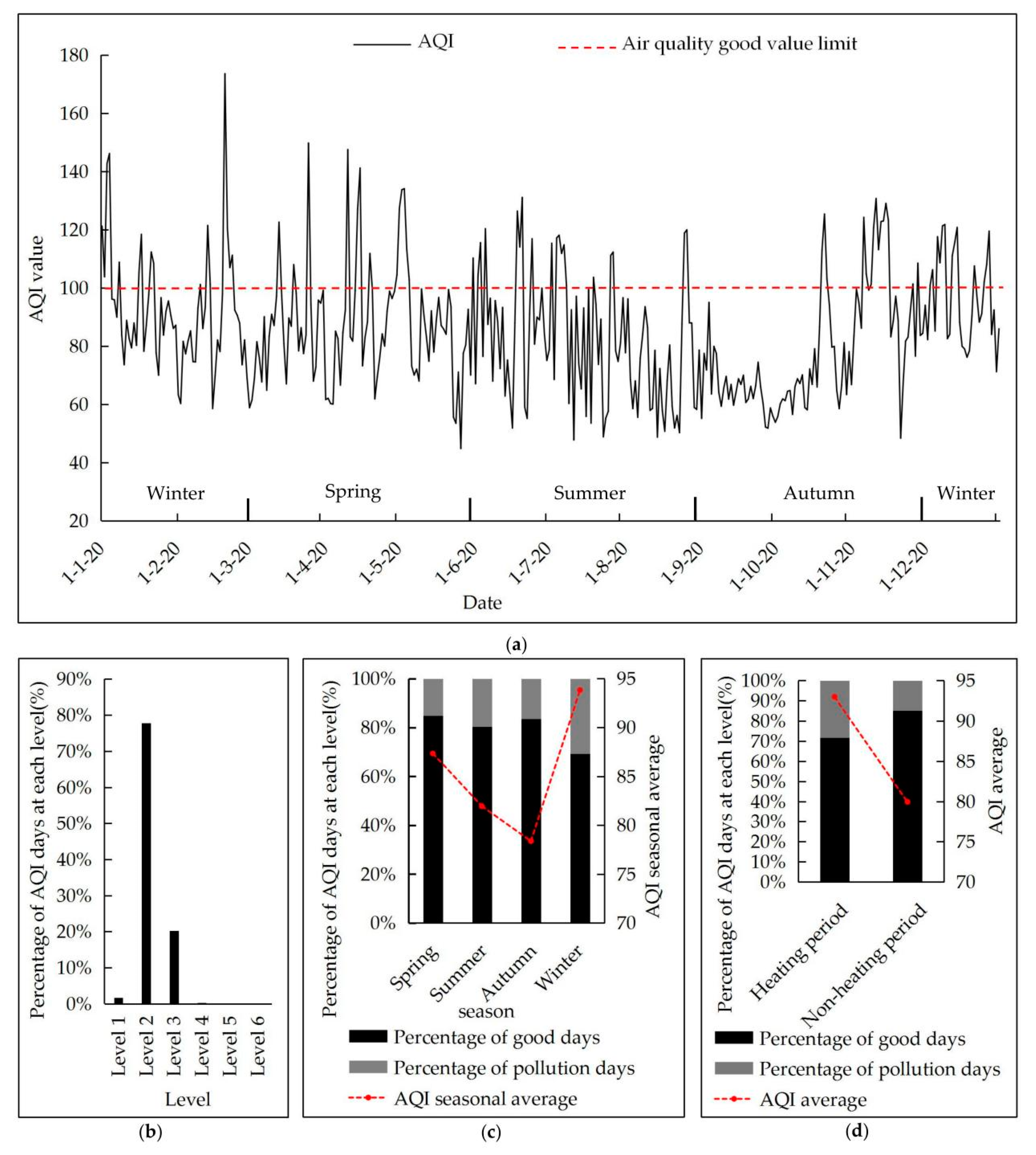
3.1.1. Temporal Distribution Characteristics

The annual AQI is represented by the continuous “valley–peak” interphase distribution characteristics of “low pollution–pollution peak–low pollution” (Figure 2a). The daily average of AQI fluctuated between 45 and 174, and the annual average was 85. There were 6 excellent days, 285 good days, 74 lightly polluted days, and 1 moderately polluted day. There was a total of 75 polluted days and 291 good days. The rate of excellent and good days was 79.5%, indicating that the air quality in Lanzhou was good.

We divided the year into four seasons, with March to May as spring, June to August as summer, September to November as autumn, and December to February as winter. In terms of the seasonal distribution of AQI (Figure 2c), the pollution degree was in the order of winter > spring > summer > autumn, but in terms of the rate of good air quality, it was in the order of winter > spring > autumn > summer. The air quality in summer and autumn was better than in winter and spring, showing the characteristics of a V-shaped change, and the seasonal average AQI value fluctuated between 74 and 96.

From the beginning of spring, the air quality slowly decreased to its lowest value in autumn and then rose rapidly to its highest value in winter. In spring, air quality was dominated by good days and light pollution, with a rate of excellent and good days of 84.78%. In summer, the number of good days with light pollution gradually increased and the number of good days gradually decreased, with a rate of excellent and good days of 80.43%. In autumn, atmospheric convection was strong and pollutants were diffuse, occurring relatively quickly, with significant precipitation, and the city’s air quality was the best, with a rate of excellent and good days of 83.52%. In winter, the city’s air quality was the worst, with a rate of excellent and good days of only 69.23% and a pollution rate of 30.77%.

The fundamental reason lies in the atmospheric circulation and heating in winter. Northwest wind prevails in Lanzhou in spring. There is much dusty weather, the concentration of particulate matter obviously increases, precipitation and relative humidity are low, and there is more dust and floating dust on the surface. The superposition of the two causes 40% of air pollution in spring [54,57]. In summer and autumn, affected by the East Asian and South Asian monsoons, the atmosphere has good diffusion conditions, which is conducive to the dilution and diffusion of pollutants. Rainfall increases, vegetation coverage significantly increases, and dust from roads and construction is suppressed. In winter, there is little precipitation, dry climate, dry vegetation, stable atmospheric stratification, severe temperature inversion, and poor conditions for dilution and diffusion of pollutants [66], and the entire city enters a long heating period, so winter pollution is the most serious. From the perspective of changes in the heating and non-heating period (Figure 2d), air quality during the heating period is poor and the pollution rate reaches 27%, and air quality during the non-heating period is better. This is consistent with research conclusions in Balıkesir, Turkey, and in the Rhine–Ruhr area of Germany [67,68].

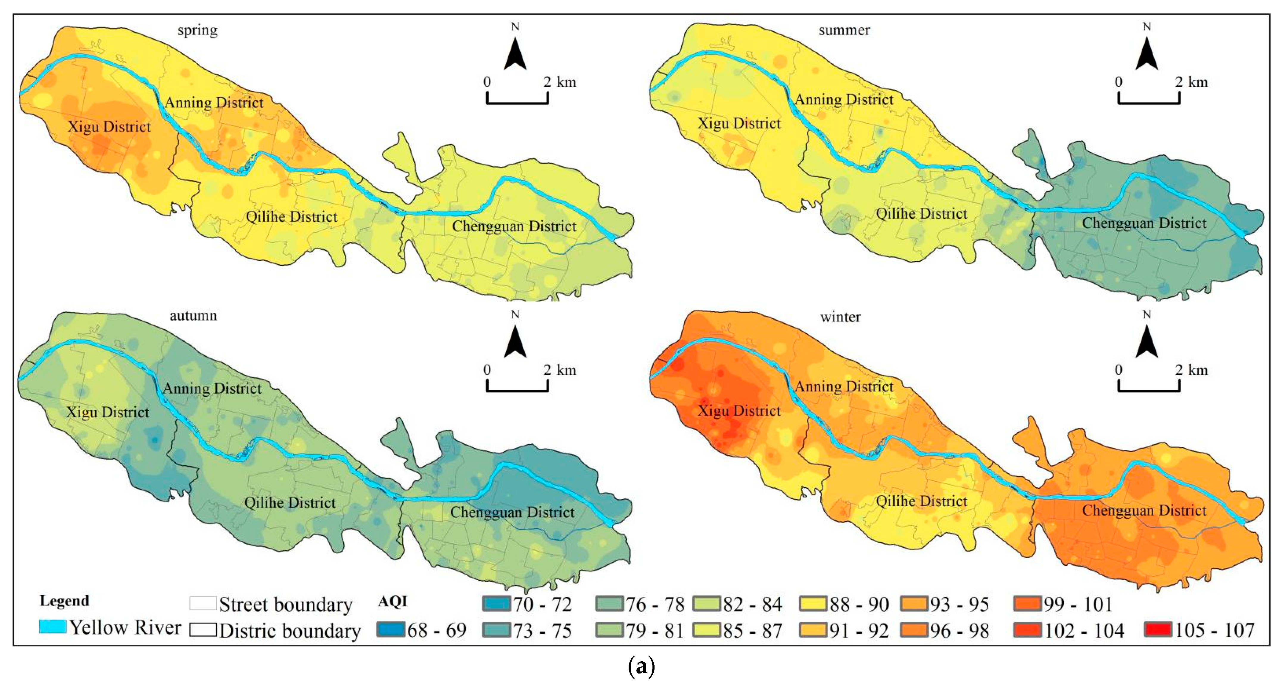
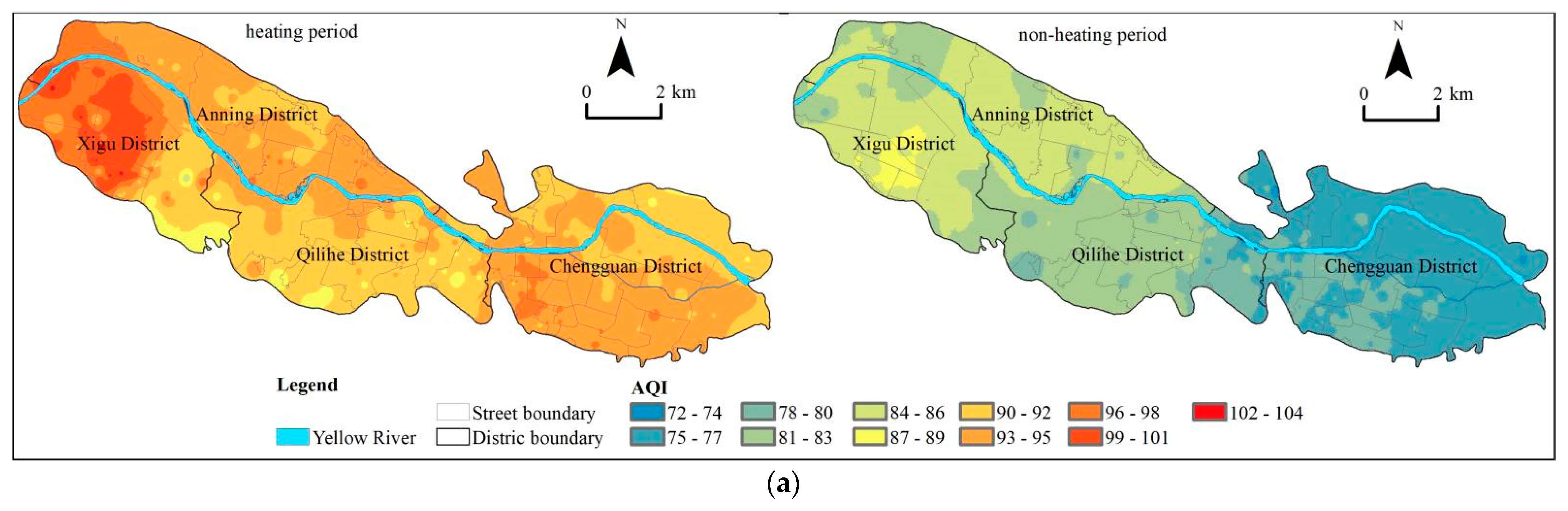
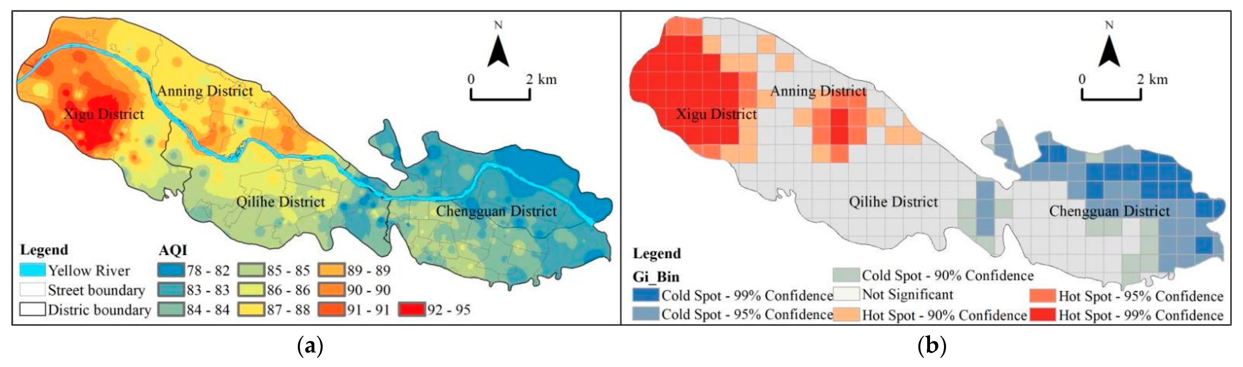
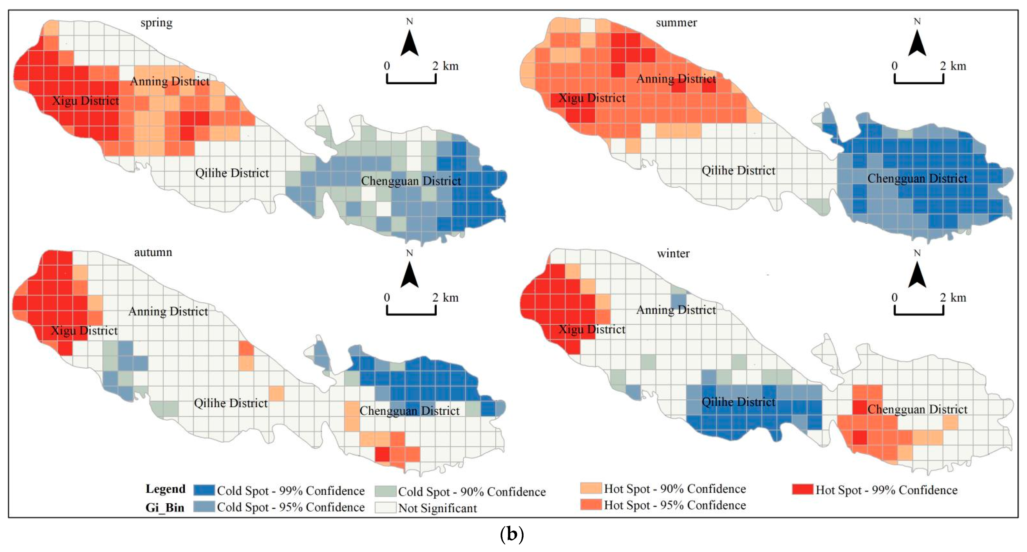
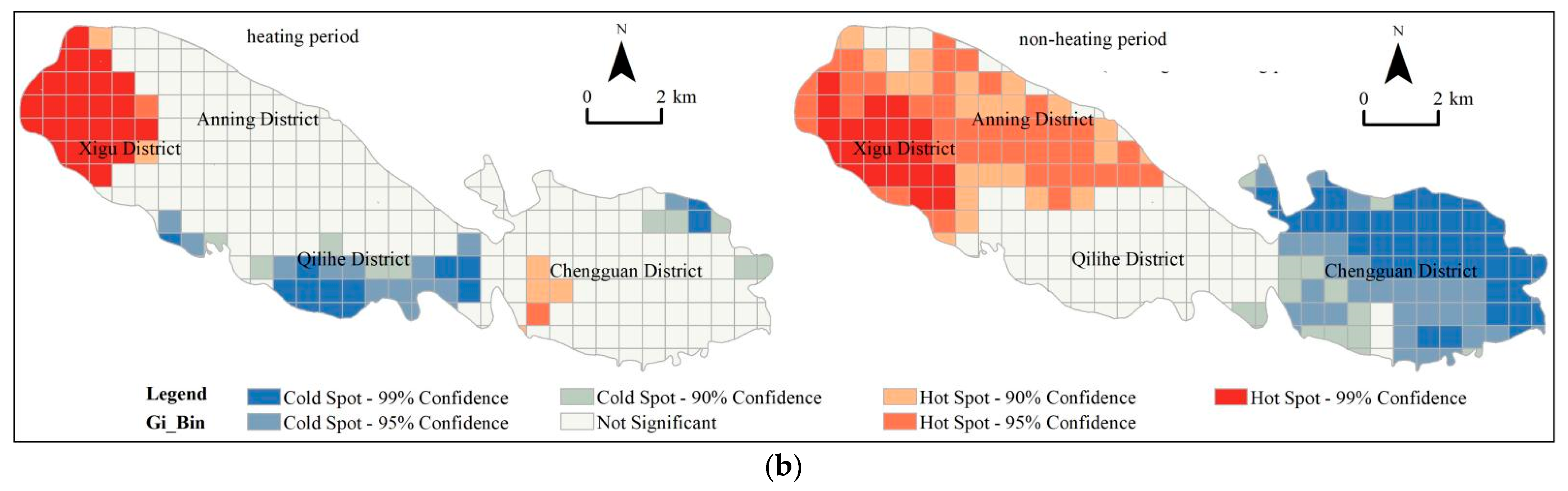
3.1.2. Spatial Clustering Features

AQI has obvious differentiation in space. In general, the degree of air pollution showed characteristics of heaviness in the west and lightness in the east, in the order of Xigu District > Anning District > Qilihe District > Chengguan District (Figure 3a). Hot spots are mainly concentrated in Xigu and Anning and cold spots mainly in Chengguan, while the agglomeration characteristics of Qilihe District are not significant (Figure 3b). This may be related to urban functions, land use structure, industrial enterprise layout, and energy consumption intensity. Xigu District forms the city’s pollution core, dominated by Xiliugou, Sijiqing, Xigucheng, and Fuli Road Streets, with an AQI over 90. The main reason is that Xigu is the most important industrial area in Lanzhou, with nearly 50% of the land used for industry, and there are heavy and chemical industries such as Lanzhou Xigu Thermal Power Plant, Lanzhou Petrochemical Company, Lanzhou Petrochemical Company of PetroChina, Fanping Power Plant, Lanzhou Gas Plant, and so on. Most of these enterprises are in the thermal power, crude oil smelting, and petrochemical industries. Their emission of pollutants is in excess of the city’s industrial emissions of 50%.

Anning is the cultural district of Lanzhou City, as well as the distribution area of the instrument and high-tech industries, so a number of point pollution cores have formed: Shilidian, Yintan Road, Xilu, and Shajingyi Streets. The AQI of the whole region is over 85, and the pollution degree decreases from the north bank of the Yellow River to Renshou Mountain. The main reason is that Anning is close to Xigu and the area along the river is susceptible to industrial pollution. The high AQI of Shilidian Street in the east is related to the waste gas emissions of the sewage treatment plant.

Qilihe District is bounded by Xihu Street, where pollution is heavy in the west and light in the east, high in the north (south bank of the Yellow River), and low in the south. Xiuchuan, Gongjiawan, Pengjiaping, and Jingangcheng are four low-pollution areas. Qilihe undertakes the city’s commercial, living, and productive services and other functions and is also the most important construction and development zone in the built-up area. There are many construction sites in the “three beaches”, the Matan, Cuijiadandatan, and Yingmentan areas. Dust has a certain amount of impact on air quality. The air quality in Chengguan District is better, and the AQI is below 85. The main reason is that Chengguan is the city’s administrative office and commercial area and is located in the upwind direction with fewer pollution sources (especially industrial sources).

Air pollution forms an obvious spatial process of clustering–diffusion with seasonal changes (Figure 4a). The hot spot in spring and summer is Xigu District, and the cold spot in Anning is Chengguan District. Great changes take place in the hot spot areas in autumn and winter. The hot spot area in autumn is mainly concentrated in Xigu District and the central areas of Qilihe and Chengguan Districts, while the cold spot area is mainly concentrated in the mountainous part of Qilihe and along the river in the northern part of Chengguan. In winter, two hot spots are formed in Xigu and Chengguan, and Qilihe is a cold spot area (Figure 4b). In the spring, the AQI of the whole city is between 80 and 97.

Spatially, an industrial pollution area centered on Xigu District and an area around the central business district of Datan and Peili Square in Anning–Yingmentan–Qilihe District have formed. For lightly polluted centers, the AQI is above 90. The Anning central business district and the “Santan” area have been key construction areas in Lanzhou in recent years, with a distribution of many construction sites, and construction dust has made these areas highly polluted. The AQI of the eastern part of Qili River and Chengguan District is basically between 82 and 90, and the pollution level is heavy in the west and light in the east. In summer, the city’s AQI is between 69 and 92. The low AQI area expands, and the high pollution area further shrinks in Xigu and Anning. The AQI is greater than 90.

Lightly polluted areas have formed in Anning District, such as Shajingyi, the central business district, and sewage treatment plants. Xiuchuan, Pengjiaping, and Xihu Streets in Qilihe District have even reached excellent grades. The whole area of Chengguan District is of excellent grade, with AQI below 80, and only light pollution occurs in the railway station, Yanchangbao, and Dongfanghong Square. In autumn, the city’s AQI is between 64 and 91, with only slight pollution in the surrounding areas of Lanzhou Xigu Thermal Power Plant, Lanzhou Petrochemical Company, and Anning District Sewage Treatment Plant. In winter, the city’s AQI is between 81 and 104.

Two moderately polluted areas, Xigu District with mainly industrial emissions and Chengguan District with mainly heating emissions, have formed, with an AQI of over 95. A surface pollution area formed in Chengguan dominated by Zhangye Road, Guangwumen, Jiuquan Road, Gaolan Road, Wuquan, Railway East Village, Railway West Village, and other streets. The main reason is that 56.5% of heating stations are gathered in Chengguan. Boilers emit large amounts of dust and SO₂, forming low-altitude non-point-source pollution [69]. The air quality in Anning and Qilihe Districts is relatively good, and the AQI is basically between 90 and 95. Even marginal areas have low values, such as Chenping Street in the east of Xigu and Pengjiaping Town in Qilihe.

The heating period in Lanzhou is from the beginning of November to the end of March, and the non-heating period is from the beginning of April to the end of October. It can be seen from Figure 5 that air pollution during the heating period is obviously more serious than during the non-heating period. The AQI of the whole city during the heating period is between 82 and 104. The AQI of the whole city during the non-heating period is between 70 and 88. During the heating period, two pollution cores are formed in Xigu and Chengguan Districts (Figure 5). Anning District is also a heavily polluted area in the city due to the prevailing wind direction [52]. It is shown that the spatial variation of air pollutants is affected not only by local emission but also by meteorological conditions (such as wind), which cause secondary pollution near the emission source [36]. In terms of spatial agglomeration, the core areas of Xigu and Chengguan Districts are hot spots, the mountainous area in the south of Qilihe District is a cold spot area, and the agglomeration of Anning District is nonsignificant. The air quality of Lanzhou is gradually stable during the non-heating period, and the air pollution is heavy in the west and light in the east. The spatial agglomeration model shows that the stable hot spots of pollution are Xigu and Anning Districts, the cold spot is Chengguan District, and the spatial agglomeration characteristics of Qilihe District are not significant.

3.2. Relationship between Urban Air Quality and Land Use

Using SPSS software to test the normality of each dependent variable to determine whether it was discrete data (

Table 4. Normality test of data.

Variable	Mean	Variance	Wa	p
Y1	86	8.529	0.965	0
Y2	88	13.895	0.950	0
Y3	82	36.377	0.889	0
Y4	79	9.144	0.986	0.002
Y5	94	13.544	0.994	0.222
Y6	93	9.113	0.960	0
Y7	80	14.704	0.950	0

Note: Normality tested by Shapiro–Wilk test.

), we found that the significance level of Y1, Y2, Y3, Y4, Y6, and Y7 was less than 0.05, in a discrete distribution state. Only Y5 had a significance greater than 0.05 (0.222). The main reason is that Lanzhou has frequent static winds in winter, a high inversion rate of 99% [69], and poor diffusion conditions, resulting in seemingly distributed air quality data. Air quality is discrete data, and none of the data had a value less than 0. This paper used a negative binomial regression model for regression analysis.

In order to improve the simulation accuracy of the model, it is necessary to check the collinearity of the respective variables. The analysis results (Table 4) show that the VIF of each variable is less than 3 and is far less than the critical value of 10, which indicates that the model has no multicollinearity problem and can be used for negative binomial regression analysis.

The negative binomial regression model analysis results (

Table 5. Negative binomial model results.

Variables	M1	M2	M3	M4	M5	M6	M7
X1	−0.00019816 (−0.92)	−0.0007814 *** (−3.51)	−0.00173062 *** (−4.47)	0.00107369 *** (3.32)	0.00053515 * (2.19)	0.00057556 ** (2.72)	−0.00086096 ** (−3.15)
X2	0.00429904 *** (5.19)	0.00540908 *** (5.48)	0.0066031 *** (4.59)	0.00310282 *** (3.84)	0.00224721 * (1.99)	.00296906 ** (3.29)	0.00540177 *** (5.26)
X3	0.00414971 *** (3.31)	0.00534804 *** (3.47)	0.00410567 (1.70)	−0.00022114 (−0.14)	0.00664185 *** (4.04)	0.00421788 ** (3.18)	0.00407687 * (2.50)
X4	0.18057696 *** (4.76)	0.12480744 ** (2.63)	0.45315445 *** (5.19)	0.19876456 *** (3.53)	−0.02347487 (−0.54)	0.07403405 (1.91)	0.26899138 *** (4.73)
X5	0.05019174 * (2.42)	0.06809959 * (2.55)	0.16797907 *** (4.09)	−0.02767476 (1.05)	−0.05262646 (−1.82)	−0.00819725 (−0.36)	0.09824626 *** (3.63)
X6	0.02209244 (0.95 )	0.01899393 (0.65)	0.13869561 ** (3.07)	0.02586483 (0.96)	−0.08079757 ** (−2.87)	−0.03109436 (−1.41)	0.06620023 * (2.18)
X7	−0.1662874 *** (−6.95)	−0.21372142 *** (−7.27)	−0.47167738 *** (−10.63)	−0.01679669 (−0.51)	0.01593301 (0.51)	−0.03059924 (−1.19)	−0.27981642 *** (−8.95)
X8	0.03085474 ** (2.66)	0.02762988 * (2.00)	0.09474067 *** (3.89)	0.01392373 (0.96)	−0.00599751 (−0.43)	0.00047415 (0.04)	0.05649607 *** (3.54)
X9	0.02789775 (0.67)	0.03558245 (0.76)	0.24589958 ** (3.29)	−0.08055354 (−1.84)	−0.08187814 (−1.52)	−0.06773554 (−1.57)	0.10692261 * (2.06)
X10	0.06640575 *** (3.45)	0.07624238 *** (3.49)	0.12397266 *** (3.44)	0.02951012 (1.35)	0.03569024 (1.24)	0.0450457 (1.84)	0.08384093 *** (3.43)
_cons	4.4093038 *** (553.85)	4.4330281 *** (466.38)	4.3374985 *** (233.47)	4.3384706 *** (404.55)	4.545 *** (474.31)	4.5089679 *** (552.08)	4.3316371 *** (366.43)
N	340	340	340	340	340	340	340

t statistics shown in parentheses. * p < 0.1, ** p < 0.05, *** p < 0.01.

) show that all negative binomial regressions were statistically significant (p < 0.01) with high fitting precision.

The results of the annual regression model show that air quality is negatively correlated with green land and positively correlated with industrial emissions, traffic emissions, industrial land, and land for external transportation at the 0.01 significance level and residential land at the 0.05 significance level. It is positively correlated with land for construction sites at the 0.1 significance level, and the degree of impact shows the order of industrial land > land for external transportation > traffic emissions > heating emissions > residential land > land for construction sites. In spring, air quality is negatively correlated with heating emissions and green land at the 0.01 significance level, and the impact of green land is greater than heating emissions. It is positively correlated with industrial emissions, traffic emissions, and land for external transportation at the 0.01 significance level. It is positively correlated with industrial land at the 0.05 significance level. There is a positive correlation with land for construction sites and residential land at the 0.1 significance level, and the degree of influence shows the order of land for external transportation > industrial emissions > traffic emissions > industrial land > land for construction sites > residential land.

In summer, air quality is negatively correlated with heating emissions and green land at the 0.01 significance level, and the impact of green land is greater than heating emissions. It is positively correlated with industrial emissions, industrial land, land for construction sites, residential land, and land for external transportation at the 0.01 significance level. At the 0.05 significance level, it is positively correlated with land for public management and public service facilities, and land for commercial service facilities, and the degree of impact shows the order of industrial land > land for construction sites > land for external transportation > residential land > industrial emissions > land for public management and public service facilities > land for commercial service facilities.

In autumn, air quality is positively correlated with heating emissions, industrial emissions, and industrial land at the 0.01 significance level, and the degree of influence shows the order of industrial land > industrial emissions > heating emissions. In winter, air quality is positively correlated with traffic emissions at the 0.01 significance level, and positively correlated with heating emissions and industrial emissions and negatively correlated with land for public management and public service facilities at the 0.1 significance level. The degree of impact shows the order of traffic emissions > industrial emissions > heating emissions. During the heating period, air quality is positively correlated with heating, industrial, and traffic emissions at the 0.05 significance level, and the degree of influence shows the order of traffic emissions > industrial emissions > heating emissions. During the non-heating period, air quality is negatively correlated with green land and positively correlated with industrial emissions, industrial land, land for construction sites, residential land, and land for external transportation at the 0.01 significance level. There is a negative correlation with heating emissions at the 0.05 significance level. There is a positive correlation with traffic emissions, land for public management and public service facilities, and land for commercial service facilities at the 0.1 significance level, and the degree of impact is in the order of industrial land > land for construction sites > land for external transportation > residential land > industrial emissions > land for commercial service facilities > land for public management and public service facilities > traffic emissions.

Overall, there is a close relationship between urban land use and air quality. Industrial activities, traffic pollution, and urban construction activities are the most important factors affecting urban air quality. Green space can reduce urban pollution. Industrial land has a serious impact on the quality of the air environment in terms of area and spatial distribution. As the “green lung” of the city, green land can adsorb and settle most air pollutants; the larger the green land, the better the air quality. The impact of land use on air quality has a seasonal effect and shows a certain time coupling with local social and economic activities. There is not a clear positive or negative correlation between all urban construction land and air quality. Land for public management and public service facilities has a positive correlation with air quality in summer and non-heating periods, and a negative correlation in winter, and there is no obvious mathematical relationship in other models. The land used for commercial service facilities only shows a positive correlation with air quality in summer and non-heating periods, and there is no obvious mathematical relationship in other models.

4. Discussion

Previous studies mostly obtained air quality data from five national air quality monitoring stations in Lanzhou [50,70]. Due to the lack of monitoring stations, it is difficult to truly and effectively describe the temporal and spatial evolution of air quality in the city [36]. There are some defects in the identification of polluted area inside the city [3]. In this study, AQI data from 340 air quality monitoring stations in Lanzhou were used to make up the deficiency of previous studies, which can clearly depict the spatiotemporal change law of air quality and identify high-pollution areas in the city. The modeling of the relationship between land use and air quality was mainly based on annual average air quality data, ignoring seasonal differences, and the research results show that construction land has a significant effect on urban air quality. There is no detailed classification of urban construction land, so this paper discusses the relationship between land use and air quality by using the refined land use data within the buffer zone of 1000 m around the air quality monitoring station. It is found that not all construction sites cause air pollution, and different types of land have different effects on air quality. The effect of land use on air quality also has seasonal differences under different model conditions, to a certain extent, and this conclusion extends the previous research and provides a practical case for micro-scale air quality distribution and its driving factors based on land use.

The study found that the rate of excellent and good air quality in Lanzhou reached 79.5%, which is consistent with the research conclusions of Sun, Ma, Guan, and others [46,49,50]. This is in line with the development trend of air quality in China [19], which cannot be separated from air pollution mitigation measures such as central heating, traffic restrictions, and street sprinkling [39]. In terms of time distribution, it has the characteristics of alternating high and low pollution and obvious seasonal changes throughout the year. Pollution in winter and spring is more serious than that in summer and autumn, which is consistent with the results of air quality research in China [12]. It is mainly affected by monsoon climate conditions and rain and heat conditions.

The air quality in Lanzhou City has spatial differentiation. Pollution in Xigu District is the most serious, which has been widely recognized by scholars [50,54,70]. The reason is that Xigu, as the largest heavy chemical industry zone in Lanzhou, has a large discharge of pollutants. In addition to the special geomorphic conditions of Lanzhou, air pollutants are not easily diffused, which leads to aggravation of pollution [70]. However, some scholars have found that there is no spatial heterogeneity in the air pollution in Lanzhou, which may be related to the research data [3]. Data from five national ambient air quality monitoring stations cannot identify differences in air quality within cities; a large quantity of data from monitoring stations is needed to clearly identify the differences in air quality within a city. The spatial distribution of air quality has seasonal differences, which is consistent with the conclusion of Shi [71]. However, Shi’s research did not identify where the seasonal differences in air quality within cities are reflected. The research in this paper found that in addition to the core of pollution in Xigu District, the air pollution in Lanzhou during the heating period is mainly concentrated in Chengguan District, which deepens previous research conclusions.

The spatial changes of air pollution in cities are closely related to land use. Different types of land use have different effects on air quality, which is consistent with the results of Jo’s research in Korea [35]. Industrial emissions, traffic emissions, industrial land, residential land, and land for external transportation cause air pollution, while green land can control air pollution, which is consistent with the previous yearly model [25,35,43]. Industrial and traffic emissions are the main causes of air pollution in Lanzhou [70]. Residential areas gather large numbers of people, and the high population density leads to deteriorated air quality [8].

The results of different seasonal models show that land for construction sites, heating emissions, and green land have seasonal effects on air quality. In winter and heating periods, only heating emissions, industrial emissions, and traffic emissions are positively correlated with the degree of air pollution, which is consistent with the research conclusions of Li. As the weather gets colder in winter, the inhibitory effect of vegetation on air pollutants gradually decreases from 16.6% in spring to 10.8% in winter. Traffic emissions are increased due to the weakened impact of green space [72], and mobile sources such as traffic cause more pollution than power generation and industry [73].

The secondary pollution in Lanzhou is relatively serious in winter, and the proportion of pollutants emitted by motor vehicles is relatively large [47]. Therefore, Lanzhou should adopt different air pollution prevention and control measures according to seasonal variations. The impact of land for public management and public service facilities and land for commercial service facilities on air quality is not clear, which is inconsistent with the research conclusions of Korean scholars [35]. These two studies found that commercial areas increase the degree of air pollution through real-time big data of smart sensors. The above inconsistent results may be caused by the accuracy of the data. Future studies can use smart sensors, big data, and other means to clearly describe the differences between the two.

5. Conclusions

5.1. Conclusions

Identifying the areas of poor air quality inside cities and their driving factors in terms of land use is a prerequisite and basis for effective air environmental governance, which is of great practical significance in order to promote sustainable development of the urban environment. This study contributes to the research on air quality and land use at the micro-scale by examining the changing laws of air quality and the relationship between urban land use and air quality based on data from 340 air quality monitoring stations.

The air quality in Lanzhou has the characteristics of temporal and spatial differentiation. Air quality varies throughout the year with high and low pollution, with obvious seasonal changes; summer and autumn are better than winter and spring, and air pollution is the most serious during the heating period. Air pollution presents a spatial pattern of heavy weight in the west and light weight in the east, characterized by the order of Xigu > Anning > Qilihe > Chengguan District.

The results of identifying hot and cold spots of air pollution show that the hot spots are mainly concentrated in Xigu and Anning and the cold spots are mainly concentrated in Chengguan. With seasonal changes, air pollution undergoes a process of “concentration–diffusion” in space. During the heating period, two air pollution hot spots form a perennial pollution core in Xigu and a heating core in Chengguan.

Different land use categories have different effects on air quality with regard to either the direction, magnitude, or seasonal scale effect of correlation. In general, industrial activities, traffic pollution, and urban construction activities are the most important factors affecting urban air quality. Green spaces can reduce urban pollution. The impact of land use on air quality has a seasonal effect.

The land use types are directly related to pollution emissions, which indirectly affects air quality. However, due to the influence of regional transmission and secondary conversion, future research should combine primary pollutants such as SO₂, NOx, dust (PM₁₀, PM_2.5), etc., and AQI to study their relationships with land use types. The AQI is a comprehensive representation of air pollution. Different pollutants have different relative contributions to the AQI in different seasons. For example, O₃ contributes significantly in summer, while PM contributes significantly in winter, which may lead to differences in the analysis of the spatial distribution of the AQI. Urban land use is static data, while air quality is dynamic data. Although studies have found seasonal differences in the impact of land use on air quality, using only one year of data might affect the stability of the conclusion. In the future, we need to acquire long-term dynamic data using new methods such as big data, machine learning, and intelligent sensors and rebuild the air–LUR model to fully study the coupled relationship between urban air quality and land use.

5.2. Policy Suggestions

Based on the analysis results of this study, different types of land use have different impacts on air quality. Similarly, the impact of land use on air quality under different model conditions has seasonal differences. Therefore, discussing methods to curb the deterioration of air quality does not mean that, in order to control the scale of urban construction land, it is necessary to subdivide the types of land, identify the types that affect air quality, optimize and adjust the land structure, and formulate sustainable urban land use policies to control air pollution. Specifically, the following should be addressed: (1) In urban planning, when optimizing the layout of urban functions, we should try to avoid the “spreading pie” type of urban space expansion, adopt a compact and intensive development model, alleviate the commuter traffic demand caused by the separation of work and residence, and implement public transportation. The priority strategy is to build a complete public transportation system and guide individuals to transfer to using it, thereby slowing the growth of motor vehicles, reducing traffic emissions, and improving air quality. (2) In urban land use planning, we should control the scale of industrial land, construction site land, and foreign-use land; gradually transfer industries in the central area of the city to the suburbs; reduce the proportion of industrial land; and use water bodies and land between polluting factories and other land. It is essential to protect and isolate open spaces to prevent industrial pollution. (3) In the planning of the urban green space system, we should increase the coverage of urban green space, cover areas with high concentrations of air pollutants, absorb urban air pollutants, improve air quality, and reduce the concentration of pollutants in the entire city. (4) We should strengthen the management of dust from urban roads and construction sites; promote an improved mechanized road cleaning rate, install atmospheric environment monitoring equipment and atomization and dust suppression devices on construction sites, and network with the environmental protection and housing construction departments to improve the management level of construction dust. (5) We should further optimize the energy structure, replace coal with clean energy, and reduce air pollution caused by coal burning during the heating period.

References

1. World Urbanization Prospects: The 2018 RevisionUnited Nations; Department of Economic and Social Affairs, Population Division: New York, NY, USA, 2018.
2. Tecer, L.H.; Tagil, S. Impact of Urbanization on Local Air Quality: Differences in Urban and Rural Areas of Balikesir, Turkey. Clean Soil Air Water 2014, 42, 1489–1499. [Google Scholar] [CrossRef]
3. Zhang, Y.; Li, M.; Bravo, M.A.; Jin, L.; Nori-Sarma, A.; Xu, Y.; Guan, D.; Wang, C.; Chen, M.; Wang, X.; et al. Air Quality in Lanzhou, a Major Industrial City in China: Characteristics of Air Pollution and Review of Existing Evidence from Air Pollution and Health Studies. Water Air Soil Pollut. 2014, 225, 2187. [Google Scholar] [CrossRef]
4. World Health Organization. Air Pollution. 2020. Available online: https://www.who.int/health-topics/air-pollution#tab=tab_2.2020-3-28 (accessed on 12 March 2021).
5. Yin, P.; Brauer, M.; Cohen, A.J.; Wang, H.; Li, J.; Burnett, R.T.; Stanaway, J.D.; Causey, K.; Larson, S.; Godwin, W.; et al. The effect of air pollution on deaths, disease burden, and life expectancy across China and its provinces, 1990–2017: An analysis for the Global Burden of Disease Study 2017. Lancet Planet. Health 2020, 4, 386–398. [Google Scholar] [CrossRef]
6. Abd Rani, N.L.; Azid, A.; Khalit, S.I.; Juahir, H.; Samsudin, M.S. Air Pollution Index Trend Analysis in Malaysia, 2010–15. Pol. J. Environ. Stud. 2018, 27, 801–807. [Google Scholar] [CrossRef]
7. Kanchan, K.; Gorai, A.K.; Goyal, P. A review on air quality indexing system. Asian J. Atmos. Environ. 2015, 9, 101–113. [Google Scholar] [CrossRef] [Green Version]
8. Tian, Y.; Jiang, Y.; Liu, Q.; Xu, D.; Zhao, S.; He, L.; Liu, H.; Xu, H. Temporal and spatial trends in air quality in Beijing. Landsc. Urban Plan. 2019, 185, 35–43. [Google Scholar] [CrossRef]
9. Hu, J.; Ying, Q.; Wang, Y.; Zhang, H. Characterizing multi-pollutant air pollution in China: Comparison of three air quality indices. Environ. Int. 2015, 84, 17–25. [Google Scholar] [CrossRef] [PubMed]
10. HJ 633-2012, Ambient Air Quality Index (AQI) Technical Regulations (Trial); China Environmental Science Press: Beijing, China, 2012.
11. Wang, Z.B.; Liang, L.W.; Wang, X.J. Spatio-temporal evolution patterns and influencing factors of PM2.5 in Chinese urban agglomerations. Acta Geogr. Sin. 2019, 74, 2614–2630. [Google Scholar]
12. Zhang, X.M.; Luo, S.; Li, X.M.; Li, Z.F.; Fan, Y.; Sun, J.W. Spatio-temporal Variation Features of Air Quality in China. Sci. Geogr. Sin. 2020, 40, 190–199. [Google Scholar]
13. Nurul, A.M.; Ling, O.H.L.; Omar, D. Urban Air Quality and Human Health Effects in Selangor, Malaysia. Procedia Soc. Behav. Sci. 2015, 170, 282–291. [Google Scholar]
14. Liu, Q.; Yang, Y.C.; Liu, H.Y. Spatiotemporal evolution characteristics of air pollution degree in 366 cities of China. Arid Land Geogr. 2020, 43, 820–830. [Google Scholar]
15. Lin, X.Q.; Wang, D. Spatio-temporal variations and socio-economic driving forces of air quality in Chinese cities. Acta Geogr. Sin. 2016, 71, 1357–1371. [Google Scholar]
16. Germani, A.R.; Morone, P.; Testa, G. Environmental justice and air pollution: A case study on Italian provinces. Ecol. Econ. 2014, 106, 69–82. [Google Scholar] [CrossRef]
17. Kramer, A.L.; Campbell, L.; Donatuto, J.; Heidt, M.; Kile, M.; Simonich, S.L.M. Impact of local and regional sources of PAHs on tribal reservation air quality in the U.S. Pacific Northwest. Sci. Total Environ. 2020, 710, 136412. [Google Scholar] [CrossRef]
18. Oleniacz, R.; Gorzelnik, T. Assessment of the Variability of Air Pollutant Concentrations at Industrial, Traffic and Urban Background Stations in Krakow (Poland) Using Statistical Methods. Sustainability 2021, 13, 5623. [Google Scholar] [CrossRef]
19. Xiao, Y.; Tian, Y.; Xu, W.; Wu, J.; Tian, L.; Liu, J. Spatiotemporal Pattern Changes of Air Quality in China from 2005 to 2015. Ecol. Environ. Sci. 2017, 26, 243–252. [Google Scholar]
20. Steiner, A.L.; Tonse, S.; Cohen, R.C.; Goldstein, A.H.; Harley, R.A. Influence of future climate and emissions on regional air quality in california. J. Geophys. Res. Atmos. 2006, 111, 18303. [Google Scholar] [CrossRef]
21. Javanbakht, M.; Boloorani, A.D.; Kiavarz, M.; Samani, N.N.; Zangiabadi, M. Spatial-temporal analysis of urban environmental quality of tehran, iran. Ecol. Indic. 2020, 120, 106901. [Google Scholar] [CrossRef]
22. Mccarty, J.; Kaza, N. Urban form and air quality in the united states. Landsc. Urban Plan. 2015, 139, 168–179. [Google Scholar] [CrossRef]
23. Yu, J.; Shang, E.P. The Spacing Correspondence of PM2.5 to Factors of Urban Planning: A Case of Shen Yang. Urban Dev. Stud. 2013, 20, 9. [Google Scholar]
24. Wang, F.; Wu, K.Y.; Wang, H.H.; Zhang, S.Y. Correlations between PM2.5 with Land Use Types in Hefei and Constructive Solutions. Environ. Sci. Manag. 2014, 39, 73–79. [Google Scholar]
25. Xiao, J.N.; Du, G.M.; Shi, Y.Q.; Wen, Y.Y.; Yao, J.; Gao, Y.T.; Lin, J.Y. Spatiotemporal distribution pattern of ambient air pollution and its correlation with meteorological factors in Xiamen City. Acta Sci. Circum. 2016, 36, 3363–3371. [Google Scholar]
26. Li, X.F.; Zhang, M.J.; Wang, S.J.; Zhao, A.F.; Ma, Q. Variation Characteristics and Influencing Factors of Air Pollution Index in China. Environ. Sci. 2012, 33, 1936–1943. [Google Scholar]
27. Habermann, M.; Billger, M.; Haeger-Eugensson, M. Land use Regression as Method to Model Air Pollution. Previous Results for Gothenburg/Sweden. Procedia Eng. 2015, 115, 21–28. [Google Scholar] [CrossRef] [Green Version]
28. Aslan, A.; Altinoz, B.; Ozsolak, B. The link between urbanization and air pollution in turkey: Evidence from dynamic autoregressive distributed lag simulations. Environ. Sci. Pollut. Res. 2021, 1–11. [Google Scholar] [CrossRef]
29. Xu, S.; Zou, B.; Pu, Q.; Guo, Y. Impact Analysis of Land Use/Cover on Air Pollution. J. Geoinf. Sci. 2015, 17, 290–299. [Google Scholar]
30. Yuan, L.L. Study on the Sustainable Use of Urban Land in the Process of Urbanization. Ph.D. Thesis, Huazhong Agricultural University, Wuhan, China, 2005. [Google Scholar]
31. Yang, Y.C.; Yang, X.J. Research on Urban Spatial Expansion and Land Use Inner Structure Transformation of the Large Valley-basin Cities in China from 1949 to 2005—A Case Study of Lanzhou. J. Nat. Resour. 2009, 24, 37–49. [Google Scholar]
32. Bandeira, J.M.; Coelho, M.C.; Sá, M.E.; Tavares, R.; Borrego, C. Impact of land use on urban mobility patterns, emissions and air quality in a Portuguese medium-sized city. Sci. Total Environ. 2011, 409, 1154–1163. [Google Scholar] [CrossRef] [PubMed] [Green Version]
33. Frank, L.D.; Sallis, J.F.; Conway, T.L.; Chapman, J.E.; Saelens, B.E.; Bachman, W. Many pathways from land use to health—Associations between neighborhood walkability and active transportation, body mass index, and air quality. J. Am. Plan. Assoc. 2006, 72, 75–87. [Google Scholar] [CrossRef]
34. Ku, C.A. Exploring the Spatial and Temporal Relationship between Air Quality and Urban Land-Use Patterns Based on an Integrated Method. Sustainability 2020, 12, 2964. [Google Scholar] [CrossRef] [Green Version]
35. Jo, S.S.; Sang, H.L.; Leem, Y. Temporal Changes in Air Quality According to Land-Use Using Real Time Big Data from Smart Sensors in Korea. Sensors 2020, 20, 6374. [Google Scholar] [CrossRef] [PubMed]
36. Xu, G.; Jiao, L.; Zhao, S.; Yuan, M.; Li, X.; Han, Y.; Zhang, B.; Dong, T. Examining the Impacts of Land Use on Air Quality from a Spatio-Temporal Perspective in Wuhan, China. Atmosphere 2016, 7, 62. [Google Scholar] [CrossRef] [Green Version]
37. Clark, L.P.; Millet, D.B.; Marshall, J.D. Air Quality and Urban Form in U.S. Urban Areas: Evidence from Regulatory Monitors. Environ. Sci. Technol. 2011, 45, 7028–7035. [Google Scholar] [CrossRef]
38. Wu, C.; Chen, Y.; Pan, W.; Zeng, Y.; Chen, M.; Guo, Y.L.; Lung, S.C. Land-use regression with long-term satellite-based greenness index and culture-specific sources to model PM2.5 spatial-temporal variability. Environ. Pollut. 2017, 224, 148–157. [Google Scholar] [CrossRef] [PubMed]
39. Zhou, X.; Zhang, T.; Li, Z.; Tao, Y.; Wang, F.; Zhang, X.; Xu, C.; Ma, S.; Huang, J. Particulate and gaseous pollutants in a petrochemical industrialized valley city, Western China during 2013–2016. Environ. Sci. Pollut. Res. 2018, 25, 1–17. [Google Scholar] [CrossRef]
40. Dons, E.; Van Poppel, M.; Kochan, B.; Wets, G.; Panis, L.I. Modeling temporal and spatial variability of traffic-related air pollution: Hourly land use regression models for black carbon. Atmos. Environ. 2013, 74, 237–246. [Google Scholar] [CrossRef]
41. Dadhich, A.P.; Goyal, R.; Dadhich, P.N. An assessment of urban space expansion and its impact on air quality using geospatial approach. J. Urban Environ. Eng. 2017, 11, 79–87. [Google Scholar] [CrossRef]
42. Halim, N.D.A.; Latif, M.T.; Mohamed, A.F.; Maulud, K.N.A.; Idrus, S.; Azhari, A.; Othman, M.; Sofwan, N.M. Spatial assessment of land use impact on air quality in mega urban regions, Malaysia. Sustain. Cities Soc. 2020, 63, 102436. [Google Scholar] [CrossRef]
43. Liu, H.L.; Shen, Y.S. The Impact of Green Space Changes on Air Pollution and Microclimates: A Case Study of the Taipei Metropolitan Area. Sustainability 2014, 6, 8827–8855. [Google Scholar] [CrossRef] [Green Version]
44. Michanowicz, D.R.; Shmool, J.L.; Tunno, B.J.; Tripathy, S.; Gillooly, S.; Kinnee, E.; Clougherty, J.E. A hybrid land use regression/aermod model for predicting intra-urban variation in pm2.5. Atmos. Environ. 2016, 131, 307–315. [Google Scholar] [CrossRef]
45. Ajtai, N.; Stefanie, H.; Botezan, C.; Ozunu, A.; Radovici, A.; Dumitrache, R.; Iriza-Burcă, A.; Diamandi, A.; Hirtl, M. Support tools for land use policies based on high resolution regional air quality modelling. Land Use Policy 2020, 95, 103909. [Google Scholar] [CrossRef]
46. Ma, M.J.; Tan, Z.Y.; Chen, Y.; Ding, F. Characteristics of air quality and impact of sand and dust weather in the recent 15 years in Lanzhou City. J. Lanzhou Univ. (Nat. Sci.) 2019, 55, 33–41. [Google Scholar]
47. Ma, S.; Li, Z.Q.; Chen, H.; Liu, H.; Yang, F.; Zhou, Q.; Xia, D.S. Analysis of air quality characteristics and sources of pollution during heating period in Lanzhou. Environ. Chem. 2019, 38, 344–353. [Google Scholar]
48. De Fatima Andrade, M.; Kumar, P.; de Freitas, E.D.; Ynoue, R.Y.; Martins, J.; Martins, L.D.; Nogueira, T.; Perez-Martinez, P.; de Miranda, R.M.; Albuquerque, T.; et al. Air quality in the megacity of so paulo: Evolution over the last 30 years and future perspectives. Atmos. Environ. 2017, 159, 66–68. [Google Scholar] [CrossRef] [Green Version]
49. Sun, W.J.; Liu, M.; Yin, Q.; Gong, J.L.; Huang, Z.Y. Changes of air pollution in Lanzhou in recent ten years and suggestions on its control. Sci. Technol. Inf. Gansu 2016, 45, 8–13. [Google Scholar]
50. Guan, Q.; Li, F.; Yang, L.; Zhao, R.; Yang, Y.; Luo, H. Spatial-temporal variations and mineral dust fractions in particulate matter mass concentrations in an urban area of northwestern China. J. Environ. Manag. 2018, 222, 95–103. [Google Scholar] [CrossRef] [PubMed]
51. An, J.; Shi, Y.; Wang, J.; Zhu, B. Temporal Variations of O3 and NOx in the Urban Background Atmosphere of Nanjing, East China. Arch. Environ. Contam. Toxicol. 2016, 71, 224–234. [Google Scholar] [CrossRef]
52. Zang, Z.; Wang, W.; You, W.; Li, Y.; Ye, F.; Wang, C. Estimating ground-level PM2.5 concentrations in Beijing, China using aerosol optical depth and parameters of the temperature inversion layer. Sci. Total Environ. 2017, 575, 1219–1227. [Google Scholar] [CrossRef]
53. West, J.J.; Cohen, A.; Dentener, F.; Brunekreef, B.; Zhu, T.; Armstrong, B.; Bell, M.L.; Brauer, M.; Carmichael, G.; Costa, D.L. What we breathe impacts our health: Improving understanding of the link between air pollution and health. Environ. Sci. Technol. 2016, 50, 4895–4904. [Google Scholar] [CrossRef]
54. Chen, T.T.; Li, Z.Q.; Zhou, Q.; Wang, F.L.; Zhang, X.; Wang, F.T. Air pollution characteristics, source analysis and cause of formation under the background of “Lanzhou blue”. Acta Sci. Circum. 2020, 40, 1361–1373. [Google Scholar]
55. Dc, A.; Kyh, B.; Han, J.B.; Jhc, A. Assessing the distributional characteristics of pm 10, pm 2.5, and pm 1 exposure profile produced and propagated from a construction activity. J. Clean. Prod. 2020, 276, 124335. [Google Scholar]
56. Leng, H.; Kong, F.Q.; Yuan, Q. Research on Land Use Characteristics of Cold City based on Air Quality Analysis: Research Framework and Empirical Analysis. Archit. J. 2020, S1, 6–11. [Google Scholar]
57. Li, X.; Peng, L.; Chi, T.H.; Li, H.C.; Xu, Y.Z. Spatial-temporal Features of Air Quality in Beijing City. Bull. Surv. Map. 2016, 9, 47–51. [Google Scholar]
58. Burrough, P.A.; McDonnell, R.A. Principles of Geographical Information Systems; Oxford University Press: Oxford, UK, 1998; pp. 321–345. [Google Scholar]
59. Salcedo, D.; Castro, T.; Ruiz-Suárez, L.G.; García-Reynoso, A.; Torres-Jardón, R.; Torres-Jaramillo, A.; Mar-Morales, B.E.; Salcido, A.; Celada, A.T.; Carreón-Sierra, S.; et al. Study of the regional air quality south of Mexico City (Morelos State). Sci. Total Environ. 2012, 414, 417–432. [Google Scholar] [CrossRef] [PubMed]
60. Getis, A.; Ord, J.K. The Analysis of Spatial Association by Use of Distance Statistics. Geogr. Anal. 2010, 24, 189–206. [Google Scholar] [CrossRef]
61. Kang, J.E.; Yoon, D.K.; Bae, H.J. Evaluating the effect of compact urban form on air quality in Korea. Environ. Plan. B 2019, 46, 179–200. [Google Scholar] [CrossRef]
62. Lambert, D. Zero-inflated Poisson Regression with an Application to Defects in Manufacturing. Technometrics 1992, 34, 1–14. [Google Scholar] [CrossRef]
63. Wong, S.C.; Sze, N.N.; Li, Y.C. Contributory factors to traffic crashes at signalized intersections in Hong Kong. Accid. Anal. Prev. 2007, 39, 1107–1113. [Google Scholar] [CrossRef]
64. Gwynn, R.C.; Burnett, R.T.; Thurston, G.D. A time-series analysis of acidic particulate matter and daily mortality and morbidity in the buffalo, New York, region. Environ. Health Perspect. 2000, 108, 125–133. [Google Scholar] [CrossRef]
65. Cameron, A.C.; Trivedi, P.K. Regression Analysis of Count Data; Cambridge University Press: Cambridge, UK, 1998; pp. 70–77. [Google Scholar]
66. Chu, P.C.; Chen, Y.; Lu, S. Atmospheric effects on winter SO2 pollution in Lanzhou, China. Atmos. Res. 2008, 89, 365–373. [Google Scholar] [CrossRef] [Green Version]
67. Tecer, L.H. A factor analysis study: Air pollution, meteorology, and hospital admissions for respiratory diseases. Toxicol. Environ. Chem. 2009, 91, 1399–1411. [Google Scholar] [CrossRef]
68. Gladtke, D. Air pollution in the Rhine–Ruhr-area. Toxicol. Lett. 1998, 96–97, 277–283. [Google Scholar] [CrossRef]
69. Cao, L.Y. A Study on Local Control Model of Urban Air Pollution—A Case Study of Lanzhou. Ph.D. Thesis, Lanzhou University, Lanzhou, China, 2015. [Google Scholar]
70. Filonchyk, M.; Yan, H.; Li, X. Temporal and spatial variation of particulate matter and its correlation with other criteria of air pollutants in Lanzhou, China, in spring-summer periods. Atmos. Pollut. Res. 2018, 9, 1100–1110. [Google Scholar] [CrossRef]
71. Shi, T.; Hu, Y.; Liu, M.; Li, C.; Zhang, C.; Liu, C. Land use regression modelling of PM2.5 spatial variations in different seasons in urban areas. Sci. Total Environ. 2020, 743, 140744. [Google Scholar] [PubMed]
72. Li, C.; Zhang, K.; Dai, Z.; Ma, Z.; Liu, X. Investigation of the Impact of Land-Use Distribution on PM2.5 in Weifang: Seasonal Variations. Int. J. Environ. Res. Public Health 2020, 17, 5135. [Google Scholar] [CrossRef] [PubMed]
73. Shen, N.C.; Zhou, B.F.; Li, S.S.; Zhao, W.H.; Wang, L.L.; Dong, J.; Zhao, W.J. Temporal and Spatial Variation Characteristics and Origin Analysis of Air Pollutants in Tianjin from 2015 to 2019. Ecol. Environ. Sci. 2020, 29, 1862–1873. [Google Scholar]
Figure 1. Distribution map of study area and air quality monitoring stations: (a) Gansu Province in China; (b) Lanzhou in Gansu Province; (c) study area in Lanzhou; (d) air quality monitoring stations and land use in the study area.
Sustainability 13 07724 g001
Figure 2. Temporal distribution characteristics of air quality: (a) trend of annual air quality change; (b) annual distribution of air quality by level; (c) seasonal characteristics of AQI; (d) heating and non-heating period characteristics of AQI.
Sustainability 13 07724 g002
Figure 3. Spatial distribution map of air quality throughout the year: (a) spatial distribution and (b) spatial agglomeration characteristics of AQI.
Sustainability 13 07724 g003
Figure 4. Seasonal spatial distribution map of air quality: (a) seasonal spatial distribution and (b) agglomeration characteristics of AQI.
Sustainability 13 07724 g004aSustainability 13 07724 g004b
Figure 5. Spatial distribution map of air quality during heating and non-heating periods: (a) spatial distribution and (b) agglomeration characteristics of AQI.
Sustainability 13 07724 g005aSustainability 13 07724 g005b