Abstract
This paper investigates the joint optimization problem on the logistics infrastructure investment and CO2 emission taxes for a sustainable city logistics network design by a goal programming approach where the cost recovery, service level and CO2 emission reduction goals are involved. The above multi-objective logistics infrastructure capacity investment and CO2 emission taxes problem is formulated as a bi-level goal programming model. Given the priority structure of the goals, the total deviations from predetermined goals are minimized in the upper level, while the lower level of the model serves as the service route choice equilibrium problem of logistics users. To solve the proposed model, a genetic algorithm is developed, where the method of successive average (MSA) is embedded. The case study focusing on the urban logistics network of Changsha, China demonstrates the effectiveness of the bi-level goal programming model and the genetic algorithm. The findings reveal that the priority rankings of the goals have a significant impact on the joint decisions of CO2 emission taxes and logistics infrastructure capacity investment. The proposed methodology provides an avenue to balance multiple conflicting objectives and obtain an economical and environmental city logistics network.
1. Introduction
Due to rapid urbanization in recent years, the demand of distribution in city logistics networks has increased dramatically [1,2]. Freight transportation, which plays an essential role along products distribution, is one of main sources of emissions of greenhouse gases (GHGs), e.g., carbon dioxide (CO2), nitrogen oxide, sulphur oxide, and particulate matters [3]. Almost 10% of carbon emissions is attributed to freight transportation [4]. It is evident that freight transportation adversely affects the sustainability of city logistics systems [5]. Therefore, it is significant to implement effective measures (e.g., increasing the coordination between logistics participants [6]) and legislations (e.g., CO2 emission taxes) to reduce unfavourable environmental impacts caused by increased vehicle pollution emissions so as to improve efficiency and environmental sustainability of city logistics systems.
In terms of constructing a low-carbon urban logistics system, the following effective methods are usually considered, i.e., the design of logistics network and proposals of policies for sustainable logistics management. The former mainly involves optimizing the city logistics network design, while the latter mostly refers to logistics authority effective low-carbon initiative measures, such as CO2 emission taxes or green subsidies [7].
As we know, it is critical to optimize the logistics network in a city logistics system, as well as the timing of the investment of logistics infrastructure (e.g., logistics park, logistics centre, distribution centre) [8]. When designing a low-carbon city logistics network, multiple goals, from the economic, societal and environmental perspectives (e.g., the payback of the logistics investments, the reduction of logistics costs and the CO2 emissions), are main concerns. In addition, decisions should be acceptable for stakeholders, including logistics users (i.e., carriers) and the logistics authority, involved in the city logistics system. Based on the above analysis, we investigate a city logistics network design problem based on goal-programming, where three decision goals, namely, the cost-recovery, service-level and environmental goal, are included.
The main contributions made in this paper are as follows. First, we develop a bi-level GP model to solve the joint optimization problem of the CO2 emissions taxes charges and logistics infrastructure investment in a sustainable urban logistics network. Three different decision objectives are included in the model. Different priority rankings are assigned to these goals in line with their importance. The upper level of the model is to minimize the deviations from stated goals for a given priority ranking, while the lower-level acts as a user equilibrium problem for logistics service route choices over a multi-mode urban logistics network. Second, a genetic algorithm (GA), which is embedded with the method of successive average (MSA), is proposed to solve the bi-level GP model. Finally, a real-world case study for the sustainable logistics network design is conducted to demonstrate the validity of the proposed optimization model and corresponding solutions. The impacts of the priority levels of different goals on the CO2 emissions taxes charges and logistics infrastructure investment decisions are also verified.
The rest of this paper is organized as follows. A comprehensive literature review is provided in Section 2. In Section 3, the representation and assumptions of the city logistics network is described. We formulate the bi-level GP model in Section 4. The solution algorithm is proposed in Section 5. In Section 6, a case study is provided to illustrate the applicability of the proposed model and algorithm. Finally, the conclusion and possible directions in the further research are given in Section 7.
2. Literature Review
The logistics network design problem is a highly active research topic. The relevant studies can be categorized into four research branches: (1) the traditional hub-and-spoke network design models; (2) the logistics network design model based on a bi-level program method; (3) the green logistics network design; and (4) the logistics network design model with multi-objective optimization.
2.1. Traditional Hub-and-Spoke Network Design Models
The classic hub-and-spoke network design problems, which arise from aviation network design and considers the economies of scale whereby transportation consolidation has been intensively studied in the existing literature [9,10,11]. Lin and Chen [12] investigated the hub-and-spoke network design problem in a capacitated and directed network, which optimized the vehicle and freight related operations such as vehicle routes, hub rehandling and transit. Alumur, Kara [13] jointly considered the transportation cost and service levels in their hub location problem, where multiple transport modes and types of hubs are allowed. For detailed reviews of the hub-and-spoke network design problem, readers can refer to [14,15,16].
2.2. Logistics Network Design Models Based on a Bi-Level Program Method
However, some defects in describing the interactions between different network participants during their decision-making processes exist in the hub-and-spoke network design models. In recent years, some scholars addressed the logistics network problem design by a bi-level program model where different logistics participants (i.e., logistics authorities, carriers and shippers) interacted with each other during their decision processes are subsumed [17,18,19,20,21]. Harker and Friesz [18] investigated the intercity freight network equilibrium problem and presented a spatial price equilibrium model. A multimodal, multiproduct network assignment model was solved using the Gauss–Seidel linear approximation algorithm in [22], which was justified by the case study of Brazil’s national multimodal freight planning. Yamada, Russ [23] introduced a multimodal freight transport network design model. In their study, they presented a bi-level program model to describe the interactive decision relationship between government and network users. Catalano and Migliore [24] studied the optimal location patterns and public shares investments problem using a bi-level programming optimal model, which was aimed to determine optimal location of logistics terminals. For comprehensive reviews on multimodal freight network design, we refer readers to [25,26,27].
2.3. Green Logistics Network Designs
The total costs or the efficiency level of operators are the two major concerns in traditional logistics network design models, while the external environmental costs are usually overlooked [7]. In contrast, the green logistics network design models drew more attention to environment-related factors. Not only was improving the efficiency of logistics service with a decline of logistics costs prioritized, but achieving sustainable and social objectives was as well in the green logistics network design models [28,29,30]. The studies of green network design problems have been investigated intensively in the literature. Harris, Naim [31] demonstrated the necessity to address the economic and environmental objective explicitly by exploring the relationship between logistics cost and environmental effects. Zhang, Zhan [7] explored the regional green logistics network design with low-carbon initiatives under the carbon emission reduction target. Furthermore, some relevant research regarding logistics network design problems subsumed environmental factors such as CO2 emissions as well as the interactions among different participants, i.e., logistics authorities and logistics users. Bi-level programming is widely used for solving the integrated logistics network optimization models. The upper level for logistics authorities is to determine the optimal set of policies, whereas the selection of logistics service routes of logistics users is processed in the lower level [32,33,34].
An important and effective method management measure to improve the green city logistics system is CO2 emission taxes charges, which will benefit to switch the transport mode with higher CO2 emission to the greener transport mode so as to improve social welfare [28,34,35]. Yin, Li [35] addressed the integrated optimization on the toll pricing and capacity of a road network considering congestions by a goal approach. Chen, Yang [36] studied the coastal liner route design problem where goals on CO2 emission reductions and state subsidy levels are involved.
2.4. Logistics Network Design Model with Multi-Objective Optimization
To promote the sustainable urban logistics system, multiple benefit stakeholders and multiple decision objectives are involved. Nevertheless, different decision objectives conflict with each other in most cases. A high-quality solution considering one criterion may be unfavourable for other criteria. This attribute has stimulated research interest in logistics network design based on multi-objective optimization approaches in recent years.
Three methods exist: the weighted sum method, artificial intelligence approaches such as genetic algorithms and neural networks, and multi-objective programming to deal with the multi-objective optimization problems. The weighted sum method, which transforms a multi-objective problem to a single-objective problem, was commonly applied to attain Pareto-efficient solutions [15,37]. Most of the existing studies in low-carbon logistics network design field concentrated on the trade-offs between the total costs and CO2 emissions. Wang, Lai [38] presented a mixed-integer optimization model for the multi-objective supply chain network problem, which considered the total costs and total CO2 emissions. Harris, Mumford [39] investigated a capacitated facility location–allocation problem with flexible store allocations for green logistics by an efficient evolutionary multi-objective optimization approach, where financial costs and CO2 emissions are considered simultaneously. Yuchi, Wang [40] proposed a bi-objective model where the economic and environmental targets are involved for the reverse logistics network design problem arising in the truck tire remanufacturing industry. An optimization model which minimized the total cost and CO2 emissions was proposed to design a regional timber logistics network [41]. A regional multimodal logistics network design problem considering the uncertainty of logistics demands, the reduction goal of CO2 emissions, subsidies and multiple stakeholders is investigated in Jiang, Zhang [42]. Considering the carbon cap and carbon cap-and-trade policies, Samuel, Venkatadri [43] introduced robustness into their deterministic mathematical model to investigate the impacts of the quality of returns on the closed-loop supply chain network. A concise but complete review on the combinatorial optimization models proposed for network design problems arising in reverse logistics and waste management supply chain was provided in [44]. Liu, Li [45] presented a review on multi-objective discrete optimization problems (MODOPs) from existing multi-objective metaheuristics for MODOPs, application areas of MODOPs, performance metrics and test instances.
Another important method to solve multi-objective decision problem is the goal programming (GP) approach introduced by Charnes, Cooper [46]. Goal programming serves as an effective and efficient tool which is capable of producing compromise solutions to satisfy the goals specified by decision-makers as much as possible [47]. The GP approach is always capable of providing a good satisfactory solution that conforms to the preference goals defined by users rather than just guaranteeing the theoretical optima, which is consistent with decision-making processes in real-world cases. In addition, unlike the set of Pareto-efficient solutions, a single solution can be offered by the GP, which caters to realistic applications. Bal and Satoglu [48] utilized the GP approach to balance economic, social and environmental targets for the logistics network design of the recovery of waste electric and electronic equipment.
To the best of our knowledge, relevant publications which address both the investment of logistics infrastructures and charges of CO2 emissions taxes by a multi-objective decision perspective are still scarce. In addition, only a limited number of existing studies employ the GP approach to deal with multi-objective logistics network design models (shown in Table 1). Therefore, this paper applied the GP approach to investigate the joint optimization on CO2 emission taxes and logistics infrastructure investment in a sustainable urban logistics network.

Table 1.
Studies related to logistics network design model with multi-objective optimization considering investment of logistics infrastructures and CO2 emissions.
3. Basic Considerations
3.1. Network Representation
Several detailed descriptions are made in Figure 1 as preliminaries to model the city logistics network. Figure 1a gives the logistics demand network which records multiple types of logistics demands on OD pairs. Figure 1b represents the logistics service network which embeds multiple logistics service routes to satisfy logistics demands. Figure 1c gives three typical logistics service routes through different logistics nodes and transport modes.
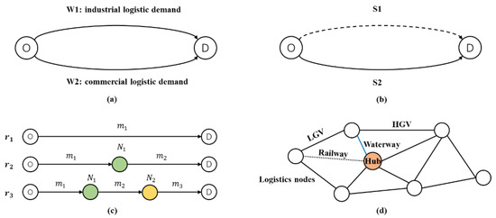
Figure 1.
Network representation of an urban logistics system. (a) Logistics user demand network . (b) Logistics service network . (c) Logistics service routes. (d) Logistics infrastructure network .
As shown in Figure 1d, a logistics infrastructure network . comprises the logistics nodes set as well as the logistics links set . More specifically, consists of a number of logistics parks, distribution centers and freight terminals, and denotes the physical links between a pair of logistics nodes which includes road segments, rail tracks, and river segments. All logistics transferring actives are conducted at logistics transfer nodes. Moreover, two groups of logistics nodes, namely logistics parks with economies of scale effects and distribution centers with smaller capacity, are considered.
To describe of the model, a virtual arc is introduced, which denotes a logistics transferring operation (e.g., the changes of transport modes). As shown in Figure 2, a logistics service along pair OD is conducted by combined transportation, which embeds a transfer from a waterway to a railway at transfer node H. To simplify the presentation, we denote as the set of logistics transfer nodes and as the set of virtual logistics transfer arcs.
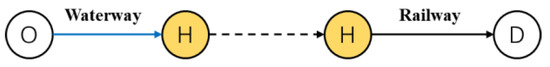
Figure 2.
Representation of a virtual transfer arc.
3.2. Assumptions
In this study, the following five basic assumptions are underlined in the city logistics network design model.
A1: The city logistics network design model is proposed to support strategic planning and policy evaluation.
A2: In the city logistics system, the logistics authority will decide the joint optimal scheme on the logistics nodes investment and CO2 emission taxes.
A3: Logistics demand originated from industrial and commercial activities are involved. The customers’ points of industry logistics demand come from the peripheral of the city, while those of commercial logistics demand arises from the city center.
A4: Logistics users tend to make their decisions for logistics service routes based on the logistics service disutility which can be evaluated by the service time and monetary cost. The monetary cost refers to the logistics cost and the CO2 emission cost [35].
A5: The introduction of road-user charging can favor a switch to other greener transport modes, such as railway and waterway. Thus, the CO2 emissions tax charges are imposed on the transport modes with high unit emissions [29].
4. Model Formulation
In the city logistics system, the logistics authority as well as logistics users (i.e., carriers) are the two interrelated decision makers. The logistics authority has to decide the optimal logistics infrastructure investments and CO2 emission taxes charges, so as to realize their objectives as much as possible. Three types of logistics infrastructure investment options are considered in this study. The first two options are to add new physical links or improve existing physical links in current logistics network, and the third one is to locate several logistics terminals in the network. The main objectives specified by the logistics authority are shown as below.
(1) Cost-recovery goal: The total logistics investment cost on the capacity enhancements of logistics infrastructures is covered by the total CO2 emissions taxes charges in the city logistics network partially or completely.
(2) Service-level goal: The total generalized logistics cost of the city logistics system is affected by the freight flow of the logistics network as well as the decisions made by the logistics authority. After introducing the logistics infrastructure investment and CO2 emissions taxes charges, a decline of the total generalized logistics cost is expected to exceed a pre-specified level.
(3) Environmental goal: The logistics authority requires that the CO2 emission decreases by a pre-specified level after the CO2 emission taxes charging and logistics capacity investment schemes are implemented.
Since above three objectives conflict with each other, favoring one of them usually weakens others. The GP approach is an effective method for us to obtain a good compromise solution among these three conflicting objectives. The goal constraints for corresponding objectives are introduced in Section 4.1.
In addition, the decisions of logistics users and the logistics authority are mutually affected by each other. From the perspective of logistics users, their decisions, which are evaluated by the perceptions of logistics service disutility, are influenced by the decisions made by the logistics authority. Conversely, the logistics authority’s decisions are affected by the routes and transport mode choices made by logistics users. These interactions can be described as a bi-level model, which can be summarized in Figure 3. We provide more detailed descriptions about the goal programming decision model based on bi-level programming in following sections.
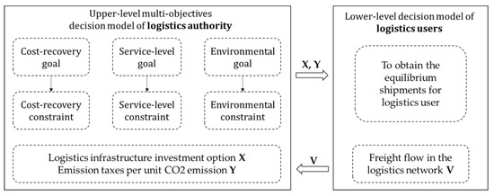
Figure 3.
Bi-level model building.
4.1. Specification of the Goal Constraints
- Cost-recovery constraint
The cost-recovery constraint implies that the total CO2 emissions taxes charges covers a pre-specified percentage of the total investment cost on expanding the capacities of the logistics infrastructures, which is defined as,
The left-hand of inequality (1) is the investment cost, while the right-hand represents the total CO2 emissions taxes charges. Parameter ϕ denotes the percentage of the total investment cost which is covered by the total CO2 emissions charges. If ϕ is smaller than 1.0, inequality (1) is a partial cost-recovery constraint. If ϕ equals 1.0, the total investment cost becomes fully covered by CO2 emissions charges. The residual part of the investment cost, that is, , is subsidized by other revenue.
The level of capacity improvement and the CO2 emissions charges determine that whether inequality (1) is satisfied. The logistics authority hopes that inequality (1) will be satisfied as closely as possible. In order to balance the left- and right-hand of inequality (1), two variables are defined to denote positive and negative deviations. Subsequently, we can obtain the equivalent constrain as Equation (2):
where the overachievement and the underachievement of the cost-recovery goal are represented by and , respectively.
- Service-level constraint
The service-level constraint states that the changes of total generalized logistics cost of city logistics system, before and after introducing the joint schemes on logistics infrastructure investment and CO2 emissions taxes charges, should reach an expected level, which is shown as follows.
The generalized logistics cost can be calculated according to the lower-level decision model of logistics users in Equations (11)–(14). Equation (3) requires that the total generalized logistics cost after carrying out joint optimization schemes of investment and CO2 emissions taxes is at most times before the joint schemes.
By introducing positive and negative deviational variables and of total generalized logistics cost regarding the corresponding target value, the goal constraint on the improvement of service level of city logistics system can be expressed as:
- Environmental constraint
The environmental constraint states that the unit of CO2 emission of the city logistics network before and after the joint schemes of logistics infrastructures investment and CO2 emission taxes charges is no more than a predefined threshold, namely, the total amount of the CO2 emissions after the joint scheme never exceeds a desired level without the joint scheme. This can be expressed as:
By introducing positive and negative deviational variables and of the CO2 emissions per unit shipment for the associated target value, the constraint (5) can be represented as Equation (8):
The parameter is a positive constant that specifies the decrease threshold of the CO2 emission of unit shipment.
4.2. Specification of the Lower-Level Decision Model of Logistics Users
As aforementioned, the logistics users’ disutility is estimated by the logistics service time, transportation cost and CO2 emission taxes, which can be defined as Equation (9):
Considering the different transportation modes, the logistics service time on link a for different modes is measured in Equation (10). A US Bureau of Public Roads-type function is applied to compute service time for HGVs and LGVs [33,49,50], while the estimation of service time spent by railways and waterways consider both the transport service time and the shift interval.
Note that is the free-flow transport service time, and is the average shift interval for transport mode m.
For each given logistics infrastructure investment options and CO2 emission charges (namely given the vector , the following model is solved to obtain the equilibrium shipments for logistics users in city logistics network [51]:
4.3. Specification of the Upper-Level Multi-Objectives Decision Model of Logistics Authority
The objective function of the GP model consists of undesired absolute deviations from the specified goal levels, where both underachievement and overachievement values are considered. The GP model is aimed to minimize these deviations under a predefined priority structures of the different goals [49].
In this paper, the priority factors of the three goals follow a decreasing order, namely, the ith goal takes precedence over the (i + 1)th goal, which is represented as follows:
where Pi is the ith priority factor, and the operator of “” represents the relative importance among various objectives of logistics authority based on the priority of decision structure. Hence, the upper-level multi-objectives decision problem can be formulated as follows:
and is subject to:
where the arc flow vectors are obtained by solving the lower-level decision model of logistics users, which is the above UE model shown as in Equations (11)–(14).
The objective function Equation (16) aims to minimize the total positive deviations from the three goals, which states that the overachievement of each goal constraint should be as low as possible. Equations (17)–(19) are the goal constraints previously defined. Equation (20) means that the CO2 emissions tax charge is non-negative and does not exceed the upper bound of charges. Equation (21) implies that logistics investment option is a 0–1 variable. Equation (22) demonstrates that at least one variable of a pair of positive and negative deviational variables is zero. Equation (23) means that the deviational variables are non-negative.
5. Solving Algorithm
This section provides an analysis on the corresponding algorithm, which solves the above proposed bi-level decision model based on goal programming. A hybrid genetic algorithm (HGA) embedded with the method of successive average (MSA) is given based on the characteristic of proposed model [50,52,53,54,55,56].
Step 1. Initialization.
(1) Initialize the important parameters of GA, which consist of the population size (pop_size), the probability of crossover (Pc) and the probability of mutation (Pm).
(2) The stopping criterion of the hybrid algorithm is defined as a certain number of generations (Max_gen) is reached.
(3) Initialize the iteration number n as zero and generate the initial population Popn = . Let the individual be the k-th decision scheme in the n-th generation; that is, is the decision vector where denote the chosen investment options and CO2 emissions tax charges, respectively.
Step 2. Calculate arc flow vectors.
Given a joint scheme , the flow of arc a by transport mode m can be obtained by solving the lower-level UE problem in Equations (9)–(14) based on the method of successive average (MSA).
Step 3. Calculate objective function.
Calculate the value of the objective function of upper-level decision model on the basis of Equations (16)–(23).
Step 4. Calculate fitness value.
The fitness value of each of Popn is calculated based on the objective function value .
Step 5. Sorting.
Sort the value fitness of individual by descending order among population .
Step 6. GA Operations.
Three operators including selection, crossover and mutation based on the value of are conducted to generate a new population . Afterwards, n is increased by 1.
Step 7. Termination check.
Check the termination condition. If the iteration number reaches max_gen, then the algorithm terminates and outputs the final solution . Otherwise, go to step 2.
5.1. Key Operators Design of Genetic Algorithm
Since the design of GA operators and the settings of parameters have a great impact on the performance of the algorithm, key elements including the coding method, selection method and crossover and mutation methods are elaborated as follows.
5.1.1. Coding Method
As shown in Figure 4, there exists two parts in the chromosome of the individual.
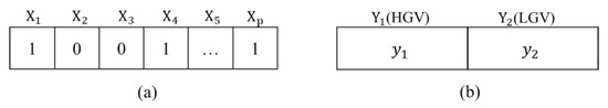
Figure 4.
Chromosome of the GA. (a) Part 1: Selection of investment projects. (b) Part 2: Unit CO2 emission taxes charges.
Part 1 means the selection of the candidate investment projects on infrastructures, in which the value of 1 represents the corresponding logistics infrastructure will be invested, otherwise, the value is 0. The values of y1 and y2 means the unit CO2 emissions taxes charges for HGV and LGV, respectively.
5.1.2. Selection Method
In this study, we employed the method of roulette wheel during the selection process. The rank-based evaluation function is also adopted.
It should be pointed out that populations are sorted in the descending order based on their fitness, i.e., the first individual (i.e., i = 1) has the best fitness, whereas the last (i.e., ) has the worst one. Additionally, the sum of the value of all individuals is equal to 1, i.e., .
The selection is conducted based on spinning the roulette wheel, which runs pop_size times. Chromosomes are selected to generate a new population in four steps as below.
Step 1. The cumulative probability for each chromosome is computed based on the following rules:
If i = 0, then , otherwise, .
Step 2. Choose a random real number .
Step 3. The i-th chromosome that satisfies is selected.
Step 4. Steps 2 and 3 are iteratively applied pop_size times to obtain chromosomes as parents for next generation.
5.1.3. Crossover and Mutation Operators
(1) Crossover operator
After selecting the operator, a new generation will be obtained by crossover and mutation operations. Considering the features of the chromosome in this study, we applied two different crossover methods. As shown in Figure 5, the two-point crossover operator is implemented for Part 1, while a convex combination method is applied for Part 2. For a given pair of parents Y1 and Y2, we can obtain two children C1 and C2 by the crossover operator as A representation crossover operation is shown in Figure 5.
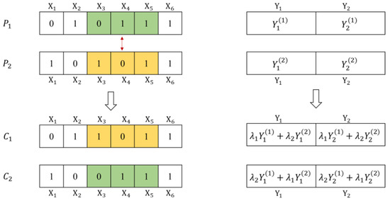
Figure 5.
Representation of the crossover operation.
(2) Mutation operator
Let r be a random positive real number no more than 1. If r < Pm, a mutation is implemented. Given a parent, is chosen for mutation. Figure 6a depicts the two-point mutation operation for vector X where the genes from position 1 to position 2 in the chromosome are reversed. With regard to the second part (i.e., vector Y), we try to update as . If is infeasible, then we replace as , which is randomly selected within the interval [0, ] until the new individual is feasible. If the above operations fail to achieve a feasible solution over certain number of iterations, is set as zero. Consequently, the new child is as shown in Figure 6b.
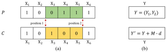
Figure 6.
Representation of the mutation operation. (a) The mutation operation for vector X. (b) The mutation operation for vector Y.
6. Case Study
6.1. Data Input
In this section, a real-world case based on the logistics network design of Changsha City, China is employed to evaluate the proposed model and solution algorithm. There are 129 links, 70 nodes as well as 32 OD pairs of logistics demand in the city logistics network. The corresponding data of the logistics network is provided in Appendix A.
Two types of logistics demand originated from industry and commercial operations are included in this logistics network. Since the logistics demands of the corresponding 32 OD pairs are unavailable, we generate this missing information by an aggregation method according to the data related to the major indicators of the National Economy and Social Development published by the Changsha Statistical Bureau. The logistics demand between each of the 32 OD pairs is provided in Table 2.
Table 2.
Logistics demand OD pairs (10,000 tons/week).
Two types of strategic decisions are adopted in investment schemes to achieve the carbon reduction goals. The first strategy is related to the subsidy on transport modes with low carbon emission (e.g., waterways and railways), while the second one is to upgrade logistic infrastructure by increasing capacities on links and logistics nodes. Forty infrastructure investment alternatives used in our case study are given in Table 3.
Table 3.
Candidate logistics infrastructure investment schemes.
The VOT is USD $10 per hour [57,58]. The transfer cost and time at the logistics transfer nodes are set according to [3,59]. The average unit emissions of HGVs, LGVs, railways and waterways are 0.132, 0.283, 0.022 and 0.016 (kg/ton-km), respectively [3,60]. The parameters of the GA are given as below. The crossover rate (Pc) and the mutation rate (Pm) are set to 0.5 and 0.1, respectively. The maximal number of generations (i.e., stopping criterion) is set to 150. These input data are considered as the base case in the following analysis unless otherwise specified.
6.2. Numerical Results and Discussion
The proposed solution algorithm was coded in C++ and run on a laptop Dell N5040 with an Intel Pentium 2.13-GHz CPU and 4.00 GB random-access memory (RAM). The CPU time for searching the corresponding optimal solution of logistics infrastructure investment options and CO2 emissions under the three different priority structures, i.e., Scenario 1: p1 = 10,000, p2 = 100, p3 = 1; Scenario 2: p1 = 100, p2 = 10,000, p3 = 1; and Scenario 3: p1 = 1, p2 = 100, p3 = 10,000.
6.2.1. Convergence of the Hybrid Genetic Algorithm Based on Frank–Wolf
The evolution progress of the proposed algorithm is depicted as Figure 7. The proposed algorithm converges after 150 generations. The average CPU searching time for each scenario is about 1015 s. Following observations are made from Figure 7 where the convergence processes of the GA under those three scenarios are depicted. First, a dramatic decline of the logarithmic values of the objective function under three different scenarios within about 40 iterations is shown in Figure 7. After 50 iterations, the logarithmic values of under all scenarios become stable. In addition, the logarithmic value of with the highest setting of priority factor p2 converges faster than other scenarios. Furthermore, the logarithmic values of with three different priority structures can converge to different levels. Overall, these results reveal that the settings of priority factor Pi have a large impact on the converged objective value while its influence of solution time can be neglected.
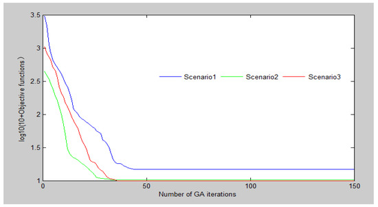
Figure 7.
Convergences of the GA algorithm under different scenarios.
6.2.2. Effects of Solution Structure of Goals on Model
In this section, we will further assess the impacts of the priority structures of goals on optimal decisions of green city network design. The following three scenarios are discussed in this study. Scenario 1 (T1): Cost-recovery goal >> Service-level goal >> Environmental goal; Scenario 2 (T2) Service-level goal >> Environmental goal >> Cost-recovery goal; and Scenario 3 (T3) Environmental goal >> Service-level goal >> Cost-recovery goal (scenarios are shown in Table 4). The cost-recovery and service-level goal are considered as the primary goal in Scenarios T1 and T2 respectively, while Scenario 3 considers the environmental goal as the primary goal.
Table 4.
Optimal CO2 emissions taxes and logistics infrastructure investment schemes under different priority structures.
From Table 4, we can see that the solutions with these three different priorities structures differ each other considerably. This observation suggests that the optimal solution is largely dependent on the priority structures of goals. Given the candidate logistics infrastructure investment options and the thresholds of the cost-recovery goal, service-level goal and environmental goal, it can be seen that the investment projects numbers and total equivalent uniform per week cost are different. That is, 11 projects with 14,880 USD/week under T1, 12 projects with 16,500 USD/week under T2 and 13 projects with 17,700 USD/week under T3. The corresponding unit shipment CO2 reduction rates are 26.6%, 35.5% and 40.7% under T1, T2 and T3, respectively. The unit CO2 emissions tax charges for HGV and LGV under T3 are 0.275 and 0.252, more than that of T2 (0.261 and 0.239) and T1 (0.272 and 0.241). This means that a higher priority rank in an environmental goal would result in much more improvement in unit shipment CO2 emissions, which also requires higher more investment costs and higher CO2 emissions tax charges.
6.2.3. Effects of Levels Structure of Goals on Achievement
A comparison on the deviational variables of scenarios T1, T2 and T3 to analyse the influence of ranking structures of the goals on the achievement levels is shown in Table 5. In Table 5, a zero value of a deviational variable implies that the associated goal is fully achieved, whereas a positive value indicates the overachievement level of the corresponding goal. Furthermore, it is obvious that all second priority goals are achieved exactly for all three different scenarios. Moreover, the environmental goal has a deviation of 8.4% from its goal level under scenario T1. When the service-level goal is regarded as the primary (i.e., T2) and the service-level goal and environmental goal can be exactly achieved, while the overachievement level of the cost-recovery goal is 17.3% of its target value. In regard to the priority structure in scenario T3, the last two goals are both completely achieved, while the overachievement level of the cost-recovery goal is 22.7% from its target value. The above observations implies that goal priority structures have a large impact on the achievements level of each goal.
Table 5.
Values of deviational variables under different priority structures.
7. Conclusions and Future Research
In this paper, an optimization model based on GP approach is proposed to address the joint optimization on logistics infrastructure investment and CO2 emissions taxes setting problem in the city logistics network, in which three decision objectives (i.e., cost-recovery objective, service-level objective and environmental one) are considered. We formulate this multi-objective optimization problem as a bi-level GP model. The upper level of the model is a GP formulation, whereas the lower level denotes a logistics service route choice user equilibrium problem. To solve the bi-level GP model, a hybrid genetic algorithm embedded with the method of successive average (MSA) is designed. The optimization model is empirically verified by a practical case study of the sustainable city logistics network in Changsha City, Hunan Province, China.
The computational experiments demonstrate the effectiveness and efficiency of the genetic algorithm for solving the bi-level GP model. The logarithmic values of the objective function under all scenarios can converge within 50 iterations. In addition, results of the case study show that the priority structures of the goals have a significant impact on decisions, as well as the achievement level of each specified goal. Higher priority ranking of the environmental goal or service-level goal can lead to a larger improvement at logistics system performance in terms of total generalized cost and unit shipment CO2 emissions. Meanwhile, the corresponding schemes also require more investment and higher CO2 emissions taxes charges. The achievement level of each goal will be conducive to improve the decision-making process by adjusting the priority structures for different goals. The proposed model and algorithm in this study provides a powerful decision support for designing a sustainable city logistics network.
Some potential directions for further research are as follows. First, some other case studies from real-world logistics networks can further verify the results of this paper and the performance of the proposed model. Second, various random factors exist in real-life cases, such as the logistics demand fluctuation, which plays a key role in the design of logistics network and management policies making. Consequently, it is essential to develop a stochastic model or robust model to cope with uncertainties in the city logistics system.
Author Contributions
Conceptualization, S.L. and D.Z.; methodology, D.Z., S.L. and Y.L.; investigation, S.L., D.Z. and Z.W.; writing—original draft preparation, S.L. and Y.L.; writing—review and editing, Y.L., Z.W. and D.Z.; supervision, D.Z., S.L. and Y.L.; funding acquisition, D.Z. and S.L. All authors have read and agreed to the published version of the manuscript.
Funding
This research was funded by the National Natural Science Foundation of China (Grant No. 71672193), Hunan Provincial Social Science Fund Project (Grant No. 19YBA378), Smart Logistics Technology Hunan Provincial Key Laboratory Project (Grant No. 2019TP1015).
Conflicts of Interest
The authors declare no conflict of interest.
Nomenclature
| Sets | |
| M | set of all transport modes, including the heavy goods vehicles (HGVs), light goods vehicles (LGVs), railways and waterways represented by “1”, “2”, “3” and “4”, respectively |
| W | set of origin–destination (OD) pairs in the logistics network |
| set of logistics service routes between OD pair | |
| K | set of logistics infrastructure investment options. “K = 1” represents improving capacities of existing infrastructures and “K = 2” represents adding new infrastructures |
| A | set of arcs, |
| A0 | set of existing arcs without logistics infrastructure investment |
| A1 | set of arcs after logistics infrastructure investment |
| General Variables | |
| the logistics demand between OD pair (tons/week) | |
| transport time over arc by transport mode m (hour) | |
| disutility on arc by transport mode m | |
| indicator variable which implies whether link a is on route r by transport mode m | |
| freight flow on route between OD pair by transport mode m (tons/week) | |
| freight flow on logistics service arc by transport mode m (tons/week) | |
| Decision Variables | |
| binary variable which equals to 1 if the logistics infrastructure investment option k over arc a is chosen and to 0 otherwise | |
| vector of binary variable , | |
| emission taxes per unit CO2 emission of transport mode m over link a ($/kg) | |
| vector of variable , | |
| Constants | |
| potential demand between OD pair by transport mode m (tons/week) | |
| free freight flow transport service time on arc by transport mode m (hour) | |
| average shift interval of transport mode m (hour) | |
| length of arc by transport mode m (km) | |
| unit transport cost on arc served by mode m ($/ton-km) | |
| the maximum capacity on arc by mode m (tons/km) | |
| the fixed cost of potential logistics infrastructures project k over link a ($/ton) | |
| value of time (VOT) ($/ton-hour) | |
| the maximum of unit CO2 emissions taxes charge ($/kg) | |
| unit CO2 emission of transport mode (kg/ton-km) | |
Appendix A
Table A1.
Basic input data for logistics networks of Changsha City, China.
Table A1.
Basic input data for logistics networks of Changsha City, China.
| Arc | From | To | Mode | Length | Time | Unit Cost | Capacity (10,000 Tons/Week) |
|---|---|---|---|---|---|---|---|
| (Km) | (Hour) | ($/Ton-Km) | |||||
| 1 | 55 | 1 | 2 | 250.00 | 3.57 | 100 | 60 |
| 2 | 1 | 7 | 2 | 2.00 | 0.03 | 0.80 | 60 |
| 3 | 7 | 11 | 2 | 2.00 | 0.03 | 0.80 | 60 |
| 4 | 11 | 18 | 2 | 9.30 | 0.13 | 3.72 | 60 |
| 5 | 18 | 23 | 2 | 6.67 | 0.10 | 2.67 | 60 |
| 6 | 23 | 53 | 2 | 260.00 | 3.71 | 104.00 | 60 |
| 7 | 52 | 1 | 2 | 156.00 | 2.23 | 62.40 | 60 |
| 8 | 52 | 11 | 2 | 152.00 | 2.17 | 60.80 | 40 |
| 9 | 52 | 29 | 2 | 150.00 | 2.14 | 60.00 | 40 |
| 10 | 52 | 18 | 2 | 155.00 | 2.21 | 62.00 | 40 |
| 11 | 52 | 23 | 2 | 162.00 | 2.31 | 64.80 | 40 |
| 12 | 11 | 12 | 2 | 4.00 | 0.06 | 1.60 | 40 |
| 13 | 55 | 43 | 3 | 250.00 | 4.17 | 75.00 | 80 |
| 14 | 18 | 19 | 2 | 5.00 | 0.07 | 2.00 | 40 |
| 15 | 23 | 24 | 2 | 2.00 | 0.03 | 0.80 | 40 |
| 16 | 1 | 2 | 2 | 8.00 | 0.11 | 3.20 | 40 |
| 17 | 7 | 8 | 2 | 11.67 | 0.17 | 4.67 | 40 |
| 18 | 12 | 13 | 2 | 4.00 | 0.06 | 1.60 | 40 |
| 19 | 12 | 29 | 2 | 3.00 | 0.04 | 1.20 | 40 |
| 20 | 29 | 19 | 2 | 7.00 | 0.10 | 2.80 | 40 |
| 21 | 19 | 20 | 2 | 7.00 | 0.10 | 2.80 | 40 |
| 22 | 24 | 25 | 2 | 6.00 | 0.09 | 2.40 | 40 |
| 23 | 55 | 3 | 2 | 250.00 | 3.57 | 100.00 | 40 |
| 24 | 2 | 3 | 2 | 3.00 | 0.04 | 1.20 | 60 |
| 25 | 2 | 13 | 2 | 6.00 | 0.09 | 2.40 | 60 |
| 26 | 24 | 53 | 2 | 260.00 | 3.71 | 104.00 | 60 |
| 27 | 13 | 14 | 2 | 3.00 | 0.04 | 1.20 | 40 |
| 28 | 42 | 66 | 1 | 8.00 | 0.20 | 3.36 | 60 |
| 29 | 3 | 8 | 2 | 4.00 | 0.06 | 1.60 | 60 |
| 30 | 8 | 14 | 2 | 4.00 | 0.06 | 1.60 | 30 |
| 31 | 14 | 20 | 2 | 11.00 | 0.16 | 4.40 | 30 |
| 32 | 20 | 25 | 2 | 4.00 | 0.06 | 1.60 | 60 |
| 33 | 3 | 4 | 2 | 12.67 | 0.18 | 5.07 | 60 |
| 34 | 8 | 9 | 2 | 9.00 | 0.13 | 3.60 | 30 |
| 35 | 14 | 15 | 2 | 20.00 | 0.29 | 8.00 | 60 |
| 36 | 20 | 21 | 2 | 8.67 | 0.12 | 3.47 | 40 |
| 37 | 32 | 33 | 2 | 2.00 | 0.03 | 0.80 | 30 |
| 38 | 64 | 34 | 2 | 5.33 | 0.08 | 2.13 | 40 |
| 39 | 25 | 34 | 2 | 9.33 | 0.13 | 3.73 | 40 |
| 40 | 34 | 48 | 2 | 10.00 | 0.14 | 4.00 | 40 |
| 41 | 34 | 49 | 2 | 8.33 | 0.12 | 3.33 | 40 |
| 42 | 45 | 43 | 0 | 1.00 | 0.50 | 5.00 | 200 |
| 43 | 43 | 50 | 3 | 40.00 | 0.67 | 12.00 | 80 |
| 44 | 55 | 4 | 2 | 250.00 | 3.13 | 100.00 | 40 |
| 45 | 4 | 9 | 2 | 4.00 | 0.06 | 1.60 | 40 |
| 46 | 4 | 5 | 2 | 11.67 | 0.17 | 4.67 | 40 |
| 47 | 9 | 31 | 2 | 11.00 | 0.16 | 4.40 | 40 |
| 48 | 21 | 32 | 2 | 10.67 | 0.15 | 4.27 | 40 |
| 49 | 31 | 16 | 2 | 6.00 | 0.09 | 2.40 | 30 |
| 50 | 31 | 43 | 3 | 8.00 | 0.20 | 3.36 | 40 |
| 51 | 15 | 60 | 1 | 5.00 | 0.13 | 2.10 | 40 |
| 52 | 16 | 33 | 2 | 9.33 | 0.13 | 3.73 | 30 |
| 53 | 15 | 33 | 1 | 8.00 | 0.20 | 3.36 | 60 |
| 54 | 34 | 26 | 2 | 7.00 | 0.10 | 2.80 | 30 |
| 55 | 33 | 27 | 2 | 11.00 | 0.16 | 4.40 | 30 |
| 56 | 26 | 27 | 2 | 4.00 | 0.06 | 1.60 | 30 |
| 57 | 27 | 53 | 2 | 260.00 | 3.71 | 104.00 | 30 |
| 58 | 5 | 31 | 2 | 3.00 | 0.04 | 1.20 | 30 |
| 59 | 51 | 5 | 2 | 6.00 | 0.09 | 2.40 | 30 |
| 60 | 55 | 44 | 4 | 280.00 | 7.00 | 70.00 | 80 |
| 61 | 44 | 48 | 4 | 41.00 | 1.03 | 10.25 | 120 |
| 62 | 55 | 6 | 2 | 270.00 | 3.38 | 108.00 | 30 |
| 63 | 5 | 6 | 2 | 8.00 | 0.11 | 3.20 | 30 |
| 64 | 6 | 54 | 2 | 163.00 | 2.33 | 65.20 | 30 |
| 65 | 46 | 18 | 0 | 2.00 | 0.50 | 10.00 | 100 |
| 66 | 31 | 10 | 3 | 11.00 | 0.18 | 3.30 | 40 |
| 67 | 10 | 54 | 3 | 160.00 | 2.67 | 48.00 | 40 |
| 68 | 10 | 47 | 3 | 32.00 | 0.53 | 9.60 | 30 |
| 69 | 6 | 17 | 2 | 6.00 | 0.09 | 2.40 | 60 |
| 70 | 16 | 17 | 2 | 8.00 | 0.11 | 3.20 | 30 |
| 71 | 17 | 54 | 2 | 155.00 | 2.21 | 62.00 | 30 |
| 72 | 17 | 22 | 2 | 13.00 | 0.19 | 5.20 | 30 |
| 73 | 33 | 22 | 2 | 11.00 | 0.16 | 4.40 | 30 |
| 74 | 22 | 54 | 2 | 165.00 | 2.36 | 66.00 | 30 |
| 75 | 22 | 28 | 2 | 7.00 | 0.10 | 2.80 | 80 |
| 76 | 27 | 28 | 2 | 9.00 | 0.13 | 3.60 | 40 |
| 77 | 28 | 54 | 2 | 155.00 | 2.21 | 62.00 | 40 |
| 78 | 28 | 53 | 2 | 260.00 | 3.71 | 104.00 | 40 |
| 79 | 46 | 29 | 0 | 3.00 | 0.50 | 15.00 | 100 |
| 80 | 56 | 39 | 1 | 4.00 | 0.10 | 1.68 | 80 |
| 81 | 57 | 39 | 1 | 5.00 | 0.13 | 2.10 | 100 |
| 82 | 39 | 66 | 1 | 6.00 | 0.15 | 2.52 | 80 |
| 83 | 66 | 35 | 1 | 4.00 | 0.10 | 1.68 | 40 |
| 84 | 66 | 37 | 1 | 9.00 | 0.23 | 3.78 | 40 |
| 85 | 65 | 35 | 1 | 9.00 | 0.23 | 3.78 | 40 |
| 86 | 65 | 37 | 1 | 4.00 | 0.10 | 1.68 | 40 |
| 87 | 37 | 64 | 1 | 6.00 | 0.15 | 2.52 | 40 |
| 88 | 65 | 41 | 1 | 5.00 | 0.13 | 2.10 | 40 |
| 89 | 41 | 64 | 1 | 5.00 | 0.13 | 2.10 | 40 |
| 90 | 70 | 41 | 1 | 5.00 | 0.13 | 2.10 | 40 |
| 91 | 41 | 69 | 1 | 4.00 | 0.10 | 1.68 | 60 |
| 92 | 49 | 48 | 0 | 2.00 | 0.50 | 10.00 | 100 |
| 93 | 45 | 44 | 0 | 2.00 | 0.50 | 10.00 | 150 |
| 94 | 45 | 4 | 0 | 2.00 | 0.50 | 10.00 | 150 |
| 95 | 40 | 59 | 1 | 4.00 | 0.10 | 1.68 | 80 |
| 96 | 40 | 15 | 1 | 4.00 | 0.10 | 1.68 | 80 |
| 97 | 36 | 15 | 1 | 2.00 | 0.05 | 0.84 | 60 |
| 98 | 36 | 61 | 1 | 8.00 | 0.20 | 3.36 | 60 |
| 99 | 38 | 61 | 1 | 10.00 | 0.25 | 4.20 | 60 |
| 100 | 64 | 38 | 1 | 2.00 | 0.05 | 0.84 | 60 |
| 101 | 42 | 65 | 1 | 5.00 | 0.13 | 2.10 | 80 |
| 102 | 42 | 67 | 1 | 5.00 | 0.13 | 2.10 | 60 |
| 103 | 42 | 68 | 1 | 3.00 | 0.08 | 1.26 | 60 |
| 104 | 46 | 19 | 0 | 1.00 | 0.50 | 5.00 | 40 |
| 105 | 19 | 24 | 2 | 7.00 | 0.10 | 2.80 | 30 |
| 106 | 51 | 55 | 2 | 266.00 | 3.80 | 106.40 | 30 |
| 107 | 32 | 26 | 2 | 9.00 | 0.13 | 3.60 | 30 |
| 108 | 62 | 47 | 1 | 5.00 | 0.13 | 2.10 | 40 |
| 109 | 49 | 50 | 0 | 3.00 | 0.50 | 15.00 | 80 |
| 110 | 47 | 53 | 3 | 260.00 | 4.33 | 78.00 | 30 |
| 111 | 48 | 53 | 4 | 250.00 | 6.25 | 62.50 | 120 |
| 112 | 49 | 53 | 2 | 250.00 | 3.57 | 100.00 | 30 |
| 113 | 50 | 53 | 3 | 250.00 | 4.17 | 75.00 | 80 |
| 114 | 63 | 48 | 1 | 4.00 | 0.50 | 20.00 | 60 |
| 115 | 8 | 56 | 0 | 0.50 | 0.50 | 2.50 | 80 |
| 116 | 9 | 57 | 0 | 0.50 | 0.50 | 2.50 | 80 |
| 117 | 31 | 58 | 0 | 0.50 | 0.50 | 2.50 | 60 |
| 118 | 31 | 59 | 0 | 0.50 | 0.50 | 2.50 | 60 |
| 119 | 16 | 60 | 0 | 0.50 | 0.50 | 2.50 | 60 |
| 120 | 32 | 61 | 0 | 0.50 | 0.50 | 2.50 | 40 |
| 121 | 27 | 62 | 0 | 0.50 | 0.50 | 2.50 | 60 |
| 122 | 27 | 63 | 0 | 0.50 | 0.50 | 2.50 | 150 |
| 123 | 21 | 64 | 0 | 0.50 | 0.50 | 2.50 | 200 |
| 124 | 20 | 65 | 0 | 0.50 | 0.50 | 2.50 | 100 |
| 125 | 14 | 66 | 0 | 0.50 | 0.50 | 2.50 | 60 |
| 126 | 29 | 67 | 0 | 0.50 | 0.50 | 2.50 | 60 |
| 127 | 19 | 68 | 0 | 0.50 | 0.50 | 2.50 | 60 |
| 128 | 34 | 69 | 0 | 0.50 | 0.50 | 2.50 | 100 |
| 129 | 25 | 70 | 0 | 0.50 | 0.50 | 2.50 | 100 |
Note: In “mode” column, HGV, LGV, Railway and Waterway are indexed by 1, 2, 3 and 4 respectively, and the virtual logistics transfer arc in logistics nodes is indexed by 0. (Source: Data adapted from reference [28,51]).
References
- Firdausiyah, N.; Taniguchi, E.; Qureshi, A. Modeling city logistics using adaptive dynamic programming based multi-agent simulation. Transp. Res. Part E Logist. Transp. Rev. 2019, 125, 74–96. [Google Scholar] [CrossRef]
- Thompson, R.G.; Zhang, L. Optimising courier routes in central city areas. Transp. Res. Part C Emerg. Technol. 2018, 93, 1–12. [Google Scholar] [CrossRef]
- Qu, Y.; Bektaş, T.; Bennell, J. Sustainability SI: Multimode Multicommodity Network Design Model for Intermodal Freight Transportation with Transfer and Emission Costs. Netw. Spat. Econ. 2016, 16, 303–329. [Google Scholar] [CrossRef]
- McKinnon, A.; Halldorsson, A.; Rizet, C. Theme issue on sustainable freight transport. Res. Transp. Bus. Manag. 2014, 12, 1–2. [Google Scholar] [CrossRef]
- Russo, F.; Comi, A. Investigating the Effects of City Logistics Measures on the Economy of the City. Sustainability 2020, 12, 1439. [Google Scholar] [CrossRef]
- Gómez-Marín, C.G.; Serna-Urán, C.A.; Arango-Serna, M.D.; Comi, A. Microsimulation-Based Collaboration Model for Urban Freight Transport. IEEE Access 2020, 8, 182853–182867. [Google Scholar] [CrossRef]
- Zhang, D.Z.; Zhan, Q.W.; Chen, Y.C.; Li, S.Y. Joint optimization of logistics infrastructure investments and subsidies in a regional logistics network with CO2 emission reduction targets. Transp. Res. Part D Transp. Environ. 2018, 60, 174–190. [Google Scholar] [CrossRef]
- Dablanc, L.; Ross, C. Atlanta: A mega logistics center in the Piedmont Atlantic Megaregion (PAM). J. Transp. Geogr. 2012, 24, 432–442. [Google Scholar] [CrossRef]
- Wang, C.-X. Optimization of Hub-and-Spoke Two-stage Logistics Network in Regional Port Cluster. Syst. Eng. Theory Pract. 2008, 28, 152–158. [Google Scholar] [CrossRef]
- O’Kelly, M.E. Hub location with flow economies of scale. Transp. Res. Part B Methodol. 1998, 32, 605–616. [Google Scholar] [CrossRef]
- Lin, C.-C.; Lee, S.-C. The competition game on hub network design. Transp. Res. Part B Methodol. 2010, 44, 618–629. [Google Scholar] [CrossRef]
- Lin, C.-C.; Chen, S.-H. An integral constrained generalized hub-and-spoke network design problem. Transp. Res. Part E Logist. Transp. Rev. 2008, 44, 986–1003. [Google Scholar] [CrossRef]
- Alumur, S.A.; Kara, B.Y.; Karasan, O.E. Multimodal hub location and hub network design. Omega 2012, 40, 927–939. [Google Scholar] [CrossRef]
- Szeto, W.Y.; Jaber, X.; Wong, S.C. Road Network Equilibrium Approaches to Environmental Sustainability. Transp. Rev. 2012, 32, 491–518. [Google Scholar] [CrossRef]
- Li, Z.-C.; Ge, X.-Y. Traffic signal timing problems with environmental and equity considerations. J. Adv. Transp. 2014, 48, 1066–1086. [Google Scholar] [CrossRef]
- Melo, M.T.; Nickel, S.; Saldanha-da-Gama, F. Facility location and supply chain management—A review. Eur. J. Oper. Res. 2009, 196, 401–412. [Google Scholar] [CrossRef]
- Hurley, W.J.; Petersen, E.R. Nonlinear tariffs and freight network equilibrium. Transp. Sci. 1994, 28, 236–245. [Google Scholar] [CrossRef]
- Harker, P.T.; Friesz, T.L. Prediction of intercity freight flows, 2: Mathematical formulations. Transp. Res. Part B Methodol. 1986, 20, 155–174. [Google Scholar] [CrossRef]
- Yang, H.; Bell, M.G.H. Models and algorithms for road network design: A review and some new developments. Transp. Rev. 1998, 18, 257–278. [Google Scholar] [CrossRef]
- Friesz, T.L.; Tobin, R.L.; Harker, P.T. Predictive intercity freight network models—The state of the art. Transp. Res. Part A Policy Pract. 1983, 17, 409–417. [Google Scholar] [CrossRef]
- Li, Z.-C.; Lam, W.H.K.; Wong, S.C. Modeling intermodal equilibrium for bimodal transportation system design problems in a linear monocentric city. Transp. Res. Part B Methodol. 2012, 46, 30–49. [Google Scholar] [CrossRef]
- Guelat, J.; Florian, M.; Crainic, T.G. A multimode multiproduct network assignment model for strategic-planning of freight flows. Transp. Sci. 1990, 24, 25–39. [Google Scholar] [CrossRef]
- Yamada, T.; Russ, B.F.; Castro, J.; Taniguchi, E. Designing Multimodal Freight Transport Networks: A Heuristic Approach and Applications. Transp. Sci. 2009, 43, 129–143. [Google Scholar] [CrossRef]
- Catalano, M.; Migliore, M. A Stackelberg-game approach to support the design of logistic terminals. J. Transp. Geogr. 2014, 41, 63–73. [Google Scholar] [CrossRef]
- Crainic, T.G. Service network design in freight transportation. Eur. J. Oper. Res. 2000, 122, 272–288. [Google Scholar] [CrossRef]
- Crainic, T.G.; Ricciardi, N.; Storchi, G. Models for Evaluating and Planning City Logistics Systems. Transp. Sci. 2009, 43, 432–454. [Google Scholar] [CrossRef]
- SteadieSeifi, M.; Dellaert, N.P.; Nuijten, W.; Van Woensel, T.; Raoufi, R. Multimodal freight transportation planning: A literature review. Eur. J. Oper. Res. 2014, 233, 1–15. [Google Scholar] [CrossRef]
- Dekker, R.; Bloemhof, J.; Mallidis, I. Operations Research for green logistics—An overview of aspects, issues, contributions and challenges. Eur. J. Oper. Res. 2012, 219, 671–679. [Google Scholar] [CrossRef]
- McKinnon, A.C.; Cullinane, S.; Browne, M.; Whiteing, A. Green Logistics: Improving the Environmental Sustainability of Logistics; Kogan Page Ltd.: New York, NY, USA, 2012. [Google Scholar]
- Elhedhli, S.; Merrick, R. Green supply chain network design to reduce carbon emissions. Transp. Res. Part D Transp. Environ. 2012, 17, 370–379. [Google Scholar] [CrossRef]
- Harris, I.; Naim, M.; Palmer, A.; Potter, A.; Mumford, C. Assessing the impact of cost optimization based on infrastructure modelling on CO2 emissions. Int. J. Prod. Econ. 2011, 131, 313–321. [Google Scholar] [CrossRef]
- Rudi, A.; Fröhling, M.; Zimmer, K.; Schultmann, F. Freight transportation planning considering carbon emissions and in-transit holding costs: A capacitated multi-commodity network flow model. EURO J. Transp. Logist. 2014, 5, 123–160. [Google Scholar] [CrossRef]
- Nagurney, A.; Toyasaki, F. Supply chain supernetworks and environmental criteria. Transp. Res. Part D Transp. Environ. 2003, 8, 185–213. [Google Scholar] [CrossRef]
- Zhang, D.; Eglese, R.; Li, S. Optimal location and size of logistics parks in a regional logistics network with economies of scale and CO2 emission taxes. Transport 2015, 33, 52–68. [Google Scholar] [CrossRef]
- Yin, Y.; Li, Z.C.; Lam, W.H.K.; Choi, K. Sustainable Toll Pricing and Capacity Investment in a Congested Road Network: A Goal Programming Approach. J. Transp. Eng. 2014, 140, 04014062. [Google Scholar] [CrossRef]
- Chen, K.; Yang, Z.Z.; Notteboom, T. The design of coastal shipping services subject to carbon emission reduction targets and state subsidy levels. Transp. Res. Part E Logist. Transp. Rev. 2014, 61, 192–211. [Google Scholar] [CrossRef]
- Gao, X.; Cao, C. A novel multi-objective scenario-based optimization model for sustainable reverse logistics supply chain network redesign considering facility reconstruction. J. Clean. Prod. 2020, 270, 122405. [Google Scholar] [CrossRef]
- Wang, F.; Lai, X.; Shi, N. A multi-objective optimization for green supply chain network design. Decis. Support Syst. 2011, 51, 262–269. [Google Scholar] [CrossRef]
- Harris, I.; Mumford, C.L.; Naim, M.M. A hybrid multi-objective approach to capacitated facility location with flexible store allocation for green logistics modeling. Transp. Res. Part E Logist. Transp. Rev. 2014, 66, 1–22. [Google Scholar] [CrossRef]
- Yuchi, Q.; Wang, N.; Li, S.; Yang, Z.; Jiang, B. A bi-objective reverse logistics network design under the emission trading scheme. IEEE Access 2019, 7, 105072–105085. [Google Scholar] [CrossRef]
- Chen, C.; Hu, X.; Gan, J.; Qiu, R. Regional low-carbon timber logistics network design and management using multi-objective optimization. J. For. Res. 2017, 22, 354–362. [Google Scholar] [CrossRef]
- Jiang, J.; Zhang, D.; Meng, Q.; Liu, Y. Regional multimodal logistics network design considering demand uncertainty and CO2 emission reduction target: A system-optimization approach. J. Clean. Prod. 2020, 248, 119304. [Google Scholar] [CrossRef]
- Samuel, C.N.; Venkatadri, U.; Diallo, C.; Khatab, A. Robust closed-loop supply chain design with presorting, return quality and carbon emission considerations. J. Clean. Prod. 2020, 247, 119086. [Google Scholar] [CrossRef]
- Van Engeland, J.; Beliën, J.; De Boeck, L.; De Jaeger, S. Literature review: Strategic network optimization models in waste reverse supply chains. Omega 2020, 91, 102012. [Google Scholar] [CrossRef]
- Liu, Q.; Li, X.; Liu, H.; Guo, Z. Multi-objective metaheuristics for discrete optimization problems: A review of the state-of-the-art. Appl. Soft Comput. 2020, 93, 106382. [Google Scholar] [CrossRef]
- Charnes, A.; Cooper, W.W.; Ferguson, R.O. Optimal Estimation of Executive Compensation by Linear Programming. Manag. Sci. 1955, 1, 138–151. [Google Scholar] [CrossRef]
- Chen, A.; Xu, X. Goal programming approach to solving network design problem with multiple objectives and demand uncertainty. Expert Syst. Appl. 2012, 39, 4160–4170. [Google Scholar] [CrossRef]
- Bal, A.; Satoglu, S.I. A goal programming model for sustainable reverse logistics operations planning and an application. J. Clean. Prod. 2018, 201, 1081–1091. [Google Scholar] [CrossRef]
- Tamiz, M.; Jones, D.; Romero, C. Goal programming for decision making: An overview of the current state-of-the-art. Eur. J. Oper. Res. 1998, 111, 569–581. [Google Scholar] [CrossRef]
- Nguyen, S.; Pallottino, S.; Gendreau, M. Implicit enumeration of hyperpaths in a logit model for transit networks. Transp. Sci. 1998, 32, 54–64. [Google Scholar] [CrossRef]
- Sheffi, Y. Urban Transportation Networks: Equilibrium Analysis with Mathematical Programming Methods; Prentice-Hall: Englewood Cliffs, NJ, USA, 1985. [Google Scholar]
- Geoffrion, A.M. An improved implicit enumeration approach for integer programming. Oper. Res. 1969, 17, 437–454. [Google Scholar] [CrossRef][Green Version]
- Li, Z.-C.; Lam, W.H.; Wong, S. Optimization of number of operators and allocation of new lines in an oligopolistic transit market. Netw. Spat. Econ. 2012, 12, 1–20. [Google Scholar] [CrossRef][Green Version]
- Luathep, P.; Sumalee, A.; Lam, W.H.K.; Li, Z.-C.; Lo, H.K. Global optimization method for mixed transportation network design problem: A mixed-integer linear programming approach. Transp. Res. Part B Methodol. 2011, 45, 808–827. [Google Scholar] [CrossRef]
- Baoding, L. Dependent-chance goal programming and its genetic algorithm based approach. Math. Comput. Model. 1996, 24, 43–52. [Google Scholar] [CrossRef]
- Cheng, C.; Zhu, R.; Costa, A.M.; Thompson, R.G.; Huang, X. Multi-period two-echelon location routing problem for disaster waste clean-up. Transp. A Transp. Sci. 2021, 1–31. [Google Scholar] [CrossRef]
- De Jong, G.; Kouwenhoven, M.; Bates, J.; Koster, P.; Verhoef, E.; Tavasszy, L.; Warffemius, P. New SP-values of time and reliability for freight transport in the Netherlands. Transp. Res. Part E Logist. Transp. Rev. 2014, 64, 71–87. [Google Scholar] [CrossRef]
- Guan, H.-Z.; Kazuo, N. Study on Estimation of the Time Value in Freight Transport. J. Highw. Transp. Res. Dev. 2000, 17, 5. [Google Scholar]
- Yong, Z. Guang Zhou River Logistics Park Project Risk Management Research. Master’s Thesis, South China University of Technology, Guangzhou, China, 2011. [Google Scholar]
- Bajeux-Besnainou, I.; Joshi, S.; Vonortas, N. Uncertainty, networks and real options. J. Econ. Behav. Organ. 2010, 75, 523–541. [Google Scholar] [CrossRef]


Publisher’s Note: MDPI stays neutral with regard to jurisdictional claims in published maps and institutional affiliations. |
© 2021 by the authors. Licensee MDPI, Basel, Switzerland. This article is an open access article distributed under the terms and conditions of the Creative Commons Attribution (CC BY) license (https://creativecommons.org/licenses/by/4.0/).