Prevention Is Better Than Cure: Machine Learning Approach to Conflict Prediction in Sub-Saharan Africa

Abstract

This article offers policymakers and researchers pragmatic and sustainable approaches to identify and mitigate conflict threats by looking beyond p-values and plausible instruments. We argue that predicting conflict successfully depends on the choice of algorithms, which, if chosen accurately, can reduce economic and social instabilities caused by post-conflict reconstruction. After collating data with variables linked to conflict, we used a grid level dataset of 5928 observations spanning 48 countries across sub-Saharan Africa to predict civil conflict. The goals of the study were to assess the performance of supervised classification machine learning (ML) algorithms in comparison with logistic model, assess the implication of selecting a specific performance metric on policy initiatives, and evaluate the value of interpretability of the selected model. After comparing class imbalance resampling methods, the synthetic minority over-sampling technique (SMOTE) was employed to improve out-of-sample prediction for the trained model. The results indicate that if our selected performance metric is recall, gradient tree boosting is the best algorithm; however, if precision or F1 score is the selected metric, then the multilayer perceptron algorithm produces the best model.

1. Introduction

“For many decision problems, it may be that prediction is of primary importance, and inference is at best of secondary importance. Even in cases where it is possible to do inference, it is important to keep on mind that the requirements that ensure this ability often come at the expense of predictive performance [1].”

From a policy perspective, accurately predicting the occurrence of civil conflict can reduce economic and social costs [2]. In 2017, the global economic impact of violence was estimated at 12.4 percent of world GDP ($14.6 trillion in purchasing power parity) [3]. Over the past six decades, the per capita growth has been three times higher in highly peaceful countries than in those with low levels of peace. This implies that allocating resources to predicting and preventing violence has significant positive economic benefits. In studies that evaluate the economic cost of conflict/violence, two areas are analyzed: (i) costs that arise as a consequence of violence and (ii) the expenditures to prevent violence. While it appears that expenditures to prevent violence may be less expensive, policymakers are skeptical of implementing prevention measures as they are viewed as riskier or even futile in the presence of erroneous prediction models. However, we argue that using multiple classification algorithms to select the best predictive model can alleviate such confusion, reduce or eliminate costs due to conflict, and most importantly, save human lives. Thus, our research offers empirical explorations and comparisons of logistic and machine learning algorithms that predict conflict and thereby minimize the economic and social costs of civil conflict.

Machine learning approaches empirical analysis as algorithms that estimate and compare different alternate scenarios. This fundamentally differs from econometric analysis, where the researcher chooses a specification based on principles and estimates the best model. Instead, machine learning is based on improving and changing models dynamically, which is data-driven. It enables researchers and policymakers to improve their predictions and analysis over time with evolving technology and data points. While research on conflict and violence in economic and policy sciences has progressed substantially in recent times, most of this literature focuses on identifying the possible drivers of conflict while ensuring the underlying assumptions of the data-generating process are met [4,5]. Model selection in such an econometric analysis of conflict is dominated by issues of identification, variable direction, as well as the magnitude of estimates, thereby imposing additional constraint on the response of policymakers. Most of the contemporary literature draws a causal connection to conflict with sociopolitical and geographic variables [6,7,8,9], whereby researchers identify variables and their associated, unbiased coefficients that cause conflict. The general goal is to maximize the t-statistic, thereby increasing estimation confidence and averting a type II error. However, we ask if from a policy perspective, are these investigations effective in mitigating, and more importantly, preventing conflict? We argue that conflict prevention is better than incurring the costs of conflict. Accordingly, we reformulate the research question to whether a region is susceptible to imminent conflict through a comparison of different econometric and machine learning models.

To examine how binary choice algorithms used in traditional econometrics compares to supervised machine learning algorithms, we have carefully synthesized data on violent conflict, geographical, socioeconomic, political, and agricultural variables. We used data from the Armed Conflict Location and Event Data (ACLED) Project [10], which records violence prevalence information, as opposed to the Uppsala Conflict Data Program (UCDP) database, which codes civil war onset and fatality information [5,11]. Our rationale for this approach lies in our efforts to impact policy changes at a state or district level. Our approach of including a larger sphere of conflict events, especially less fatal ones, has the potential of generating effective policy pathways to prevent mass atrocities. Conflict prevention or mitigation goes beyond civil war deterrence and the promotion of peace. Often, smaller events are warning signs which, if detected, can prevent potential civil wars. Our combined variables are scaled to a 0.5 × 0.5-degree grid scale. The ACLED data provides information on the prevalence of conflict events including battles, violence against civilians, remote violence, rioting and protesting against a government, and non-violent conflict within the context of war. Next, we have identified and described a set of novel and standard prediction algorithms currently dominating the machine learning literature. Machine learning provides a set of algorithms that can be used to improve prediction accuracy over classic predictive techniques such as logistic algorithm. Supervised (classification) machine learning (ML) approaches have gained popularity due to their ability to outperform simple algorithms such as logistic algorithms, providing more accurate out-of-sample predictions [12]. In as much as ML-supervised algorithms have gained popularity, their use in conflict prediction is still limited and class imbalance is not explicitly addressed [13,14]. Imbalance occurs when the number of observations reporting conflict are not equally distributed, and this might bias the algorithm’s out-of-sample prediction towards the dominant class (observations or locations without conflict). In our study, we have explicitly addressed classification imbalance. We argue that policymakers can obtain good prediction on incidences of conflict using existing data and applying ML algorithms that can assist in developing the best model for identifying the onset of conflict, thus reducing socioeconomic costs. Finally, we have compared the performances of the logistic model (binary choice model) against four machine learning algorithms and subsequently discuss the best path forward for policymakers.

Contemporary studies on conflict prediction suffer from a few drawbacks, as discussed in detail in the following section. To begin with, most of these studies are limited in their geographical scope or use of high-resolution data. Furthermore, they often indicate low performance in accuracy. Finally, in cases where multiple models are compared, the studies neither explicitly illustrate how addressing imbalance increases model performance nor compare predictive performance between using a reduced set of indicators. In contrast, our initiative distinguishes and contributes to the novel yet emerging body of literature on conflict prediction in the following ways. First, in the realm of the machine learning and conflict mitigation literature, our synthesized datasets are exhaustive and fine-combed. Our study spans over 40 countries in sub-Saharan Africa and examines conflict at a finer grid resolution within each country to predict conflict incidences at a sub-national level. From a policy perspective, our model selection is data driven, whereby a large range of models are considered. However, we have carefully selected confidence intervals as well as document model selection processes. Second, while our intention is neither to carry out causal analysis nor impact evaluation, we have listed the top 25 predictors of conflict that may assist policymakers. We hope that our efforts can at least enable policymakers to focus on a few key drivers of conflict. Third, and most importantly, we have compared performances across five classification algorithms while addressing issues of class imbalance that are pervasive in conflict analysis and provide information on the best imbalance resampling methods that provides the most accurate prediction. Additionally, we compare the differences on the possible efficacy and precision of these models. While the philosophical and scientific needs to investigate the drivers of conflict are undeniable, policy prescription needs to be pragmatic. In our model comparisons, we examine the gains obtained from using different ML models in comparison to the logistic model and discuss how performance metrics of the models may be of different value to different policy markers given the context. The trade-off between the models depends on the objective that the policymaker wants to achieve. Traditional causal analysis of conflict puts emphasis on in-sample prediction power and extreme caution towards not accepting a false hypothesis. However, for successful policies to prevent random yet fatal conflict, out-of-sample predictions along with caution towards neglecting harbingers of catastrophic uprising, i.e., rejecting the true hypotheses, may be more important. ML classification prediction problems are focused on a lower classification error and thereby provide a much better approach. The performance metrics shed light on the important policy conundrum of deciding whether institutions should prioritize preventing conflict or preserving resources for post-conflict development.

The rest of this article is structured as follows: the review section presents the current literature to identify variables and causal structures; the data and variable selection sections describes the source of the data and provides context; the results, discussion, and conclusion sections present the results and discuss their importance and contributions to the current scholarship.

2. Literature Review

A third of the countries in sub-Saharan Africa have been involved in some kind of civil war (defined as more than 1000 battle deaths per annum) or conflict from the mid-1990s. An estimated 750,000 to 1.1 million people were killed in conflict in Africa between 1989 and 2010 [15]. The potential costs of conflict can include a substantial loss of lives, monetary losses, loss in investment and state capacity, forced displacement and mass migration, and an eventual breakdown of social cohesion, institutions, and norms [3,15,16,17,18,19,20,21].

Social scientists across disciplines agree that there are four main drivers of conflict: lack of socioeconomic development, low capabilities of the state, intergroup inequality, and recent history of violent conflict [7,22,23]. Socioeconomic development includes low per capita income, slow economic growth, high natural resource dependence, low levels of education, and high population [7,9,24,25,26,27,28]. Valid causal claims are usually argued for either by exploiting exogenous sources of variation such as price shocks or natural resource endowment including diamonds and petroleum [28] or the use of instruments such as rainfall and rainfall growth [7,24]. State institutional capabilities that often reflect how favorable or unfavorable conditions are to insurgents include a lack of democracy, poor governance, fragile institutions, weak militaries, and rough terrains. The seminal works of both Collier and Hoeffler [4,9] and Fearon and Laitin [27] establish that the roots of civil wars lie largely in opportunities for insurgency (through channels mentioned above, such as fragile institutions and poor governance) and are not driven by political grievances. However, this stands in contradiction to proponents who argue that intergroup inequality and political grievances arising from ethnic and religious fractionalization across groups lead to civil conflict. Drivers of violent conflict can include both spatial as well as temporal aspects, whereby a history of violent conflict in the past affects future conflict. In addition, agrarian societies, such as most of sub-Saharan Africa, are vulnerable to conflict arising from loss of agricultural income (a key livelihood activity), grievances from fluctuations in yield and productivity, and price shocks as well as weather shocks.

Most existing studies on civil war onset have poor predictive power and place more importance on causal inference and the statistical significance of individual variables. However, such statistical significance is sensitive to model specification as well as high-quality data availability [5,11,29,30]. For example, the often-cited logistic models used by Collier and Hoeffler [9] or Fearon and Laitin [27] tend to have less than 10 percent accuracy for the prediction of war onset [5]. Using a multinomial logit model along with out-of-sample validation and a threshold of p > 0.3 for positive prediction, Hegre et al.’s [11] model is much more effective at arriving at a true positive rate of 0.71, and a corresponding false positive rate of 0.085, seven to nine years into the future.

In contrast, statistical machine learning models appear to have superior performance when predicting conflict onset. For example, using data from Columbia and Indonesia, Bazzi et al. [31] show that ML models are reliably able to identify persistent high-violence hot spots. Chadefaux [32] uses logit models to predict the onset of war with high confidence in relatively shorter time spans. Muchlinski et al. [30] finds that random forest algorithms can correctly predict 9 out of 20 civil wars, compared to zero correct predictions by three conventional logistic models (classic, Firth rare events, and L1-regularized). This result is supported by Mueller and Rauh [33], who use text mining to show that a random forest model performs extremely well in predicting conflict outbreaks, especially in previously peaceful countries. However, most conflict prediction models rely on national-level aggregated statistics, which ignores within-country variation and may not be representative of local contexts. Despite advances in both geospatial analysis and more sophisticated ML algorithms, conflict prediction models have rarely combined the two (granular geospatial data with ML algorithms). Only a handful of recent studies use sub-national data to predict conflict [34,35,36]. For example, van Weezel [36] uses sub-national data on Africa to analyze the predictive performance of a model of violent armed conflict with a range of geographic and socio-economic predictors commonly used in the causal literature. The study uses data from 2000 to 2009 to make out-of-sample predictions for 2010 to 2015 and provides an overview of the predictors of local-level conflict in Africa. The author finds that conflict dynamics, determined by lagged values of spatial and temporal conflict incidences, represent the strongest predictor of future conflict. Furthermore, persistence of conflict is easier to predict than the onset of new conflict events. A similar study is presented in Perry [35] with the added advantage of using two ML algorithms—a Naïve Bayes and random forest model—to predict district-level conflict in Africa from 1997 to 2012. The study finds that selecting appropriate ML models can lead to substantial improvements in accuracy and performance and that using full models offers more predictive power than using a prior outbreak of violence as the main indicator of current violence. Overall, the study found that random forest has an accuracy of 58.5%, while Naïve Bayes produces an accuracy of 24.6%. One drawback of the study is that it uses battle events as the only indicator of political violence, though the author acknowledges that other categories of conflict events, such as riots, protests, violence against civilians, remote violence, etc., should be included for more complete models of fragility and conflict prediction. Gill [34] compares the performance of a logistic model with a random forest model in predicting political violence (defined as civil war battles and violence against civilians) in West Africa. District-level data for the period of 2015 to 2017 was used to train the model prior to making out-of-sample predictions for 2018. The study did not find a significant difference between the performance of the two models, with an accuracy of about 74.7% for the logistic model and 78.4% for random forest. The predictive power of the random forest model with an F1 score of 0.58582 is similar to Perry [35], but the logistic regression model produces an F1 score of 0.61017, which indicates better performance than the F1 score of 0.257 in Weezel [36]. The variables in the study that contribute the most to predictive power in both models include conflict density, road density, the area of the district, nighttime lights, and population density. Overall, the author found that the logistic regression model slightly outperforms the random forest model. One drawback of the study is that it is restricted to West Africa and uses district-level data. In contrast, our study uses fine-combed data from 40 countries across sub-Saharan Africa and compares between five classification algorithms to predict conflict while addressing class imbalance issues.

3. Data

To measure conflict, we use the Armed Conflict Location and Event Data Project (ACLED), version 7, developed by the International Peace Research Institute of Oslo, Norway, and the University of Uppsala, Sweden (referred to as PRIO/Uppsala); obtained from Raleigh et al. (2010). This dataset documents nine different types of civil and communal conflict events in African states, from a period of 1997 to 2016, including battles, violence against civilians, remote violence, rioting and protesting against a government, and non-violent conflict within the context of the war. Most of the contemporary literature that use Uppsala data only considers battle-related deaths that resulted in fatalities of over 10,000. However, by fine-combing and considering the aforementioned smaller-scale violence events, we expect to offer more robust models. We obtained crop data from the Spatial Production and Allocation Model (SPAM), 2005 version 1.0. This data was developed by the Food and Agricultural Organization (FAO), International Food Policy Research Institute (IFPRI), and the Center for Sustainability and the Global Environment (SAGE) at the University of Wisconsin-Madison. SPAM 2005 uses national and sub-national-level crop statistics (averaged and standardized over a period of three years from 2004 to 2006 to FAO country levels) and provides detailed grid-level information—such as crops cultivated, irrigation practices, inputs used, yield, production, etc.—for 42 crops.

We have combined large and publicly available datasets at a resolution of 0.5-degree latitude by 0.5-degree longitude (approximately 55 km by 55 km at the equator). In cases where the data was originally available at a different resolution, it has been resampled to fit our desired scale. For example, the crop data (originally 10 × 10 km²) was resampled to 55 × 55 km². Details of control variables included along with their corresponding data sources can be found in

Table A1. Variables and data sources.

Variable	Data Source
Conflict	Armed Conflict Location and Event Data Project (ACLED), version 7
Agricultural data	Spatial Production and Allocation Model (SPAM), 2005 version 1.0
Natural resources	Mineral Resource Data System (U.S. Geological Survey, 1996)
Diamonds	PRIO Diamond Resources dataset (Gilmore, 2005)
Topographical data	GTOPO30 global digital elevation model (U.S. Geological Survey, 1996)
GDP and democracy indicators	Fearon and Laitin (2003)
Ethnolinguistic fractionalization index	Atlas Marodov Mira (Soviet ethnographic index)
Religious fractionalization index	CIA factbook
Weather shock	Standardized Precipitation-Evapotranspiration Index (SPEI)

Note: data sources for natural resources, land, national income and democracy, ethnolinguistic and religious fractionalization, and weather shock are based on data collated by the authors.

in the Appendix B, Table A1 and

Table A2. Variables used in the prediction model.

Geographical Indicators	Political Indicators	Main Crops Cultivated
absolute latitude	corruption	cocoa	oil palm
country	government effectiveness	coconut	tropical fruit
distance to capital city	polity score	cotton	temperate fruit
distance to coast	political stability and absence of violence	cow pea	vegetables
distance to port	rule of law	groundnuts	other cereals
presence of railway	regulatory quality	banana	other fiber
presence of river	voice of accountability	barley	other pulses
elevation level		beans	other oil crops
malaria index	Agricultural and climatic indicators	sugarcane	all other crops
ruggedness of terrain	total harvested area for the main crop	sesame seed
industrial metals	total yield from the main crop	coffee arabica
diamond	area using irrigation and high inputs	coffee robusta
petroleum	area relying on rainfall and high inputs	pearl millet
	area relying on rainfall and low inputs	small millet
Socioeconomic indicators	subsistence crop area relying on rainfall	wheat
GDP per capita	indicator for irrigation technology	rice
nightlight density	fraction of area equipped for irrigation	cassava
population density	price of the main crop	maize
ethnic index	rainfall shock in first growing season	sorghum
religious index	rainfall shock in second growing season	plantain
past conflict	rainfall shock for the whole year	potato

Note: ethnic and religious index refer to the ethnolinguistic and religious fractionalization indices, respectively. Past conflict is an indicator variable for any conflict in the previous year. Polity score is an overall index for political indicators. Area using irrigation and high inputs refers to the total harvested area, equipped with full or partial control irrigation technology and using high technology inputs such as fertilizer and pesticides. Area relying on rainfall and low inputs refers to total harvested area that relies on rainfall for irrigation and uses little to no inputs such as fertilizer and pesticides. Subsistence crop area relying on rainfall refers to the total harvested area that relies on rainfall for irrigation and is harvested as a subsistence crop. Crops harvested twice a year may experience rainfall shocks in the first and/or second growing seasons. Rainfall shock for the whole year is calculated as the number of months per year when the crop experiences deviations from expected monthly rainfall.

. Using (0.5 × 0.5 degree) grid-cells instead of administrative boundaries as the unit of analysis offers two advantages over most existing analyses. First, the fine-grained data allows for modelling conflict at a more localized level, which can lead to better prediction models. Second, unlike administrative boundaries, grids are not likely to be governed by particular political regimes. The final analysis spans 5928 grid-cells across 48 countries in sub-Saharan Africa. Conflict data is restricted to the years 2005 and 2006 to match with the socioeconomic and agricultural data available for the year 2005, while providing conflict predictions for the year 2006.

4. Variable Selection and Standardization

The objective of the study is to predict conflict at a grid scale while comparing the logistic model to ML models for 2006 conflict incidences. In this section, we briefly describe the variables used. Conflict measures can differ depending on source, definition, and researcher decisions to aggregate and redefine incidents [21]. Most of these models use conflict prevalence or conflict onset as the main dependent variable (predicted variable). Prevalence is usually defined as the probability that the unit of observation experiences any conflict while onset indicates the start of a conflict in the given unit (e.g., cell-year). Since both these variables are binary, the logistic model is the preferred model of choice in most cases.

Conflict is defined as a binary variable which equals 1 if the grid experienced any conflict, and 0 otherwise. A broad set of predictor variables are selected based on previous literature and data availability. These are categorized as geographic, socioeconomic, political, and agricultural variables. Variables related to geography include location, geography of terrain and natural resources. Bordering grids spanning multiple countries are assigned to the country where the majority of the grid is located. Other location variables include the absolute value of the latitude of the grid; distances (km) to the capital city, coastlines, and ports; and a variable indicating the presence of rivers nearby. The ruggedness of the terrain is measured by the elevation, altitude, and slope of terrain. Natural resources are accounted for by binary variables indicating the presence of diamonds, petroleum, and other industrial metals. Economic activity is measured by gross domestic product (GDP) per capita and nightlight density. Socio-political variables include the population density, and ethnolinguistic and religious fractionalization indices. Governance indicators include the polity (IV) score. Finally, past conflict is accounted for by an indicator variable which equals 1 if the grid experienced conflict in the past year, and 0 otherwise. Agricultural variables include the dominant crop cultivated in a grid, total harvested area, crop yield, and irrigation practices as well as factors that may affect the agricultural output such as crop price and weather shocks. SPAM 2005 provides detailed grid-level statistics on the physical area, harvested area, production, and yield for 42 crops. These are further organized by four productions systems: irrigated—high input, rainfed—high input, rainfed—low input, and rainfed subsistence production systems. We use the data to first define the dominant crop for each grid as the crop with the largest harvested area. Next, we use these statistics to generate variables indicating the fraction of total harvested area that is equipped with each of the four production systems for the dominant crop for each grid. Following Harari and La Ferrara [37], weather shocks are defined as the fraction of months per year that experience a standardized precipitation and evapotranspiration index (SPEI) of one standard deviation or lower than the sample period means.

5. Methods, Materials and Classification Techniques

We have collated data on conflict incidences in 2006 and potential predictors the year prior (2005) and applied ML classification algorithms with the objective of examining whether there is ‘added utility of use’ compared to a logistic classification algorithm. This is a typical data science approach with the goal of evaluating model performance across accuracy, recall, and precision metrics. For algorithms that provide key predictor variables, this information has been examined and the trade-offs discussed.

5.1. Classification Algorithms

The study uses five classification algorithms: logistic, random forest, gradient boosting, support vector machines, and artificial neural networks. Predictors of conflict have historically relied on simple regression algorithms to provide additional insights on critical factors. However, given the assumption and asymptotic properties of most of these algorithms (such as consistency, efficiency, etc.), there is a need to ensure a sample size where the number of observations are larger than the parameters (p) to be estimated. In the most applied causal or predictive algorithms, such as linear regression or logistic algorithms, it might not be possible to include a large number of predictor variables. The need to select few variables or aggregate variables to obtain a small number of response/predictor variables might mask important variables that correlate to the response variable. However, supervised machine learning algorithms can provide tools for using these high dimension data without aggregation (either fat or thin) as with the support vector machines [38]. This paper uses the logistic algorithm as the base model due to its superior performance in terms of training speed, prediction, and interpretability. The logistic model can provide an output wherein the most significant variables (since we wanted to keep the base model simpler, we do not opt for a Lasso analysis and variable selection is not a key objective) are reported, unlike artificial neural network and support vector machine algorithms at this time in their development. The other machine learning algorithms—random forest, gradient boosting, artificial neural networks, and support vector machines—might, in some cases, outperform logistic models in terms of predictive performance, but at the expense of interpretability. As indicated, some of the algorithms, such as support vector machines, have higher performance on limited data that have a large number of predictors and few observations. This diverse set of algorithms for evaluating and selecting the best predictive model is based on past studies allowing for a wider application on diverse datasets [39,40,41]. Below, we provide a brief description of each algorithm used.

5.1.1. Logistic Regression

Logistic or logit regression algorithm is a probabilistic statistical classification model used to produce a binary prediction model of a classification variable, dependent on multiple predictor variables [42]. A logistic model (LM), usually used after proper data transformation, is applied to the initial data, producing quite a good performance compared to decision trees [43,44].

5.1.2. Decision Tress

Decision trees are non-linear models that can be used for classification and regression analysis. Decision trees require less data preparation and are easy to interpret. A tree has internal nodes and terminal nodes called leaves. Terminal nodes predict that each observation belongs to the most commonly occurring class of the training observation based on the mean or mode. The Gini index or entropy measure are used to assess node purity and the class with the highest proportion of a given class at the terminal node is then selected. The number at the end of the leaf is the mean of the response of the variables. As the predictor space is summarized as a tree using a set of splitting rules, the methods are referred to as decision trees [12]. We use two kinds of decision tree algorithms—random forests and gradient boosting.

Random forest is defined as a group of classification or regression trees that are trained on a bootstrapped sample of the data. The random forest builds trees in a stepwise process that minimizes the prediction error. For categorical variables (classification problem), the random forest algorithm assigns each observation to the most commonly observed class in its group. Random forest, an ensemble method that builds classifiers out of a large number of classifiers, has the advantage of reducing overfitting. For additional information on random forest conceptual model, see [12,40,45].

Gradient boosting is also an ensemble method that builds classifiers out of a large number of small classifiers. After the first tree is grown, the proceeding tree (second tree) is fit to the residuals from the predictions of the first tree with the goal of reducing the prediction error. Gradient boosting classifiers combine a large number of trees, but do so sequentially, learning from previous estimates. Gradient boosting tends to build shorter trees than random forest and has been shown in some instances to provide better predictions than random forest. Gradient boosting has a drawback compared to random forest in that it might take longer to train. For additional information on gradient boosting algorithms, see [46]; for model specification and implementation, see [40].

5.1.3. Support Vector Machines

Support vector machines (SVM) are kernel-based machine learning models that are used to analyze data to recognize patterns in both classification and regression analysis [39,40]. SVM is based on the structural risk minimization principle that minimizes the generalization error that is the true error on the test data [47,48]. The SVM classifier aims to split data into two groups using a hyperplane in high-dimensional space. Among the strengths of the SVM is that it can model non-linear relationships and is robust to outliers. SVM also uses a regularization parameter (‘C’) that is used to optimize the model by selecting the size of the margin of the hyperplane. Studies have shown SVM to outperform other ML algorithms in predictive performance, but it is difficult to obtain a ranking of which variables were important in predicting the predictor variable (in our case, conflict occurrence). SVM, at the moment, does not provide an output of variable importance. This makes it difficult to rank variables according to their contribution in improving prediction measures in the Scikit-Learn machine learning library. For additional information on model specification and implementation, see [40,48].

5.1.4. Artificial Neural Networks (Neural Nets)

Multi-Layer Perceptron (MLP) algorithms are one of the most widely used and popular neural networks. MLP is suitable for approximating a classifier function when the researcher is not familiar with the relationship between the input and output attributes. MLP is a feed forward artificial neural network model trained with a back-propagation algorithm which maps input data to a target variable [49]. The MLP is composed of an input layer, hidden layer(s), and an output layer. A multilayered neural network can have many hidden layers that hold the internal abstract representation of the training sample. These hidden layers allow the neural network to learn from complex datasets and improve performance on the test dataset. Multilayer perceptron algorithms have been used in classification work and in some instances outperform decision tree algorithms [43,50]. For additional information on model implementation, see [40].

5.2. Evaluating Model Performance

To examine the accuracy of the different models in predicting the occurrence of civil conflict, we split the data into a training and testing dataset. There is debate on the best split between training and test datasets, with most studies recommending a testing dataset range between 20 and 30 percent of the dataset [51]. We have used an 80/20 split for the training and testing data. Classification algorithms in machine learning are prone to overfitting; to minimize this, we use k-fold cross-validation (cv) to optimize the hyperparameters of the model. Overfitting is based on the variance-bias trade-off, as an overfit model can have a low classification error rate on the training dataset but high classification error rate on the test dataset (unseen data) [12,52]. We have fit the model to the training dataset for each model and used the testing dataset to examine how the model performs on test (unseen) data.

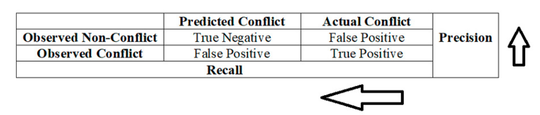
As discussed above, the study uses five classification algorithms: logistic, random forest, gradient boosting, SVM, and MLP. Metrics of accuracy, precision, and recall are used to evaluate model performance and estimate the gains in prediction for each algorithm used. Accuracy is a measure of the overall prediction accuracy or the proportions of correctly predicted outcomes. Precision (positive predictive values) is the percentage of results that are relevant (conflict). Recall (sensitivity) is the ratio of the true positive (TP) instances—in this case, conflict—that are correctly detected by the model. Recall is a measure of completeness, while precision is the measure of exactness. A model that has no false positive (FP) has a precision of 1 (100%), while a model with no false negative (FN) has a recall of 1 (100%).

$$Precision \left(PR\right)=\raisebox{1ex}{$TP$}\!\left/ \!\raisebox{-1ex}{$\left(TP+FP\right)$}\right.$$

$$Recall or Sensitivity \left(RC\right)=\raisebox{1ex}{$TP$}\!\left/ \!\raisebox{-1ex}{$\left(TP+FN\right)$}\right.$$

$$Accuracy=\raisebox{1ex}{$\left(TP+TN\right)$}\!\left/ \!\raisebox{-1ex}{$\left(TP+FP+TN+FN\right)$}\right.$$

For most researchers, there is a debate between which of these two measures can be used to assess the performance of the classification models: recall–precision, or the receiver operating characteristic (ROC) curve. Selecting between these two measures depends on the objective of the study. It is recommended that using the recall–precision measure is better when the predicted class is imbalanced [52]. Since our predictor variable, incidences of conflict, is imbalanced, we use the precision–recall measure.

It is important to note that there is a trade-off between recall and precision (Figure 1). Increasing model precision comes at the expense of recall. This implies that one has to find a balance between recall and precision. For this reason, F-score is also commonly used as a metric for evaluating a classifier performance. F-score is defined as the harmonic mean of precision and recall. A value closer to 1 implies that the classifier achieved a better combined precision and recall [43]. However, it is not always the case that balance is required by the modeler or end user. For example, if the modeler is interested in detecting conflict areas, a model providing 30 percent precision but 70 percent recall would be acceptable. This implies that although there may be a few incorrect alerts of conflict areas, the majority of conflict areas will be correctly identified [52].

Precision–recall curves are used to illustrate trade-offs between recall and precision. We have summarized this information into a single value called the average precision score (APS) (see [40]). The higher the APS, the better the score performs across these two measures. The APS is calculated from the precision–recall curve as the weighted mean precision achieved with an increase in recall at each threshold [40].

$$APS={{\displaystyle \sum }}_n\left(R{C}_n-R{C}_{n-1}\right)P{R}_n$$

Precision and recall are evaluated at the nth threshold along the curve.

5.2.1. Model Imbalance

Model imbalance can affect the predictive performance of a classification model. Since our data exhibits class imbalance, with much fewer observations reporting conflict compared to ones with no conflict, there is a tendency of classification models to emphasize the dominant class in estimates (no conflict class). If accuracy is the only measure that is used for assessment, the model might have a high accuracy rate but a low recall rate. For example, if 90 percent of our observations did not report conflict, and the model predicted that none of our observations had conflict, we would have close to a 90 percent accuracy rate. However, if the metric of interest is the recall rate, we need to increase the percentage of correctly predicted conflict cases and reduce false negatives. Providing balance (an equal number of negative and positive instances) in the training dataset can result in improved out-of-sample predictions on the test data [53].

Resampling is used to address the issue of imbalance in datasets. Over- and under-sampling might have both advantages and disadvantages. Over-sampling might lead to overfitting, while under-sampling might lead to discarding valuable information. In this study, we have used techniques proven to overcome these disadvantages. There are three popular techniques: (1) the synthetic minority over-sampling technique (SMOTE), which increases the minority class by introducing synthetic observations; (2) randomly under-sampling the majority class to match the minority class (NearMiss); and (3) randomly over-sampling the minority class until the counts of both classes match [53,54]. In our study, we have examined the performance of two popular resampling techniques—SMOTE and the ‘NearMiss’ algorithms [53,55]. The SMOTE draws a subset of the minority class, then generates additional similar synthetic observations; finally, it adds these observations to the original data [53]. The ‘NearMiss’ under-sampling algorithm uses Euclidean distance to select samples from the majority class. In the implementation of this algorithm in scikit-learn [40], there are three options: (1) selecting a majority class example with the minimum average distance to the three closest minority class examples; (2) selecting majority examples with the minimum average distance to three further minority class observations; and (3) selecting majority class examples with the minimum distance to each minority class observation. For this study, we used the technique that selects observations based on the minimum distance to the closest minority class observations [56].

5.2.2. Hyperparameter Tuning

In order to select the best predictive model, tuning the model over a range of hyperparameters is important. We used the fivefold cross-validation method, wherein the training data is split into five, of which four are used to train the model and one is held back for testing in a recursive approach [12]. We discuss the parameters tuned and the ranges of the parameters for each algorithm in detail in the Appendix A.

Since classification machine learning algorithms might not perform well if the variables are not normalized, we have used the in-built scikit-learn standard scaler to transform the continuous variables (missing values are imputed based on author understanding of the variable and data) [40]. The continuous variables were scaled, centered, and standardised with zero mean and unit variance. First, the algorithms were applied to transformed data without accounting for imbalance; next, imbalance was accounted for by over-sampling the dominant class; finally, imbalance was accounted for by under-sampling the dominant class. This is especially important from a policy perspective because “normalized” variables are easier to estimate and be predicated upon.

6. Results

6.1. Descriptive Statistics

There are 5928 observations and 119 predictor variables in our data. Of the observations, 7.9 percent reported an incidence of conflict in 2006, while 92.1 percent did not. This implies an imbalance since the majority reported no conflict. Therefore, the no-information rate for this imbalanced sample is 92.1 percent. Of the areas that reported conflict, over 55 percent reported an incident of conflict in the previous year (2005). The average conflict area was close to the capital and had a lower gross domestic product per capita (

Table 1. Descriptive statistics of conflict versus no-conflict areas.

Event	No Conflict (n = 5461)	Conflict (n = 467)
Past conflict	0.05 (0.22)	0.55 (0.49)
Presence of river	0.31 (0.46)	0.32 (0.46)
Industrial metals	0.08 (0.27)	0.19 (0.39)
Nightlight density	0.006 (0.04)	0.01 (0.04)
Area relying on rainfall and high inputs	4917.7 (10886)	8031.8 (17220)
Distance to capital city	542 (371)	487 (438)
Elevation level	89 (102)	148 (155)
GDP per capita	2310 (3238)	1310 (2249)
Area relying on rainfall and low inputs	4495 (11658)	7846 (15554)
Ruggedness of terrain	0.67 (0.89)	0.95 (1.12)
Maize	0.25 (0.43)	0.28 (0.45)
Malaria index	13.19 (9.4)	10.5 (8.2)

Source: based on author’s calculations. Note: mean values are reported in the table with standard deviations reported in parentheses.

).

The best models that generate a list of important predictor variables are the random forest and gradient boosting models. These will be discussed shortly.

6.2. Data Analysis

The results are presented as follows: first, we show the results of the model trained without adjusting for imbalance (

Table 2. Conflict prediction without adjusting for imbalance.

Model	Accuracy	Precision	Recall	F1 Score	Average Precision Score
Logistic Regression	0.934	0.694	0.351	0.466	0.296
Random Forest	0.927	0.923	0.124	0.128	0.218
Gradient Boosting	0.940	0.759	0.423	0.543	0.368
Multilayer perceptron	0.930	0.609	0.433	0.506	0.310
Support Vector Machines	0.935	0.885	0.237	0.374	0.272
No-information rate is 0.921

); then, we present the results after adjusting the conflict observations for imbalance using SMOTE and NearMiss under-sampling (

Table 3. Conflict prediction with adjustment using SMOTE.

Model	Accuracy	Precision	Recall	F1 Score	Average Precision Score
Logistic Regression	0.59	0.156	0.918	0.268	0.151
Random Forest	0.151	0.086	0.979	0.159	0.086
Gradient Boosting	0.082	0.082	1.00	0.151	0.082
Multilayer perceptron	0.79	0.224	0.619	0.329	0.17
Support Vector Machines	0.753	0.162	0.485	0.243	0.121

and

Table 4. Conflict prediction with adjustment using NearMiss technique.

Model	Accuracy	Precision	Recall	F1 Score	Average Precision Score
Logistic Regression	0.418	0.106	0.825	0.188	0.102
Random Forest	0.19	0.085	0.918	0.156	0.085
Gradient Boosting	0.328	0.1	0.897	0.179	0.098
Multilayer perceptron	0.588	0.125	0.67	0.21	0.111
Support Vector Machines	0.428	0.109	0.835	0.193	0.105

).

First, we are interested in exploring whether the prediction accuracy is above the no-information rate without performing any adjustment for imbalance. As Table 2 shows, prior to adjustment, all five models have a higher accuracy rate than the no-information rate of 92.1 percent, with the gradient boosting algorithm having the highest rate. The multilayer perceptron has the highest recall while the gradient boosting model the highest F1 score.

After training the model on a balanced sample using SMOTE and Nearmiss algorithms, the results indicate that, on average, SMOTE models have higher recall scores (Table 3 and Table 4).

Since models adjusted for imbalance using the SMOTE approach show better performance, we will focus our discussion on these results. The gradient boosting model has the highest recall, followed by the random forest and logistic models. The multilayer perceptron model has the highest F1 score, followed by the logistic and support vector machine models, respectively. The multi-perceptron model also has the highest average precision score, which indicates the best trade-offs between precision and recall along the precision–recall curve.

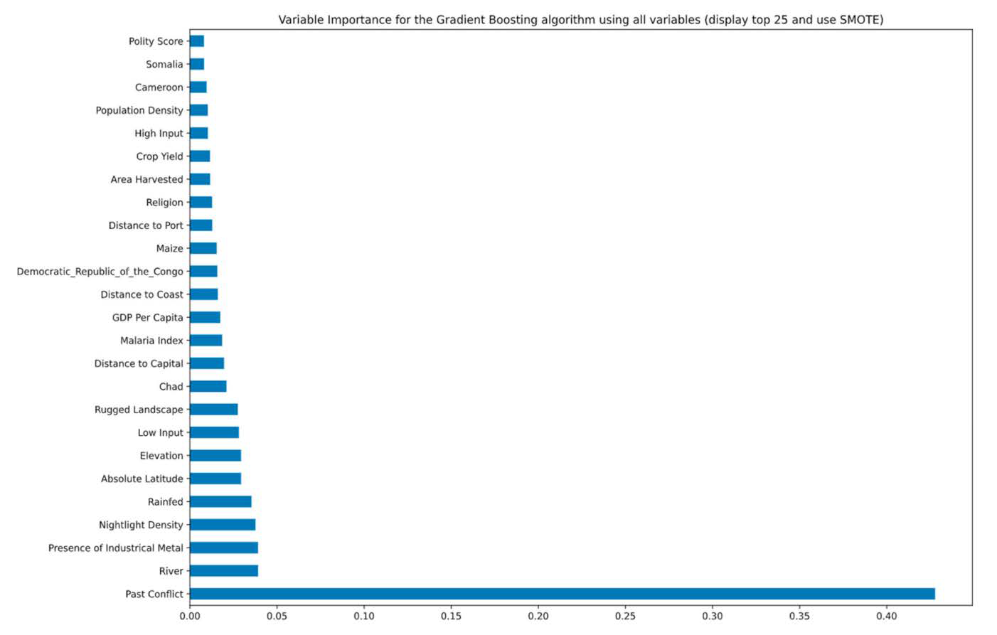
The model with the highest recall score, the gradient boosting algorithm, provides a ranking of the most important predictors that contribute to predicting conflict—past conflict, location near a river, the presence of industrial metals, density of night lights, and whether agriculture is rainfed or not. A list of 25 of the 119 variables in rank order are presented in Figure 2.

7. Discussion

Our study compares the logistic regression algorithm to machine learning algorithms in order to predict civil conflict in sub-Saharan Africa. This analysis creates a useful debate on which measure of prediction policymakers should prioritize—precision or recall—and how and when this choice would differ. In addition, this paper raises important questions as to why and when scientists should use ML approaches in the field of conflict assessment. Is it worthwhile to try and predict civil conflict with the new machine learning algorithms, given the available data? As such, our effort improves on the existing literature by collating a higher resolution dataset, adding gradient boosting mechanisms to the analysis and comprehensively comparing across several classification models while addressing issues of class imbalance.

The problem of class imbalance is ubiquitous in predicting conflict, wherein we observe disproportionately lower cases of conflict compared to ones without conflict. Correcting for issues of imbalance improves the performance of the algorithms—in particular, the recall scores. Modeling conflict data that has an imbalanced class problem creates two issues: (i) accuracy is not a good performance measure, and (ii) training a model using an imbalanced class may not provide good out-of-sample predictions where recall is a key metric for model evaluation. Using the models trained on an imbalanced dataset, our results indicate a higher accuracy rate than those trained using techniques that adjust from imbalance, SMOTE and NearMiss, but lower recall rates. The models trained on an imbalanced dataset have a high accuracy rate that is higher than the no-information rate in three algorithms, except for the support vector machines and gradient boosting. In the latter two, we see minimal increases to the no-information rate. This indicates that the accuracy rate is lower than the rate of the largest class (no conflict) in three models. Therefore, accuracy might not be a good measure for imbalanced classes, since it will be expected to have a high accuracy rate biased towards the majority class.

Our models are trained with future data to predict out-of-sample data. This approach mimics the real-world scenario of training current conflict to predict future data. Comparing performance across models, we found better predictions across all models for recall measures when imbalance was addressed compared to results where imbalance was not addressed. We have investigated two types of class imbalance learning methods—an over-sampling technique (SMOTE) and under-sampling technique (NearMiss). We found that although the results in terms of which algorithm performs best on precision, recall, and F1 score are similar, overall, the SMOTE technique provides better results on precision and recall on average. Focusing on the SMOTE technique results, we found that when the metric of interest is recall, gradient boosting outperforms all other algorithms; however, when the metric of interest is precision, multilayer perceptron provides the best results. Since recall is a critical metric in predicting and preventing conflict, where we are more interested in identifying all potential conflict areas, gradient boosting appears to be the best model for policymakers (a key drawback of the gradient boosting model is that it took three times as much time to train on a 16 GB RAM laptop than the other four algorithms. This implies that if time is an issue, random forest might be a second-best option). Another advantage of the gradient boosting model is that we can obtain a ranking of the most important variables (see Figure 2 for variable importance in predicting conflict). This not only improves our prediction of conflict but can also provide policymakers with guidance on which key predictors to collect data on in order to develop early warning systems. Not surprisingly, we have observed that past conflict is a critical predictor of future conflict. In addition, areas located near a developed city, which can be proxied with high night light density, is a good predictor of conflict. Another key predictor was the presence of industrial metals. The extant literature concerning sub-Saharan Africa has previously shown that the presence of minerals is a strong driver of conflict through extractive institutions.

From a policy perspective, our results emphasize the trade-offs between recall and precision in making appropriate decisions. On the one hand, a high recall measure is of importance since we prefer lower false negatives, i.e., identifying all areas with potential conflict. On the other hand, this implies that some areas that might be predicted as conflict zones will not observe conflict in reality, and any resources diverted to such areas will come at the cost of other, more fragile areas. The question then becomes whether it is important for the policymakers be informed of all potential areas that might experience conflict, even though the true outcome may be that conflict does not occur in some of the identified areas. Or would they rather ensure that most areas where conflict might occur are correctly predicted, with some areas being overlooked? This is the trade-off that policymakers need to assess depending on the existing infrastructure and available resources and on how much it might cost them to put in place preventative measures relative to the potential benefits.

Overall, we found that not all modern machine learning algorithms outperform the traditional logistic model. However, the ones that do so provide better performance across all metrics (recall and precision). When recall is the chosen measure, tree-based ML algorithms such as gradient boosting and random forest outperform the logistic regression algorithm; however, if we rank the balance using the F1 score, the logit model ranks among the top half of the five algorithms. If the policy goal is to minimize this trade-off, policymakers can consider selecting a balanced model with a high F1 score. However, if a modeler wants a balanced model with good precision and recall, then the multilayer perceptron algorithm provides the best model with a high F1 score. The trade-off with the multilayer perceptron that is similar with the SVM is that the model is like a black box. The model output provides predictions of performance metrics but does not indicate which variables are important in making that prediction. If understanding and examining the key predictor variables is of importance to the policymaker, then the best, most balanced model with SMOTE is the gradient boosting model, followed by the logit model. Therefore, given the discussed trade-offs in performance, we present all the recall and precision measures in our data that provide this information across all five models. This approach will enable the decision makers to choose the most appropriate model according to their goals and priorities.

8. Conclusions

In this paper, we have argued that given the availability of data, machine learning is the best way forward for policymakers to successfully predict and avert conflict. The alternative, causal inference models, is possible either by conducting randomized control trials (RCT) or defining a set of assumptions. Creating conflict scenarios for an RCT or examining verifiable conditions is neither ethical nor possible. Furthermore, a data-driven ML-based policy approach will not have to suffer from threats to identification that many econometric models encounter.

Until the recent past, research on violent conflict has primarily focused on generating correlations with sociopolitical and weather variables to imply causal inference through modeling finesse. However, as conflict datasets are becoming more disaggregated over time and information on the relevant variables are becoming richer, machine learning algorithms—both supervised and unsupervised—have been used in a few of the conflict studies to forecast and predict the onset of both local violence and war [13,14,30,31,33,35,57,58]. However, to our knowledge, this is among the first efforts that take advantage of continent-wide, big data and an even bigger set of carefully constructed variables of over 100 initial predictors, as well as comparing across multiple algorithms. We show a pathway to process intricate data with non-linear relationships and outperform maximum likelihood estimators in forecasting conflict onset. The ML algorithms have built-in “tuning”. In essence, tuning refers to model selection for data-driven algorithms that improve the performances of our models and enable us to be more systematic.

Our pragmatic approaches neither emphasize p-values nor identify deep-rooted causes of conflict in Africa. From the policymakers’ perspective, the associated coefficient or the average marginal effect of a variable is much less useful than the ability to predict the next conflict, along with some knowledge of its possible drivers. Hence, we plea to policymakers to maximize prediction performance by proposing empirical ways to make practical trade-offs. Instead of minimizing only in-sample error, our techniques aim to maximize out-of-sample prediction power. We acknowledge the limitations of the possible over-fitting issues of machine algorithms. However, we have also shed light on policy issues of whether to emphasize issues of precision or recall. Furthermore, we encourage policymakers not to be hesitant to commit type II errors in order to react quickly to prevent potential conflict. Our proposed approaches to the different machine learning algorithms as well logistic model presented can at least certainly be beneficial to preventing conflict events and assisting in achieving sustainable development. In addition, investment in data collecting and real-time access can enhance the application and delivery of good prediction models that can be obtained in a timely fashion and prove crucial to averting conflict. In recent times, the collection of sub-national-level conflict data has improved. New initiatives that stream real-time data can also benefit from our research. Our models can also be updated in real time to incorporate major early warning signs of conflict. Therefore, future studies should focus on how to develop and deploy algorithms that can provide timely recommendations. However, this needs to be a multi-stakeholder initiative since data collection and curation are costly ventures that can only be undertaken if funds are available and the stakeholders can expect a net benefit.