Adaptive Predictive Control with Neuro-Fuzzy Parameter Estimation for Microgrid Grid-Forming Converters

Abstract

Model predictive control (MPC) is a flexible and multivariable control technique with better dynamic performance than linear control. However, MPC is sensitive to parametric mismatches that reduce its control capabilities. In this paper, we present a new method of improving the robustness of MPC to filter parameter variations/mismatches by easily implementable parameter estimation. Furthermore, we extend the proposed technique for wider operating conditions by novel neuro-fuzzy estimation. The results, which are demonstrated by both simulations and real-time hardware-in-the-loop tests, show a steady-state parameter estimation accuracy of 95%, and at least 20% improvement in total harmonic distortion (THD) than conventional non-adaptive MPC under parameter mismatches up to 50% of the nominal values.

1. Introduction

Grid-forming converters hold an important place in microgrids powered by converter-interfaced renewable distributed energy resources (DERs). In AC microgrids, they have four necessary requirements, viz [1]: (1) During normal power system operations, they function as AC voltage sources. (2) During transient conditions arising from sudden power changes to the power system, they still operate as voltage sources, but observe safety limits for self-protection (e.g., current limits). (3) They can work without connection to the main grid, and provide voltage and frequency references to the network they operate in. (4) They could be required to provide black start services and grid restoration after a blackout; this would require supplementary energy storage.

The comprehensive requirements of grid-forming converters (hereafter called converters for simplicity) are difficult to achieve with conventional linear control techniques. For this reason, model predictive control (MPC), a robust, multi-variable control technique has been identified as a highly promising candidate for converters [2]. The performance of model predictive control is highly dependent on the accuracy of the prediction model of the controlled system. It has been shown that prediction errors are not only caused by parametric mismatches, but also by instantaneous values of load current and voltage—and this is dominantly manifest with inductance mismatches and negligible with resistive mismatches [3]. Thus, whenever mismatches occur between the system parameter values utilized in the model (nominal values) and the actual/physical values, it results in control errors. These errors manifest as persistent steady-state offsets [4] and distorted output signals [5]; these even deteriorate further in transient situations. Other factors that cause model mismatches include temperature, measurement errors, operational time of use of the equipment/electronics, etc. The methods to address the MPC-based parameter accuracy errors are grouped as model-free, disturbance estimation, and adaptive model techniques.

Model-free methods do not require a prior knowledge of the plant [6,7,8], but their accuracy is determined by the sampling frequency [9,10]. In addition, some of them (including Kalman filter, deadbeat, sliding mode, least-square-based) have utilized complex and computationally-intensive algorithms or require extra measurements [11,12]. Disturbance estimation methods estimate the disturbance caused by parameter mismatches and uncertainties, and provide a feedforward compensation [13,14]. Adaptive parameter predictive control (which is less computationally demanding) utilizes an online estimate of the actual parameter in the prediction model, and this results in more accurate controls [5,15]. Nonetheless, there are few investigations on adaptive predictive control, and existing solutions are constrained by the limited range of the operational application.

The robustness and accuracy of MPC can be improved with online parameter estimation. This reduces the errors that arise from mistmatch between physical and control model parameter values. In [16], the estimation of inductance and resistance was reported for the voltage-oriented control of three-phase pulse-width modulated (PWM) rectifiers, but it required significant tuning efforts for the adaptive rate. A Lyapunov-based estimation of inductance for a model reference adaptive system reported in [17], aided the improvement in line voltage estimation accuracy for an active front-end (AFE) rectifier. Several estimation methods are focused on the application to balanced grid conditions, e.g., the least square method in [18]. The authors of [19,20] investigated inductance estimation (by gradient correction and Kalman filter) under distorted grid conditions. The proposed solutions reduced both harmonics and ripples but with a high computational burden.

In recent times, power electronics researchers have sought to explore data-based methods as alternatives to model-based techniques [21,22]. Some benefits reported in the literature are the improvement of reliability (sensor reduction) [23,24], and reduction of hardware requirements [25]. One artificial intelligence (AI) data-based method is neuro-fuzzy control, and it is a hybrid of fuzzy logic and artificial neural networks (ANN) [26]. The membership functions used in a fuzzy controller can be auto-tuned (with a higher degree of accuracy than heuristic techniques) by offline ANN training done with historical input-output data of the plant. Although the neuro-fuzzy controller has an increasing computational burden as the fuzzy subsets increase, it has the advantage of being operable over a wider range of operating conditions than conventional controllers [27]. Hence, an optimal trade-off between accuracy and cost is done in applications to converter control for microgrids [28] and electrical drives [29,30].

The above literature review indicates that auto-tuned parameter estimation can improve predictive control’s robustness to parameter variation/mismatch. Moreover, the neuro-fuzzy method, which is a hybrid of expert-knowledge and data-based design, is yet to be applied to either microgrid parameter estimation or MPC. Furthermore, many of the proposed solutions operate around a specific operating point, requiring re-tuning with a change in operating conditions. Motivated by these, this paper proposes novel parameter auto-tuning for MPC using two methods. First, a simple estimation procedure for a specific operating point and second, a neuro-fuzzy based estimation of parameter variation that can cover a wider operational range. Please note that the estimation being proposed in this control scheme is the estimation of the amount of filter parameter (L or C) variation relative to its pre-known nominal value. The major contributions of this work are highlighted as follows:

• We present a theoretical analysis of LC-filter parameter variation dynamics (Section 3.1);
• To extend the operational range of the estimator, we introduce a new neural–trained fuzzy logic parameter estimator for islanded AC microgrids (Section 4.2);
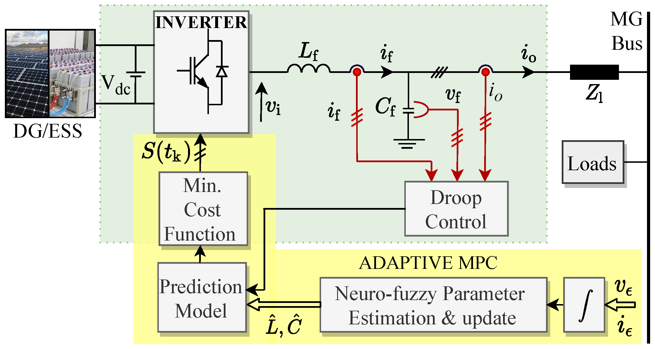
• The new estimator is then embedded in a comprehensive adaptive predictive control scheme for microgrid converters (Section 3). The overall scheme has much better performance than a conventional MPC under parametric mismatches, with results verified via extensive simulations and hardware-in-the-loop (HiL) experiments.

The organization of the paper comprises the introduction of MPC for converters in Section 2, the underlying principles of an adaptive neuro-fuzzy control in Section 4, and the proposed adaptive MPC control schemes in Section 3. The results and conclusion are provided in Section 5 and Section 6 respectively.

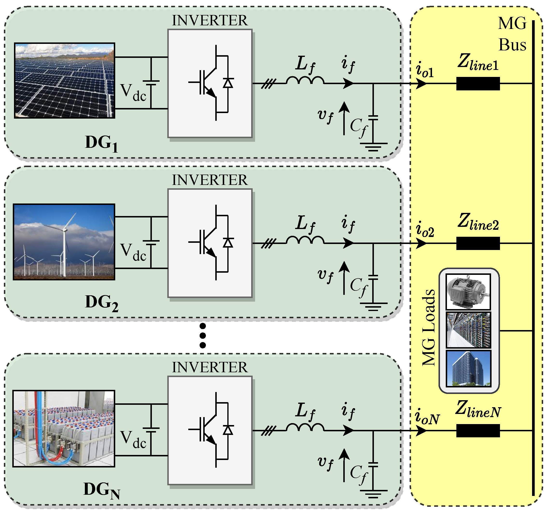
2. Conventional Dual-Objective Model Predictive Inverter Control

An AC microgrid with inverter-interfaced distributed generation and common AC loads is shown in Figure 1. This section will introduce the fundamental principles for the predictive control of inverters, as a basis for later developing the proposed adaptive MPC system in Section 3.

2.1. LC Filter

Assuming the inverter in Figure 1 has identical filter parameter values in all three phases (i.e., inverter legs), we invoke Clarke’s transformation to obtain the $\alpha \beta$ transformation of the three-phase current and voltage vectors:

$$x_{\alpha }+j{x}_{\beta }=\mathbf{K}{\left(\begin{array}{ccc}{x}_{\mathrm{a}}& x_{\mathrm{b}}& x_{\mathrm{c}}\end{array}\right)}^{\prime },$$

(1)

where $\mathbf{K}=\frac{1}{3}$ $\left(\begin{array}{ccc}1& e^{j\frac{2}{3}\pi }& e^{j\frac{4}{3}\pi }\end{array}\right).$ By Kirchoff’s current and voltage laws, the LC filter is modeled in continuous-time state-space as:

$$\frac{d}{dt}\left(\begin{array}{c}{i}_{\mathrm{f}}\\ v_{\mathrm{f}}\end{array}\right)=\mathbf{A}\left(\begin{array}{c}{i}_{\mathrm{f}}\\ v_{\mathrm{f}}\end{array}\right)+\mathbf{B}\left(\begin{array}{c}{v}_{\mathrm{i}}\\ i_{\mathrm{o}}\end{array}\right),$$

(2)

where $\mathbf{A}=\left[\begin{array}{cc}-\frac{R_{\mathrm{f}}}{L_{\mathrm{f}}}& -\frac{1}{L_{\mathrm{f}}}\\ \frac{1}{C_{\mathrm{f}}}& 0\end{array}\right];$ $\mathbf{B}=\left[\begin{array}{cc}\frac{1}{L_{\mathrm{f}}}& 0\\ 0& -\frac{1}{C_{\mathrm{f}}}\end{array}\right].$ The variables $R_{\mathrm{f}},L_{\mathrm{f}},\mathrm{and}{C}_{\mathrm{f}}$ represent the filter resistance, inductance, and capacitance respectively. The filter current is $i_{\mathrm{f}}=i_{\mathrm{f}\alpha }+j{i}_{\mathrm{f}\beta }$; the filter voltage is $v_{\mathrm{f}}=v_{\mathrm{f}\alpha }+j{v}_{\mathrm{f}\beta }$; the inverter output voltage is $v_i=v_{\mathrm{i}\alpha }+j{v}_{\mathrm{i}\beta }$; and the load current is $i_{\mathrm{o}}=i_{\mathrm{o}\alpha }+j{i}_{\mathrm{o}\beta }$.

The discrete-time state space model of Equation (2) is achieved using zero-order-hold (ZOH) with a sampling period $T_s$, and to account for digital computational delays, the two-step-forward prediction is employed as:

$$\left(\begin{array}{c}{i}_{\mathrm{f}}^{\mathrm{p}}(k+2)\\ v_{\mathrm{f}}^{\mathrm{p}}(k+2)\end{array}\right)={\mathbf{A}}_{\mathbf{d}}\left(\begin{array}{c}{i}_{\mathrm{f}}(k+1)\\ v_{\mathrm{f}}(k+1)\end{array}\right)+{\mathbf{B}}_{\mathbf{d}}\left(\begin{array}{c}{v}_{\mathrm{i}}(k+1)\\ i_{\mathrm{o}}(k+1)\end{array}\right),$$

(3)

where ${\mathbf{A}}_{\mathbf{d}}=e^{\mathbf{A}{T}_s}$ and ${\mathbf{B}}_{\mathbf{d}}={\int }_0^{T_s}{e}^{\mathbf{A}\tau }\mathbf{B}d\tau$. In practice, the load current $i_{\mathrm{o}}$ is of slow dynamics (grid frequency); thus it can be assumed constant within two samples ($i_{\mathrm{o}}(k+1)\approx i_{\mathrm{o}}\left(k\right)$), without any loss of accuracy.

2.2. Cost Function

Minimizing the Euclidean distance error of tracking both $i_{\mathrm{f}}$ and $v_{\mathrm{f}}$ will yield more accurate results than tracking either alone due to the cross-coupling between them (see Equation (2)). The cost function in Equation (4) achieves the dual-objective tracking.

$$\begin{gathered} G_{\mathrm{c}}={\parallel v_{\mathrm{f}}^{*}-v_{\mathrm{f}}(k+2)\parallel }^2+{\chi }_{\mathrm{i}}{\parallel i_{\mathrm{f}}^{*}-i_{\mathrm{f}}(k+2)\parallel }^2 \\ +{\chi }_{\mathrm{u}}{u}_{\mathrm{sw}}^2(k+2)+{\psi }_{\lim }(k+2), \end{gathered}$$

(4)

where ${\chi }_{\mathrm{i}}$ is the current term weighting factor, ${\chi }_{\mathrm{u}}$ penalizes the switching effort $u_{\mathrm{sw}}\left(k\right)=\sum |u\left(k\right)-u(k-1)|$, and the fourth term accounts for the physical current limits on the device as:

$${\psi }_{\lim }\left(k\right)=\left\{\begin{array}{cc}0\hfill & \mathrm{if}|i_{\mathrm{f}}\left(k\right)|\le i_{\max },\hfill \\ \infty \hfill & \mathrm{if}|i_{\mathrm{f}}\left(k\right)|>i_{\max }.\hfill \end{array}\right.$$

(5)

Equation (6) defines the reference voltage, where $V_{\mathrm{ref}}$, ${\omega }_{\mathrm{ref}}$ are the reference voltage amplitude and angular frequency respectively:

$$v_{\mathrm{f}}^{*}=V_{\mathrm{ref}}\cos \left({\omega }_{\mathrm{ref}}t\right)+j{V}_{\mathrm{ref}}\sin \left({\omega }_{\mathrm{ref}}t\right).$$

(6)

The reference current is given by [31]:

$$i_{\mathrm{f}}^{*}=(C_{\mathrm{f}}{\omega }_{\mathrm{ref}}{v}_{\mathrm{f}\beta }^{*}+i_{\mathrm{o}\alpha })-j{C}_{\mathrm{f}}{\omega }_{\mathrm{ref}}{v}_{\mathrm{f}\alpha }+j{i}_{\mathrm{o}\beta }.$$

(7)

2.3. Droop Relationship

The droop curve dictates how power drawn by the common load is shared between parallel connected inverters and is given by the following equations:

$$\omega ={\omega }^{*}-k_{\mathrm{p}}(\tilde{P}-P^{*}),$$

(8)

$$V=V^{*}-k_{\mathrm{q}}(\tilde{Q}-Q^{*}),$$

(9)

where $k_{\mathrm{p}}$ and $k_{\mathrm{q}}$ are MG droop coefficients for frequency-active-power and voltage-reactive-power respectively.

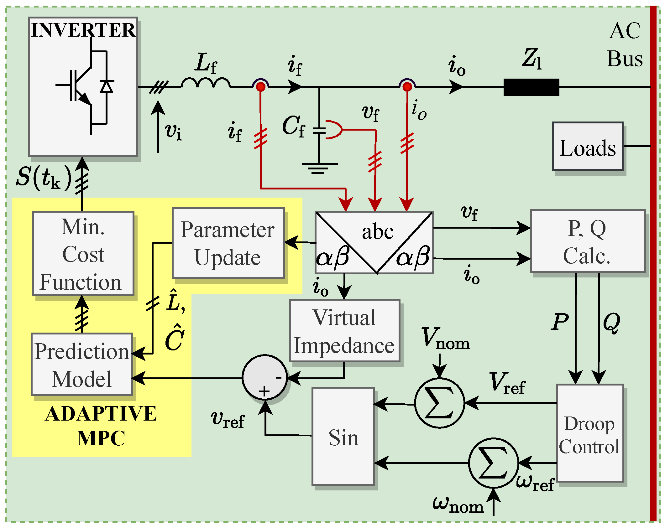
3. The Proposed Adaptive MPC Scheme

In this section, a new parameter variation estimation method will first be introduced; next, its application to predictive control will be illustrated.

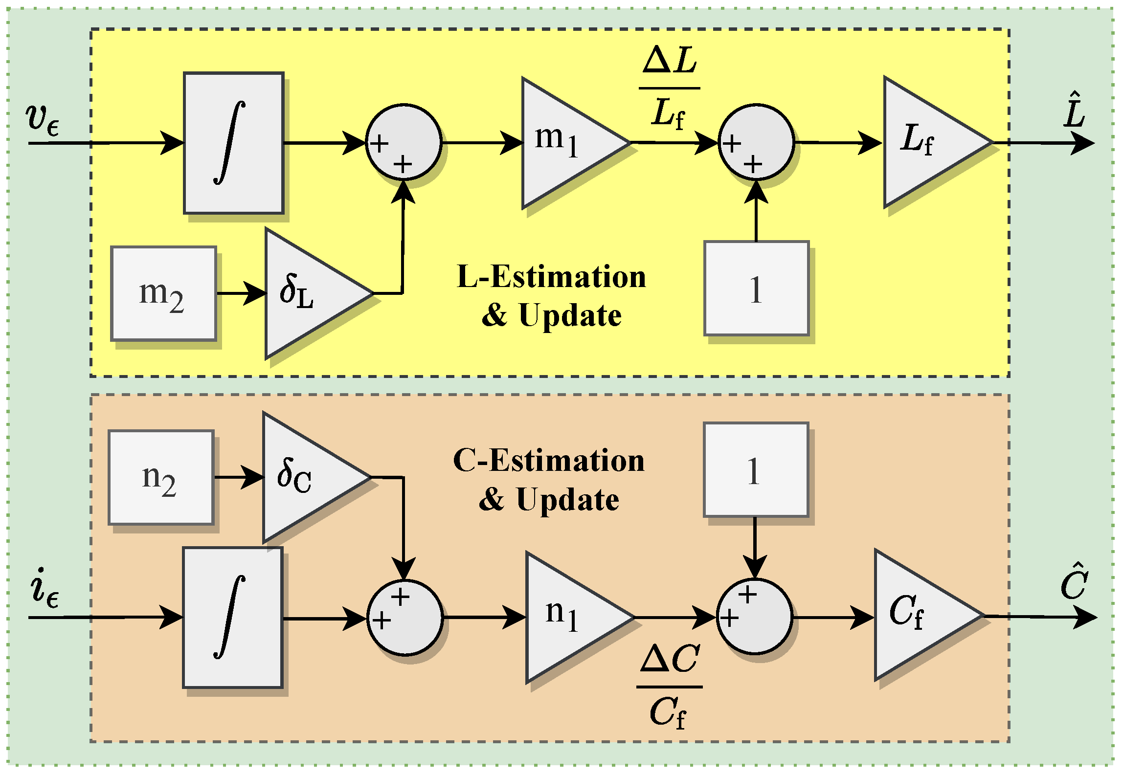
3.1. Parameter Estimation and Adaptive Model Update

The proposed adaptive MPC scheme is described by Figure 2. The main difference between this scheme and the conventional scheme is that the output current, filter current, and voltage are utilized to first estimate the variation in the filter inductance and capacitance from their nominal values $L_{\mathrm{f}}$ and $C_{\mathrm{f}}$, respectively. Since MPC’s prediction errors from parametric mismatches are negligible for resistive mismatches and dominant in passive energy-storage elements [3], this study attends only to inductive and capacitive mismatches/variations from their nominal values. We define ${\delta }_{\mathrm{y}}$ to indicate the sign of the parameter mismatch relative to the nominal value. ${\delta }_{\mathrm{y}}$$\forall y\in [C,L]$ as:

$${\delta }_{\mathrm{y}}=\left\{\begin{array}{cc}-1\hfill & \mathrm{if}\Delta y_{\mathrm{f}}\mathrm{is}\mathrm{positive},\hfill \\ +1\hfill & \mathrm{if}\Delta y_{\mathrm{f}}\mathrm{is}\mathrm{negative}.\hfill \end{array}\right.$$

(10)

3.1.1. Inductance Variation Estimation

With reference to Figure 5, the difference between the voltage at the inverter output $v_i$ and the voltage across the filter capacitor $v_{\mathrm{f}}$ is linearly proportional to the rate of change of inductor current $i_{\mathrm{f}}$. Therefore, when there is an inductance variation $\Delta L$, the instantaneous voltage difference ($v_i-v_{\mathrm{f}}$) relative to the voltage difference at the nominal inductance $L_{\mathrm{f}}$ is described by:

$$v_{ϵ}=(v_{\mathrm{i}}-v_{\mathrm{f}}){{|}_{[L_{\mathrm{f}}+\Delta L]}-(v_{\mathrm{i}}-v_{\mathrm{f}})|}_{L_{\mathrm{f}}}=\Delta L\frac{d{i}_{\mathrm{f}}}{dt}.$$

(11)

After algebraic operations as explained in Appendix A.1, the normalized capacitance variation becomes:

$$\frac{\Delta L}{L_{\mathrm{f}}}=m_1\left(\int v_{ϵ}\left(t\right)+m_2{\delta }_{\mathrm{L}}\right),$$

(12)

where $m_1=1/\left(L_{\mathrm{f}}{i}_{\mathrm{f}\_\mathrm{amp}}\right)$ and $m_2$ is a tuned coefficient, $i_{\mathrm{f}\_\mathrm{amp}}$ is the amplitude of $i_{\mathrm{f}}$, $v_{ϵ}=(v_{\mathrm{i}}-v_{\mathrm{f}}){{|}_{[L_{\mathrm{f}}+\Delta L]}-(v_{\mathrm{i}}-v_{\mathrm{f}})|}_{L_{\mathrm{f}}}$, and ${\delta }_{\mathrm{L}}$ is as defined in (10).

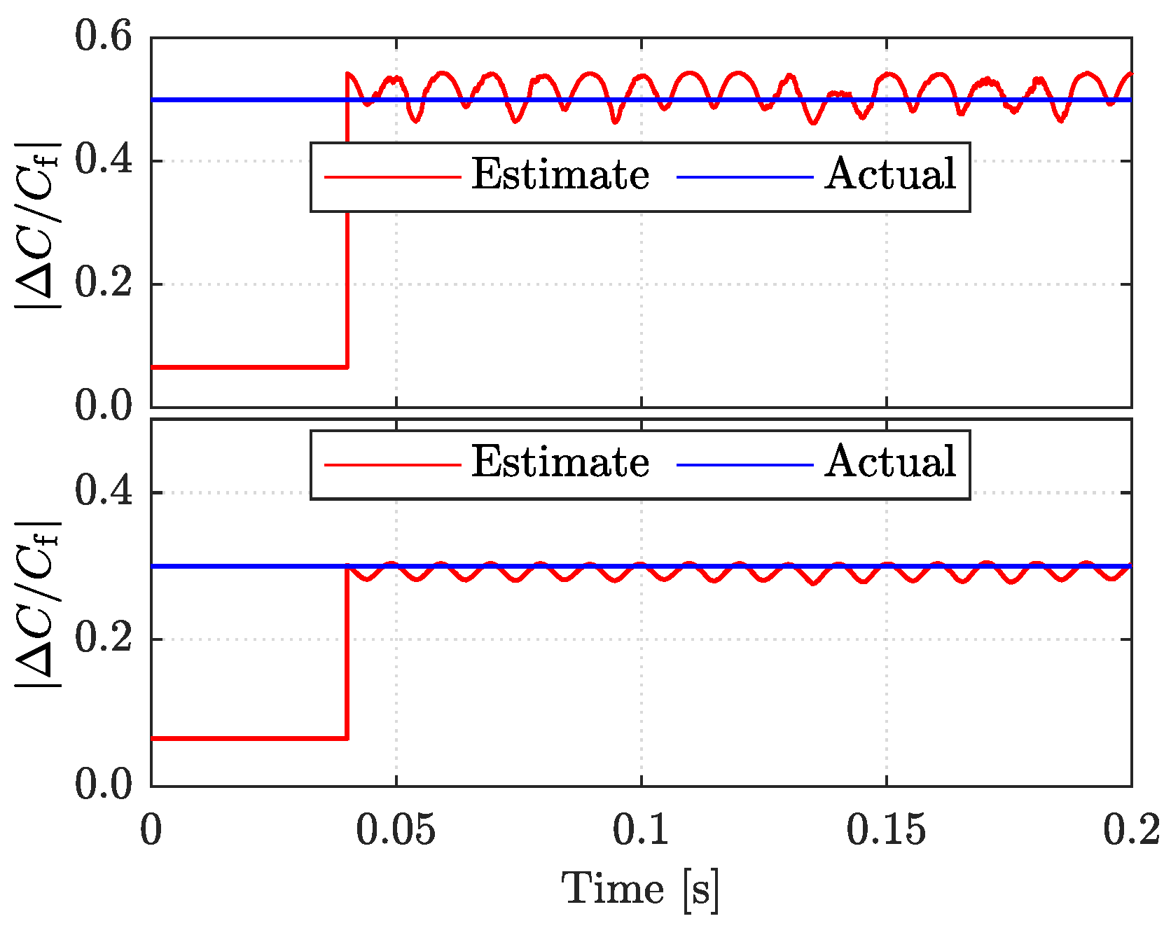
3.1.2. Capacitance Variation Estimation

The capacitance variation dynamics is:

$$i_{ϵ}=(i_{\mathrm{f}}-i_{\mathrm{o}}){{|}_{[C_{\mathrm{f}}+\Delta C]}-(i_{\mathrm{f}}-i_{\mathrm{o}})|}_{C_{\mathrm{f}}}=\Delta C\frac{d{v}_{\mathrm{f}}}{dt}.$$

(13)

Hence, the normalized capacitance variation is determined by the linear relationship in Equation (14). After algebraic operations as explained in Appendix A.2, the normalized capacitance variation becomes:

$$\frac{\Delta C}{C_{\mathrm{f}}}=n_1\left(\int i_{ϵ}\left(t\right)+n_2{\delta }_{\mathrm{C}}\right),$$

(14)

where $n_1=1/\left(C_{\mathrm{f}}{v}_{\mathrm{f}\_\mathrm{amp}}\right)$ and $n_2$ is a tuned coefficient, $v_{\mathrm{f}\_\mathrm{amp}}$ is the amplitude of $v_{\mathrm{f}}$, and $i_{ϵ}=(i_{\mathrm{f}}-i_{\mathrm{o}}){{|}_{[C_{\mathrm{f}}+\Delta C]}-(i_{\mathrm{f}}-i_{\mathrm{o}})|}_{C_{\mathrm{f}}}$, and ${\delta }_{\mathrm{C}}$ is as defined in (10).

3.2. Adaptive Model Update

Equations (10)–(14) together define how the proposed adaptive estimation method gives the estimated parameter $\widehat{y}$ at the kth sampling instant as:

$$\widehat{y}\left(k\right)=y_{\mathrm{f}}\left(1+\frac{\Delta y\left(k\right)}{y_{\mathrm{f}}}\right)\forall y\in [C,L],$$

(15)

and this is illustrated in Figure 3.

The estimated variations $\frac{\Delta L}{L}$ and $\frac{\Delta C}{C}$ are processed using the adaptive estimator in Figure 3 to generate the updated inductance $\widehat{L}$ and updated capacitance $\widehat{C}$ respectively. This is done for every sample. The updated parameters are used to compute the state-space matrices $\mathbf{A}$ and $\mathbf{B}$ whose terms are needed to predict the values of $i_{\mathrm{f}}^{\mathrm{p}}$ and $v_{\mathrm{f}}^{\mathrm{p}}$.

After the parameters have been updated as described by Equation (15), they are used to update the system matrices as:

$$\widehat{\mathbf{A}}=\left[\begin{array}{cc}-R_{\mathrm{f}}/\widehat{L}& -1/\widehat{L}\\ -1/\widehat{C}& 0\end{array}\right],\widehat{\mathbf{B}}=\left[\begin{array}{cc}1/\widehat{L}& 0\\ 0& -1/\widehat{C}\end{array}\right].$$

(16)

The prediction model in (3) becomes modified to:

$$\left(\begin{array}{c}{i}_{\mathrm{f}}^{\mathrm{p}}(k+2)\\ v_{\mathrm{f}}^{\mathrm{p}}(k+2)\end{array}\right)={\widehat{\mathbf{A}}}_{\mathbf{d}}\left(\begin{array}{c}{i}_{\mathrm{f}}(k+1)\\ v_{\mathrm{f}}(k+1)\end{array}\right)+{\widehat{\mathbf{B}}}_{\mathbf{d}}\left(\begin{array}{c}{v}_{\mathrm{i}}(k+1)\\ i_{\mathrm{o}}(k+1)\end{array}\right),$$

(17)

where ${\widehat{\mathbf{A}}}_{\mathbf{d}}=e^{\widehat{\mathbf{A}}{T}_s}$ and ${\widehat{\mathbf{B}}}_{\mathbf{d}}={\int }_0^{T_s}{e}^{\widehat{\mathbf{A}}\tau }\widehat{\mathbf{B}}d\tau$. The cost function in (4) still applies.

4. The Proposed Neuro-Fuzzy Parameter Estimator

In this section, the principles underlying adaptive neuro-fuzzy control will be introduced as a foundation for application to the proposed parameter estimation scheme.

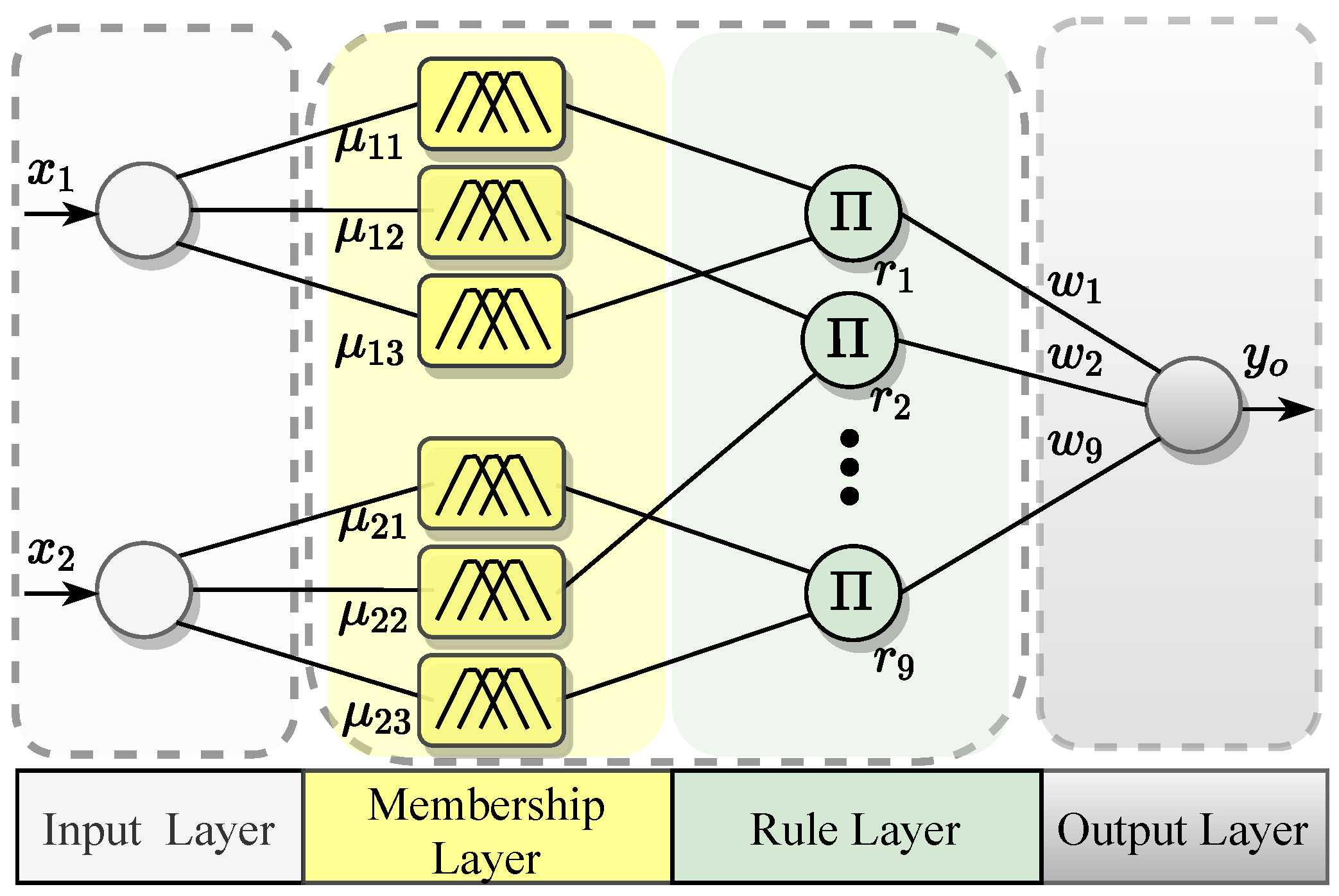
4.1. Principles of Adaptive Neuro-Fuzzy Control

A neuro-fuzzy control system combines the principles of fuzzy systems and artificial neural networks (ANN) to regulate the relationship between inputs and outputs. In general, ANN is applied to improve the accuracy of an initially-designed fuzzy controller according to historical data, and this will be further explained in the following discussion. Figure 4 shows the outlay of this paper’s neuro-fuzzy scheme. It comprises four layers: Input layer, membership layer, rule layer, and the output layers [32,33].

4.1.1. The Input Layer

Comprises inputs $x_1,x_2$. In this study, the inputs are the inductance variation dynamics $v_{ϵ}$ and capacitance variation dynamics $i_{ϵ}$, as defined in Equations (11) and (13) respectively.

4.1.2. The Membership Layer

Fuzzifies the input variables by converting them to numbers ranging from 0 to 1 through membership functions. Membership functions are user-defined curves used to analyze/map the fuzzy system’s input data. The generalized bell-shaped membership function is used in this study, and is defined as $f(x,a,b,c)={\left[1+{∥\frac{x-c}{a}∥}^{2b}\right]}^{-1}$, where a determines the width of curve, b defines the shape of the curve on either side, and c is the center of the membership function.

4.1.3. The Rule Layer

Multiplies the input signals as in Equation (18), to give $l_r$, where $w_{\mathrm{ij}}$ is the weight between membership and rule layers, taken as one, ${\mu }_{ij}$ is membership function i with neighbor j, for each input $x_{\mathrm{i}}$.

4.1.4. The Output Layer

In this case is a single node that computes results as in Equation (18), where $w_{\mathrm{ij}}$, ${\mu }_{ij}$, and $x_{\mathrm{i}}$ are as earlier defined, $N_r$ is the total number of rules, and $N_{\mathrm{mf}}$ is the total number of membership functions [32,33]:

$$y=\sum _{r=1}^{N_r}{w}_r\underset{:=l_r}{\underbrace{\prod _{i=1}^{N_{\mathrm{mf}}}{w}_{\mathrm{ij}}{\mu }_{\mathrm{ij}}\left(x_{\mathrm{ij}}\right)}}.$$

(18)

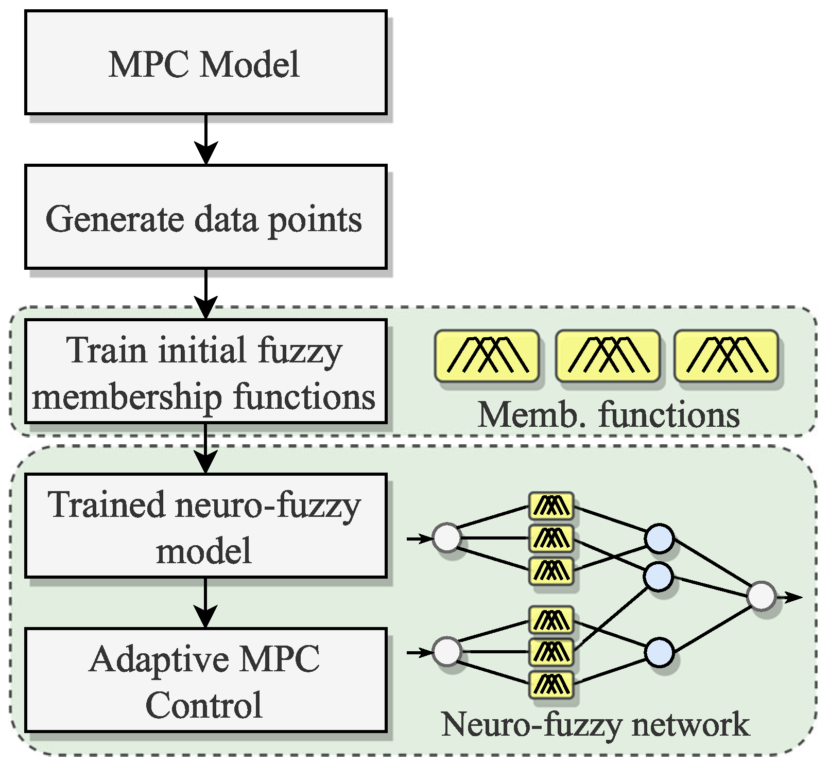
4.2. Neuro-Fuzzy Parameter Estimation

Due to its adaptability to a wide range of operating conditions, we propose the following neuro-fuzzy parameter estimation scheme, which follows from preceding discussions. The earlier defined parameter variation dynamics $v_{ϵ}$ and $i_{ϵ}$ are necessary inputs for the neuro-fuzzy estimator. The overall structure of the control scheme is shown in Figure 5. It comprises a four-leg, H-bridge, three phase inverter whose switching is dictated by the adaptive MPC scheme that will be further described below. The LC-filter voltage and current variation dynamics ($v_{ϵ}$ and $i_{ϵ}$ respectively, earlier defined in Equations (11) and (13)) are fed into the neuro-fuzzy parameter estimation and update block; an integrator is used to smoothen the signals by filtering high frequency components. After the neural-network-based training of membership functions, the estimation block accurately estimates parameter mismatches ($\Delta L$ and $\Delta C$) to a maximum mean square error less than 5%. Thus the updated parameters for the prediction model are $\widehat{L}=L_{\mathrm{f}}+\Delta L$ and $\widehat{C}=C_{\mathrm{f}}+\Delta C$.

The workflow to achieve the trained neuro-fuzzy estimator is shown in Figure 6. About seven million data points were generated with the conventional MPC model while the nominal filter parameters where increased in linear scales of 10% up to 50%. For instance for the inductance, we had $L_{\mathrm{f}}$ to $0.5L_{\mathrm{f}}$. This was done for events including load step changes too. The data were then used to train the initial membership functions created (see Figure 7a). Details on rules regarding selections of appropriate membership functions are outside the scope of this paper, but can be found in [33]. The initial membership functions were designed with MATLAB Simulink Fuzzy Logic Toolbox by expert knowledge of the system, in such a manner that they model the relationship between input and output signals (here, the input signals are $v_{ϵ}\mathrm{and}{i}_{ϵ}$, and the output signals are $\Delta L\mathrm{and}\Delta C)$. As earlier mentioned in Section 4, the bell-shaped membership functions were used here (Figure 7a). These were then trained offline, using MATLAB Simulink’s Neuro-Fuzzy Toolbox, for improved accuracy with the system’s input-output data from simulation runs, resulting in the trained functions shown in Figure 7b. The trained system had 4.2 million training data pairs, 2.5 million checking data pairs, 35 nodes, 9 linear parameters, 18 nonlinear parameters, and 9 fuzzy rules.

5. Results and Discussion

The simulative and real-time hardware-in-the-loop results are presented in this section. The discussion is done under headings of system description, parameter estimation, transient performance, steady-state performance, and parametric robustness.

5.1. System Description

The proposed control scheme was tested via both simulations and HiL demonstrations. The overall system topology and control scheme are depicted in Figure 2, and the system parameters are provided in

Table 1. Parameters of the test microgrid system.

Parameters	Symbols	Values
DC voltage	$V_{\mathrm{dc}}$	650 V
Nominal frequency	$f_{\mathrm{nom}}$	50 Hz
Nominal voltage	$V_{\mathrm{nom}}$	250 V
Filter	$R_{\mathrm{f}}$$L_{\mathrm{C}};$$C_{\mathrm{f}}$	$R_{\mathrm{f}}=0.05\Omega$ $L_{\mathrm{f}}=2$ mH, $C_{\mathrm{f}}=80$μF
Sampling time	$T_s$	$25$μs (Simulation) $10$μs (HiL controller) $7$μs (HiL plant discretization)
Droop coefficients	$m_{\mathrm{p}}$, $m_{\mathrm{q}}$	$m_{\mathrm{p}}=25$μV/W, $m_{\mathrm{q}}=50$μrad/sVar
Line impedance	$R_{\mathrm{l}}$, $L_{\mathrm{l}}$	$R_{\mathrm{l}}=0.1\Omega$, $L_{\mathrm{l}}=2.4$ mH
Virtual impedance	$R_{\mathrm{v}}$, $L_{\mathrm{v}}$	$R_{\mathrm{v}}=0.2\Omega$, $L_{\mathrm{v}}=4$ mH

. The simulation tests were carried out with MATLAB/Simulink software, while the real-time HiL tests were done with two PLECS RT-Box 1 real-time systems which exchange digital pulse-width modulation and analog signals: One for the controller, and the other for the plant subsystem. The laboratory testbench is shown in Figure 8.

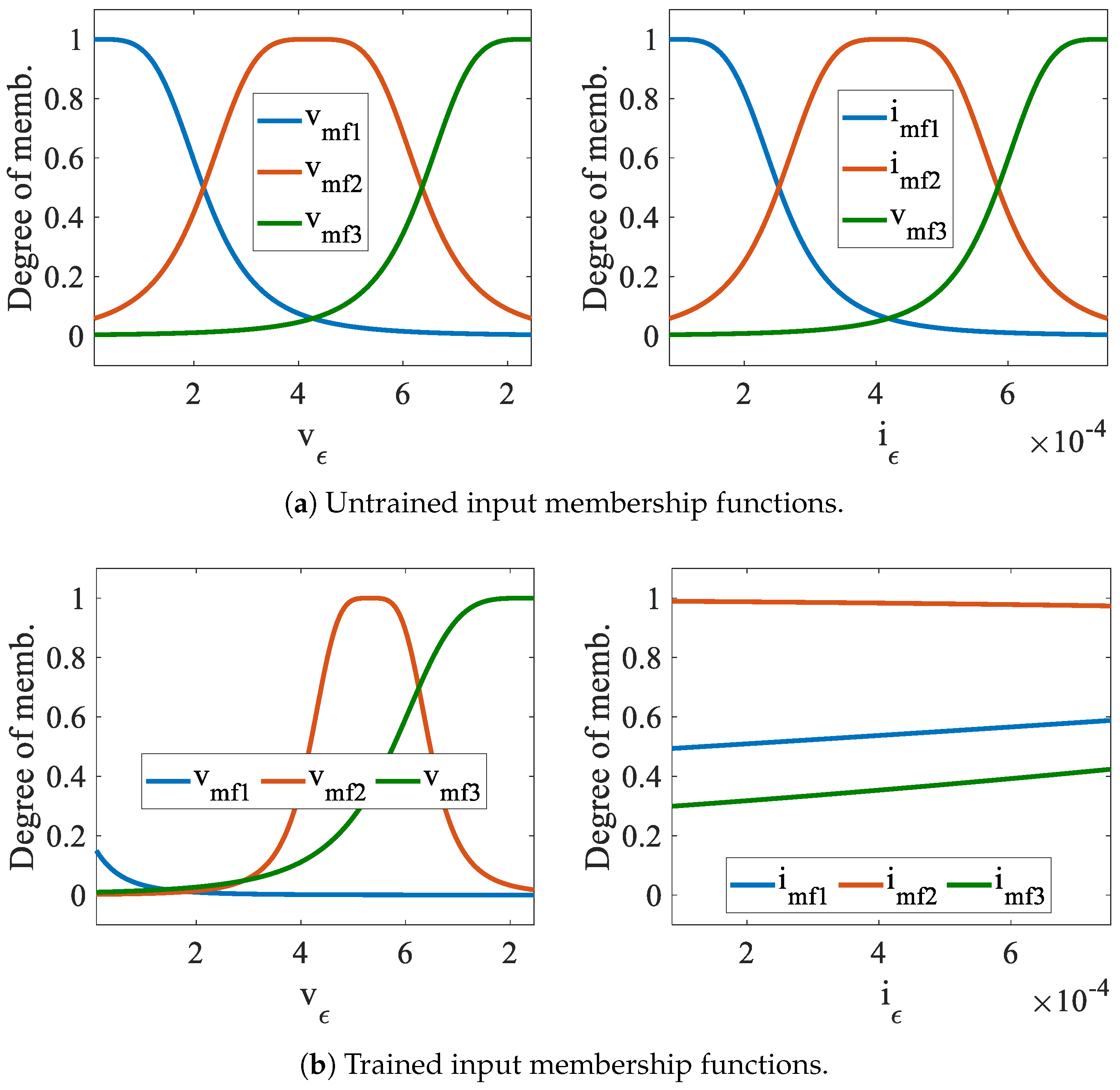
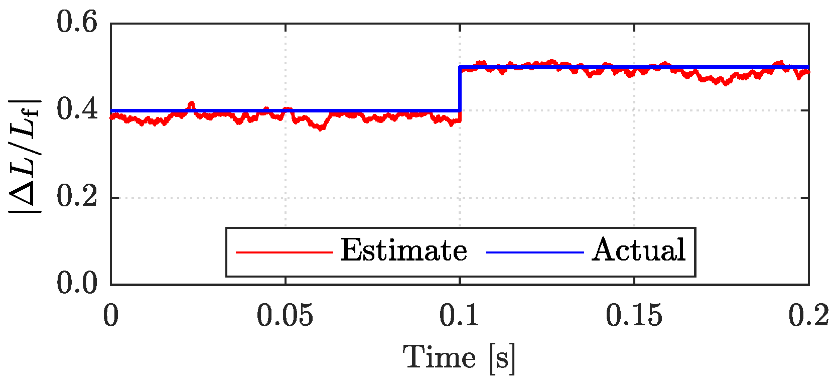
5.2. Parameter Estimation

Both parameter estimation methods earlier described in Section 3 and Section 4 have identical levels of accuracy. Therefore, for the simulation results in this section, only results for the neuro-fuzzy parameter variation estimation are shown. Figure 9 shows the estimation results for filter capacitance. The designed estimator was able to detect the deviation from the nominal values with a high degree of accuracy. The capacitance estimation has ripples that are higher as the mismatch with nominal grows. Similarly, inductance estimation results are illustrated in Figure 10, and it is observed that for both values tested, the estimator came within a high degree of accuracy. The mean square training and checking errors during the neuro-fuzzy training process were 4.73% and 4.12% respectively. In addition, higher training error values were observed with load step change data—as high as 11.5%. For parameter estimation errors less than 10%, identical power quality as using the actual values is obtainable.

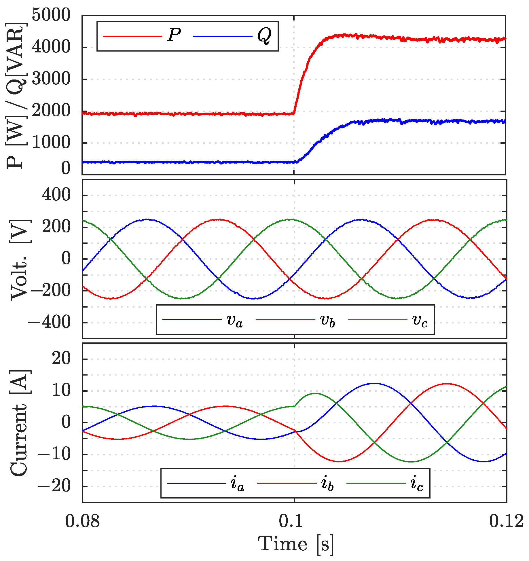
5.3. Neuro-Fuzzy Transient Performance

Figure 11 is a plot of the simulated performance of the proposed neuro-fuzzy-based estimation and adaptive MPC control with a step chanve in active and reactive powers. During the transient operation, rapid and robust transient responses are desired, and these were achieved using the adaptive neuro-fuzzy MPC scheme in Figure 5. Figure 11 shows that during the transient period (initiated at 0.1s), the proposed control scheme did not lose tracking performance, the voltage ripples are very low, while transient distortions are minimized, due to the effective parameter estimation and compensation for the mismatch in the inductance.

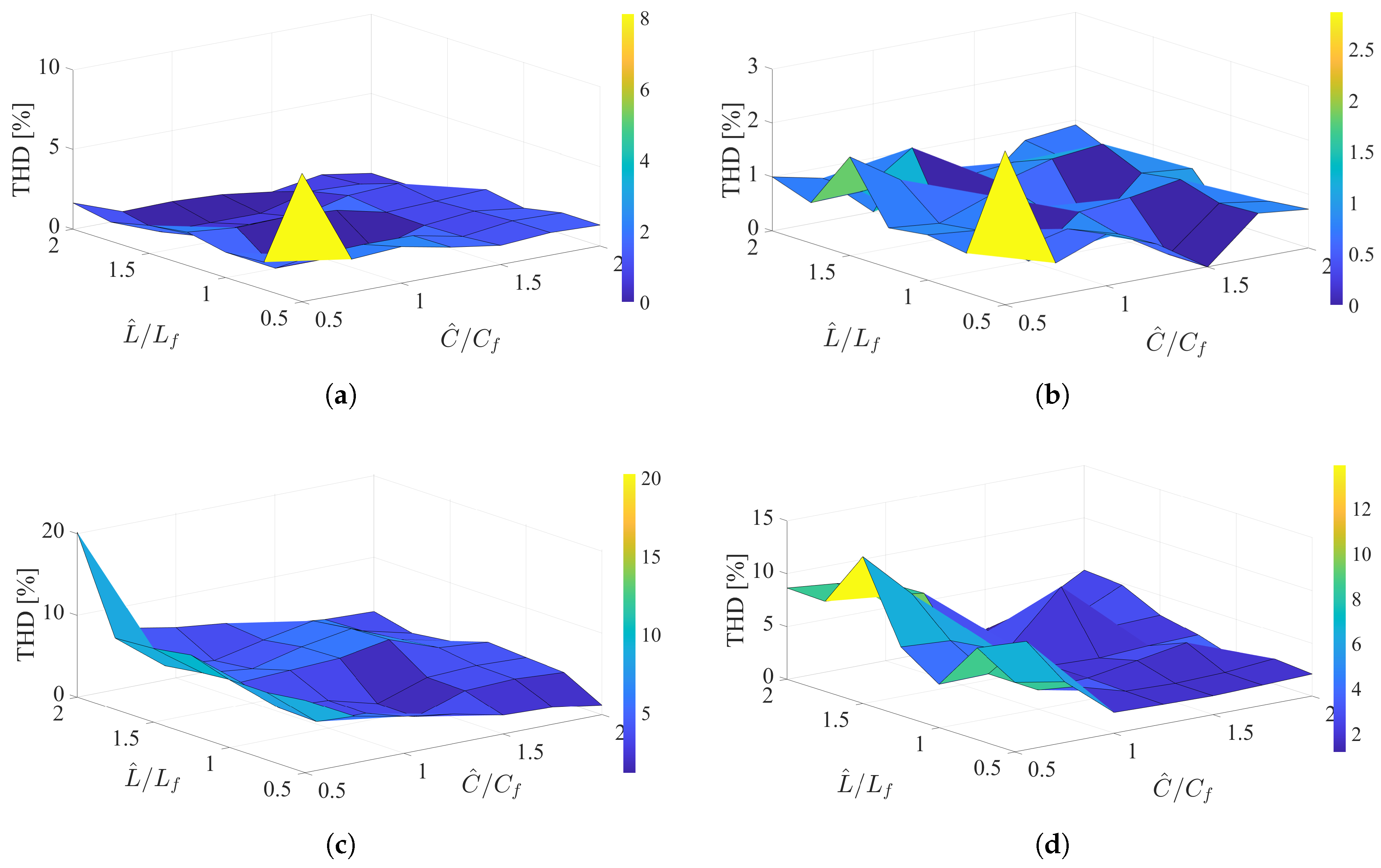
5.4. Steady-State Performance

The steady-state performance will inquire into the relationship between the average switching frequency (as regulated by the switching effort weighting factor ${\chi }_{\mathrm{u}}$) on the output voltage and current THDs. We achieved this by maintaining the weighting factor for current ${\chi }_{\mathrm{i}}$ constant at 3 (gives optimal performance among other heuristically tested values), while ${\chi }_{\mathrm{u}}$ was varied from 0 to 70 in unit steps. The results (comparing conventional MPC and the proposed adaptive MPC) are plotted in Figure 12. The average switching frequency was calculated with $f_{\mathrm{sw}}=\frac{{\sum }_{k=1}^N{u}_{\mathrm{sw}}\left(k\right)}{3N{T}_s}$, where N is the number of samples per second (i.e., 800 for $T_s=25$μs). THDs were obtained with MATLAB/Simulink’s spectrum analyzer. The voltage THD decreased with switching frequency: From 2.5% at 5 kHz to 0.5% at 12 kHz. These results are for nominal filter parameters, and indicate that the proposed method has similar steady-state performance as the conventional MPC.

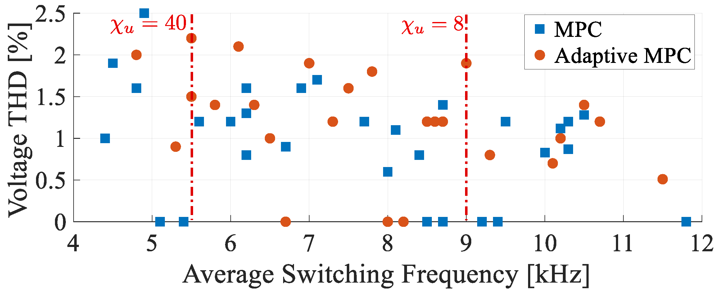
5.5. Overall Performance

Figure 13 illustrates the voltage and current sensitivities to a wide range of parameter variations. These figures show a broader view of the performance of the proposed control algorithm. Adaptive MPC voltage THD has a lower range (3%) than conventional MPC (8%), for almost all ranges of parameter variations of filter inductance and capacitance. In addition, adaptive MPC current THD has a lower range (12%) than conventional MPC (18%).

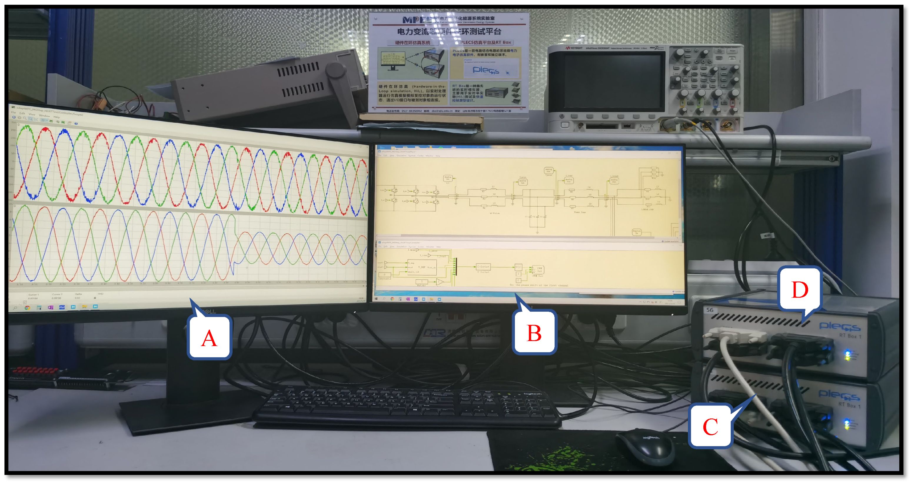
5.6. Real-Time Hardware-in-the-Loop Verification

In this section, the real-time HiL performance will be discussed. We set up the test micrgrid system on a test bench made up of PLECS RT-Box 1 real-time HiL equipment.

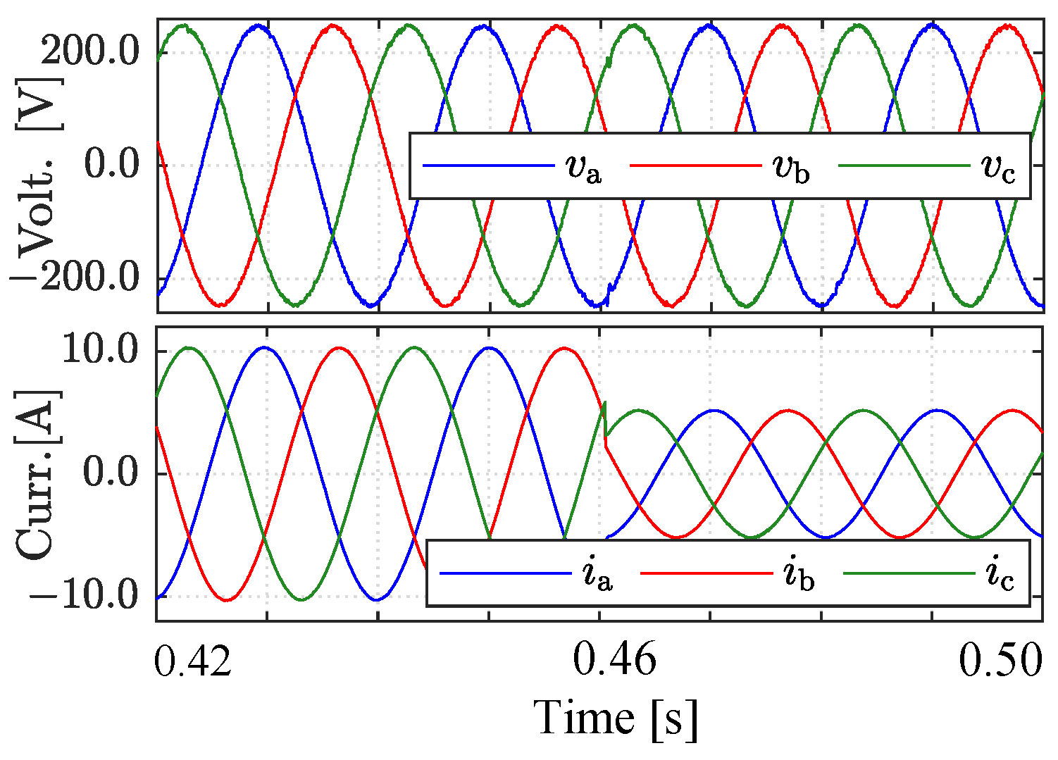
5.6.1. Transient Performance

During the transient, operation rapid and robust transient responses are desired. Figure 14 shows that during the transient period, the proposed control scheme did not lose tracking performance.

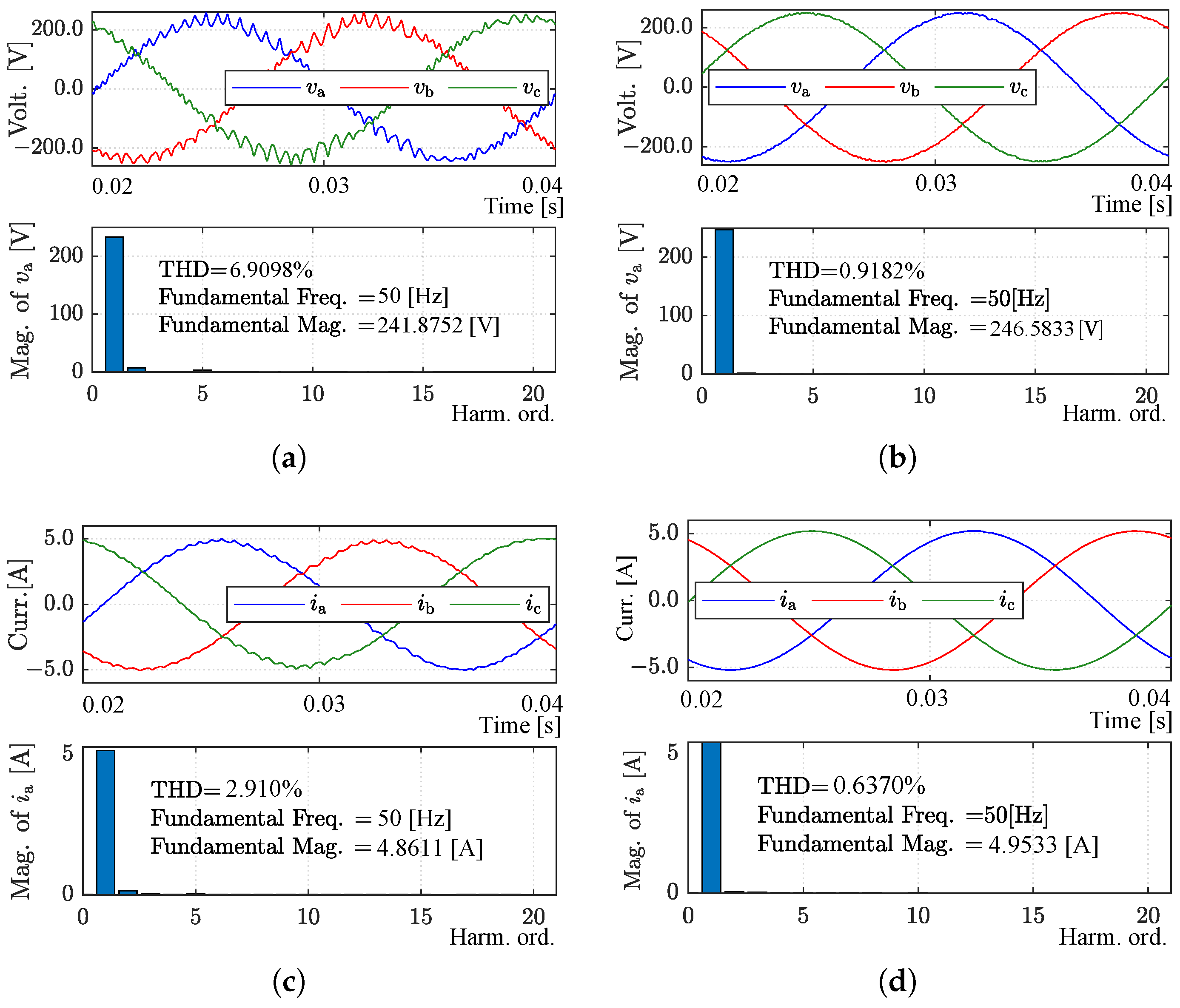
5.6.2. Robustness to Model Parameter Variations

Figure 15 illustrates the conventional MPC and proposed adaptive MPC voltage and current performances for 0.5$L_{\mathrm{f}}$ variation in nominal inductance. The left-hand plots in Figure 15 are for conventional MPC, while the right-hand plots are for adaptive MPC. Comparing the top plots (voltage) shows that the proposed adaptive MPC scheme produces significantly less distortion than the left waveform (63.2% THD reduction). Similarly, the adaptive MPC current waveform on the right is less distorted than the waveform on the left, i.e., 47.6% THD reduction. These results point to the robustness of the proposed control scheme to parameter variations.

6. Conclusions

The performance of predictive-controlled converters deteriorates with parametric mismatches. In this paper, we demonstrated a solution to this problem via the design of a parameter estimator for an operating point, and neuro-fuzzy parameter estimator for wider operating conditions. The latter’s advantages came at the price of a higher estimation computation burden. The simulation and HiL results have demonstrated the effectiveness of the proposed adaptive predictive control of grid-forming converters with an improved power quality and robustness to parameter uncertainties.

In future, we would be interested in examining how other intelligent/data-based methods reduce the computational burden without compromising the performance.

References

1. Matevosyan, J.; Badrzadeh, B.; Prevost, T.; Quitmann, E.; Ramasubramanian, D.; Urdal, H.; Achilles, S.; MacDowell, J.; Huang, S.H.; Vital, V.; et al. Grid-Forming Inverters: Are They the Key for High Renewable Penetration? IEEE Power Energy Mag. 2019, 17, 89–98. [Google Scholar] [CrossRef]
2. Babayomi, O.; Li, Z.; Zhang, Z. Distributed secondary frequency and voltage control of parallel-connected vscs in microgrids: A predictive VSG-based solution. CPSS Trans. Power Electron. Appl. 2020, 5, 342–351. [Google Scholar] [CrossRef]
3. Young, H.A.; Perez, M.A.; Rodriguez, J. Analysis of Finite-Control-Set Model Predictive Current Control With Model Parameter Mismatch in a Three-Phase Inverter. IEEE Trans. Ind. Electron. 2016, 63, 3100–3107. [Google Scholar] [CrossRef]
4. Yang, Y.; Tan, S.; Hui, S.Y.R. Adaptive Reference Model Predictive Control With Improved Performance for Voltage-Source Inverters. IEEE Trans. Control Syst. Technol. 2018, 26, 724–731. [Google Scholar] [CrossRef]
5. Easley, M.; Fard, A.Y.; Fateh, F.; Shadmand, M.B.; Abu-Rub, H. Auto-Tuned Model Parameters in Predictive Control of Power Electronics Converters; IEEE: Baltimore, MD, USA, 2019; pp. 3703–3709. [Google Scholar] [CrossRef]
6. Khalilzadeh, M.; Vaez-Zadeh, S.; Eslahi, M.S. Parameter-Free Predictive Control of IPM Motor Drives with Direct Selection of Optimum Inverter Voltage Vectors. IEEE J. Emerg. Sel. Top. Power Electron. 2021, 9, 327–334. [Google Scholar] [CrossRef]
7. Lin, C.K.; Yu, J.t.; Lai, Y.S.; Yu, H.C. Improved Model-Free Predictive Current Control for Synchronous Reluctance Motor Drives. IEEE Trans. Ind. Electron. 2016, 63, 3942–3953. [Google Scholar] [CrossRef]
8. Carlet, P.G.; Tinazzi, F.; Bolognani, S.; Zigliotto, M. An Effective Model-Free Predictive Current Control for Synchronous Reluctance Motor Drives. IEEE Trans. Ind. Appl. 2019, 55, 3781–3790. [Google Scholar] [CrossRef] [Green Version]
9. Zhang, Y.; Jin, J.; Huang, L. Model-Free Predictive Current Control of PMSM Drives Based on Extended State Observer Using Ultralocal Model. IEEE Trans. Ind. Electron. 2021, 68, 993–1003. [Google Scholar] [CrossRef]
10. Rodriguez, J.; Heydari, R.; Rafiee, Z.; Young, H.A.; Flores-Bahamonde, F.; Shahparasti, M. Model-Free Predictive Current Control of a Voltage Source Inverter. IEEE Access 2020, 8, 211104–211114. [Google Scholar] [CrossRef]
11. Aguilera, R.P.; Lezana, P.; Quevedo, D.E. Finite-Control-Set Model Predictive Control With Improved Steady-State Performance. IEEE Trans. Ind. Inform. 2013, 9, 658–667. [Google Scholar] [CrossRef]
12. Xia, C.; Wang, M.; Song, Z.; Liu, T. Robust Model Predictive Current Control of Three-Phase Voltage Source PWM Rectifier With Online Disturbance Observation. IEEE Trans. Ind. Inform. 2012, 8, 459–471. [Google Scholar] [CrossRef]
13. Martin, C.; Arahal, M.R.; Barrero, F.; Durin, M.J. Five-Phase Induction Motor Rotor Current Observer for Finite Control Set Model Predictive Control of Stator Current. IEEE Trans. Ind. Electron. 2016, 63, 4527–4538. [Google Scholar] [CrossRef]
14. Turker, A.; Buyukkeles, U.; Bakan, A.F. A Robust Predictive Current Controller for PMSM Drives. IEEE Trans. Ind. Electron. 2016, 63, 3906–3914. [Google Scholar] [CrossRef]
15. Chen, Z.; Qiu, J.; Jin, M. Adaptive finite-control-set model predictive current control for IPMSM drives with inductance variation. IET Electr. Power Appl. 2017, 11, 874–884. [Google Scholar] [CrossRef]
16. Bechouche, A.; Abdeslam, D.O.; Seddiki, H.; Rahoui, A. Estimation of Equivalent Inductance and Resistance for Adaptive Control of Three-Phase PWM Rectifiers; IEEE: Florence, Italy, 2016; pp. 1336–1341. [Google Scholar] [CrossRef]
17. Mehreganfar, M.; Saeedinia, M.H.; Davari, S.A.; Garcia, C.; Rodriguez, J. Sensorless Predictive Control of AFE Rectifier With Robust Adaptive Inductance Estimation. IEEE Trans. Ind. Inform. 2019, 15, 3420–3431. [Google Scholar] [CrossRef]
18. Kwak, S.; Moon, U.C.; Park, J.C. Predictive-Control-Based Direct Power Control With an Adaptive Parameter Identification Technique for Improved AFE Performance. IEEE Trans. Power Electron. 2014, 29, 6178–6187. [Google Scholar] [CrossRef]
19. Zhang, Y.; Jiao, J.; Liu, J. Direct Power Control of PWM Rectifiers With Online Inductance Identification Under Unbalanced and Distorted Network Conditions. IEEE Trans. Power Electron. 2019, 34, 12524–12537. [Google Scholar] [CrossRef]
20. Abdelrahem, M.; Hackl, C.M.; Kennel, R. Finite set model predictive control with on-line parameter estimation for active frond-end converters. Electr. Eng. 2018, 100, 1497–1507. [Google Scholar] [CrossRef]
21. Huang, L.; Coulson, J.; Lygeros, J.; Dörfler, F. Data-Enabled Predictive Control for Grid-Connected Power Converters; IEEE: Nice, France, 2019; pp. 8130–8135. [Google Scholar] [CrossRef] [Green Version]
22. Carlet, P.G.; Favato, A.; Bolognani, S.; Dorfler, F. Data-Driven Predictive Current Control for Synchronous Motor Drives; IEEE: Detroit, MI, USA, 2020; pp. 5148–5154. [Google Scholar] [CrossRef]
23. Teiar, H.; Chaoui, H.; Sicard, P. Almost Parameter-Free Sensorless Control of PMSM; IEEE: Yokohama, Japan, 2015; pp. 004667–004671. [Google Scholar] [CrossRef]
24. Akpolat, A.N.; Habibi, M.R.; Dursun, E.; Kuzucuoglu, A.E.; Yang, Y.; Dragicevic, T.; Blaabjerg, F. Sensorless Control of DC Microgrid Based on Artificial Intelligence. IEEE Trans. Energy Convers. 2020. [Google Scholar] [CrossRef]
25. Dragicevic, T.; Vazquez, S.; Wheeler, P. Advanced Control Methods for Power Converters in DG Systems and Microgrids. IEEE Trans. Ind. Electron. 2020. [Google Scholar] [CrossRef]
26. Babayomi, O.; Oluseyi, P.; Keku, G.; Ofodile, N.A. Neuro-Fuzzy Based Fault Detection Identification and Location in a Distribution Network; IEEE: Accra, Ghana, 2017; pp. 164–168. [Google Scholar] [CrossRef]
27. Guo, L.; Hung, J.; Nelms, R. Evaluation of DSP-Based PID and Fuzzy Controllers for DC–DC Converters. IEEE Trans. Ind. Electron. 2009, 56, 2237–2248. [Google Scholar] [CrossRef]
28. Saroha, J.; Singh, M.; Jain, D.K. ANFIS-Based Add-On Controller for Unbalance Voltage Compensation in a Low-Voltage Microgrid. IEEE Trans. Ind. Inform. 2018, 14, 5338–5345. [Google Scholar] [CrossRef]
29. Jabr, H.M.; Lu, D.; Kar, N.C. Design and Implementation of Neuro-Fuzzy Vector Control for Wind-Driven Doubly-Fed Induction Generator. IEEE Trans. Sustain. Energy 2011, 2, 404–413. [Google Scholar] [CrossRef]
30. Hou, S.; Chu, Y.; Fei, J. Robust Intelligent Control for a Class of Power-electronic Converters Using Neuro-Fuzzy Learning Mechanism. IEEE Trans. Power Electron. 2021. [Google Scholar] [CrossRef]
31. Dragicevic, T. Model Predictive Control of Power Converters for Robust and Fast Operation of AC Microgrids. IEEE Trans. Power Electron. 2018, 33, 6304–6317. [Google Scholar] [CrossRef]
32. Wang, J.S.; Lee, C. Self-adaptive neuro-fuzzy inference systems for classification applications. IEEE Trans. Fuzzy Syst. 2002, 10, 790–802. [Google Scholar] [CrossRef]
33. Er, M.J.; Mandal, S. A Survey of Adaptive Fuzzy Controllers: Nonlinearities and Classifications. IEEE Trans. Fuzzy Syst. 2016, 24, 1095–1107. [Google Scholar] [CrossRef]
Figure 1. A microgrid system with converter-interfaced distributed generation and common loads.
Sustainability 13 07038 g001
Figure 2. Block diagram of the proposed adaptive model predictive control scheme.
Sustainability 13 07038 g002
Figure 3. The adaptive estimator of inductance and capacitance variations. m 1 = 1 / ( L f i f _ amp ) , m 2 = 10 e 3 , where L f is the filter inductance nominal value, and i f _ amp is the filter inductance current amplitude. Also, n 1 = 1 / ( C f v f _ amp ) and n 2 = 0 , where where C f is the filter capacitance nominal value, and v f _ amp is the filter capacitance voltage amplitude.
Sustainability 13 07038 g003
Figure 4. Structure of a four-layer neuro-fuzzy system.
Sustainability 13 07038 g004
Figure 5. Proposed adaptive predictive control for VSCs with neuro-fuzzy parameter estimation, where L ^ = L f + Δ L , C ^ = C f + Δ C , and v ϵ , i ϵ are defined by (A4) and (A13) respectively.
Sustainability 13 07038 g005
Figure 6. Workflow for implementing the proposed neuro-fuzzy parameter estimation.
Sustainability 13 07038 g006
Figure 7. Input membership functions: (a) Before training and (b) after training with offline data.
Sustainability 13 07038 g007
Figure 8. Real-time HiL system: A—signal monitor, B—PLECS user interface monitor, C—real-time controller, and D—plant emulator.
Sustainability 13 07038 g008
Figure 9. Simulation results: Estimated and actual capacitance variations—Top: 0.5 C f variation, bottom: 0.3 C f variation.
Sustainability 13 07038 g009
Figure 10. Simulation results: Estimated and actual inductance variations for 0.5 L f variation, bottom: 0.4 L f variation.
Sustainability 13 07038 g010
Figure 11. Simulation results: Performance of the neuro-fuzzy adaptive controller with 0.5 L f variation in nominal induactance.
Sustainability 13 07038 g011
Figure 12. Conventional MPC voltage THD versus average switching frequency for current term weighting factor χ i = 3 , while switching weighting factor χ u is varied.
Sustainability 13 07038 g012
Figure 13. Sensitivity of output voltage to model mismatches. (a) Voltage—conventional MPC rseponse, (b) voltage—adaptive MPC response, (c) current—conventional MPC response, and (d) current—adaptive MPC response.
Sustainability 13 07038 g013
Figure 14. HIL Results: The proposed adaptive MPC response to a step change in power.
Sustainability 13 07038 g014
Figure 15. HiL Results: MPC and the proposed adaptive MPC voltage and current performances for 0.5 L f variation in nominal inductance. (a) Conventional MPC voltage and spectrum. (b) Proposed adaptive MPC voltage and spectrum. (c) Conventional MPC current and spectrum. (d) Proposed adaptive MPC current and spectrum.
Sustainability 13 07038 g015