Using Quantile Regression to Analyze the Relationship between Socioeconomic Indicators and Carbon Dioxide Emissions in G20 Countries

Abstract

Numerous studies addressed the impacts of social development and economic growth on the environment. This paper presents a study about the inclusive impact of social and economic factors on the environment by analyzing the association between carbon dioxide (CO₂) emissions and two socioeconomic indicators, namely, Human Development Index (HDI) and Legatum Prosperity Index (LPI), under the Environmental Kuznets Curve (EKC) framework. To this end, we developed a two-stage methodology. At first, a multivariate model was constructed that accurately explains CO₂ emissions by selecting the appropriate set of control variables based on model quality statistics. The control variables include GDP per capita, urbanization, fossil fuel consumption, and trade openness. Then, quantile regression was used to empirically analyze the inclusive relationship between CO₂ emissions and the socioeconomic indicators, which revealed many interesting results. First, decreasing CO₂ emissions was coupled with inclusive socioeconomic development. Both LPI and HDI had a negative marginal relationship with CO₂ emissions at quantiles from 0.2 to 1. Second, the EKC hypothesis was valid for G20 countries during the study period with an inflection point around quantile 0.15. Third, the fossil fuel consumption had a significant positive relation with CO₂ emissions, whereas urbanization and trade openness had a negative relation during the study period. Finally, this study empirically indicates that effective policies and policy coordination on broad social, living, and economic dimensions can lead to reductions in CO₂ emissions while preserving inclusive growth.

1. Introduction

Climate change has become a global challenge to all earth inhabitants [1,2]. In 2015, the United Nations Framework Convention on Climate Change (UNFCCC) responded to the climate change risks by adopting the Paris Climate Change Agreement [3]. This agreement aims to “limit global warming to well below 2 degrees Celsius, preferably to 1.5 degrees Celsius, compared to pre-industrial levels”. Many studies have proven that human activities such as burning fossil fuels are the main causes of increasing heat temperatures, which contribute to global warming and escalate the speed of changes in the climate system [4,5,6].

Understanding the causes of global CO₂ emissions has attracted the attention of researchers and policy makers alike. This study addresses the inclusive relationship between socioeconomic indicators and CO₂ emissions. The aim is to understand the collective impact of multiple social and economic factors on the environment. A well-defined socioeconomic indicator is the Legatum Prosperity Index (LPI), which provides a methodology to measure prosperity [7]. LPI defines prosperity to cover three domains: inclusive societies, open economies, and empowered people. These three domains are divided into 16 pillars, which are further subdivided into 66 elements. Crafted mathematical formulas are used to compute score values for each of these elements, which are then aggregated to constitute LPI (In this paper, we excluded the emissions element from LPI score to eliminate any bias to the dependent variable which is CO₂ emissions). The Human Development Index (HDI) is another well-established socioeconomic indicator [8]. HDI is computed as the geometric mean of three indices: Gross National Income (GNI), education index, and life expectancy index. These indices represent standard of living, knowledge, and long and healthy life, respectively.

A recent study addressed the need to evaluate the existing integrated assessment models for climate change and come up with more realistic mitigation policies [9]. Another study highlighted the importance of the trade-off between socioeconomic factors and sustainable development goals when it comes to climate change mitigation [10]. According to the World Bank [11], CO₂ emissions produced from burning fossil fuels and industrial activities are responsible for almost 60% of GHG emissions. In fact, the data show that from 1970 to 2010, the CO₂ emissions from fossil fuel combustion and industrial processes accounts for about 78% of the increase in total GHG emissions [5,6,12].

The theoretical underpinnings suggest that CO₂ emissions pose great risks to the prosperity of humans on this planet [13]. Scholars believe that fundamental human needs such as health, food security, and economic development could be hindered as CO₂ emissions rise. They recommend that countries around the world take actions to reduce their CO₂ emissions by engaging in activities that are friendly to the environment. As stated, there has not been a study devoted to measuring the relationship between socioeconomic indicators and CO₂ emission for G20 countries. In this regard, there is a need to conduct a study that takes into account multiple social and economic variables and their inclusive relationship to CO₂ emissions.

Over the past three decades, understanding the drivers of CO₂ emissions has drawn considerable attention from researchers in different fields. Previous studies have focused on the relationship between income and environmental degradation. The economic growth, measured by GDP, has been studied extensively as one of the main explanatory variables that influence CO₂ emissions [14,15]. In a study conducted in Azerbaijan, scholars have found a positive relationship between economic growth and CO₂ emissions. The study concluded that countries should take measures to enhance the environment and reduce their carbon emissions. The scholars suggest enacting policies toward increasing energy efficiency, lowering pollution from trade activities, and promoting social awareness programs [5].

This study addressed the widely studied nonlinear relationship between economic growth and environmental degradation, known as Environmental Kuznets Curve (EKC), based on the theory of Kuznets, who suggested an inverted U-shaped relation between income distribution and economic development [16]. Many studies investigated the EKC hypothesis for CO₂ emissions and discovered that economic growth caused environmental degradation in early stages and then, at some point, the trend peaked and reversed the direction for the better of the environment [17,18]. Many other studies had focused on the relationship between income and environmental degradation. Grossman and Krueger [19] showed that economic growth deteriorates the environment at an initial phase followed by an improvement phase using panel data from 39 developed and developing countries. Another work compared the short-run and long-run income elasticities to examine the EKC hypothesis in 43 developing countries and concluded that it is valid in 15 countries [20]. On the other hand, there is no common consensus about the validity of the EKC hypothesis. An empirical evaluation using an ARDL model showed a U-shaped relation between CO₂ emissions and income in Greenland [21]. Another work showed a positive relation between pollution and economic growth [22].

Other studies examined different variables; nonetheless, they apply similar concepts or tools. Wang et al. [23] conducted a study about the influence of trade openness on CO₂ emissions and found a positive relation, since trade openness encourages more production, which increases pollution. In another case study [24], the authors concluded that trade openness facilitates clean production using advanced technology, which improves the environment. The influence of population density on CO₂ emissions was studied by Chen et al. [25], and they discovered a positive relation for developing countries and a negative relation for developed countries. Lv and Li [26] examined the effect of financial development on CO₂ emission. They found that there was a positive correlation between CO₂ emissions and financial development. However, their results also indicate that there was a significantly negative spatial correlation between CO₂ emissions among neighboring countries. Moreover, the data show that there was a significant negative spillover effect of financial development on CO₂ emissions. These findings suggest that a country with high financial development could improve a neighboring country’s environmental performance. The work by Angel et al. [27] built on the assumption that urban growth is associated with decreasing GHG emission and studied urban expansion and densification in 200 cities around the world during the period 1990 to 2014. They concluded that a trade-off between densifying and expanding cities should be targeted based on population increase and economic growth. On contrary, other studies support the assumption that urbanization increases carbon emissions [28,29].

In this paper, we focus the attention on the influence of inclusive socioeconomic development on CO₂ emissions in the G20 countries. These countries include wide variations in economic and social dimensions, which together account for around 90% of world GDP, 80% of global trade, 60% of world population, and about half of the global land area [30]. Unlike many previous studies that focused solely on economic growth, we adopt two inclusive indicators that cover pivotal economic and social well-being: LPI and HDI. To study their association with CO₂ emissions, we developed two multivariate models that adequately explain CO₂ emissions using relevant control variables. To this end, we considered GDP per capita, fossil fuel consumption, urbanization, and trade openness, whose associations with CO₂ have been well-studied [4,13,24,31,32]. Then, two models were constructed with LPI and HDI to analyze their relationship with CO₂ emissions using quantile regression.

Our study contributes to the literature as follows: (i) This is the first study that investigates the relationship between inclusive socioeconomic indicators and CO₂ emissions. (ii) We modelled the per capita CO₂ emissions using two socioeconomic indicators and four well-studied control variables, i.e., per capita GDP, fossil fuel consumption, urbanization, and trade openness. (iii) We empirically tested the EKC hypothesis. (iv) We applied the most recent data for all G20 countries, which widely represent the world and include a period after the Paris climate change agreement [3]. The remainder of this paper is organized as follows. Section 2 presents the materials and methods, Section 3 provides results and discussion, and Section 4 concludes the study with policy implications.

2. Materials and Methods

This paper utilized an empirical approach to analyze data from 2000 to 2019 to understand the overall relationship between CO₂ emissions and socioeconomic indicators represented by LPI and HDI. Figure 1 shows the main steps of our study. At first, a set of well-studied drivers of CO₂ emissions were considered as model control variables. To this end, data for gross domestic product (GDP), fossil fuel consumption (FC), urbanization (URB), trade openness (TR), and population density (PD) were utilized. The outcome of the variable selection method is a subset of the original set of variables, which are selected based on their goodness of explanation and statistical significance. Then, two multivariate models were constructed with LPI and HDI to analyze their association with CO₂ emissions using quantile regression.

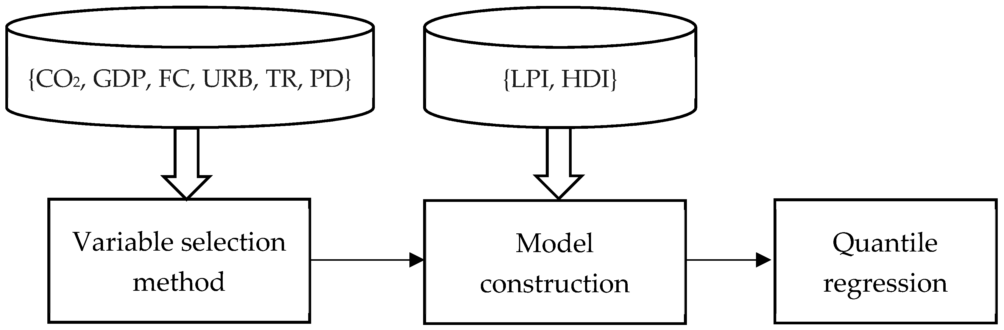
2.1. Data and Variable Selection

This study used the annual data for G20 countries for eight variables, as shown in

Table 1. Data description of variables.

Variable	Description	Unit	Years	Data Source
CO2	CO2 emissions per capita including sources from fossil fuel use and industrial processes	ton CO2/capita	2000–2019	[33]
LPI	Legatum Prosperity Index	Percentage	2007–2019	[7]
HDI	Human Development Index	Percentage	2000–2019	[8]
GDP	GDP per capita expressed in current USD converted by PPP conversion factor	USD/capita	2000–2019	[34]
FC	Fossil fuel consumption per capita	kWh/capita	2000–2019	[35]
TR	The sum of exports and imports of goods and services measured as a share of GDP	Percentage of GDP	2000–2019	[34]
URB	People living in urban areas (% of total population)	Percentage	2000–2019	[34]
PD	The number of persons per square km	Persons/km2	2000–2019	[34]

. These variables include CO₂, LPI, and HDI, which are the main focus of this study. The other variables (GDP, FC, TR, URB, and PD) were considered for selecting control variables in our model. Due to the complexity and nonlinearity of CO₂ emissions, a model that comprehend an adequate set of control variables is needed to study the relationship with the indicators LPI and HDI. That is, a set of N explanatory variables X_i are related to CO₂ as follows:

$$lnC{O}_{2t}={\alpha }_0+{\displaystyle \sum }_{n=1}^N{\alpha }_{n}ln{X}_{nt}$$

(1)

where ln is the natural logarithm; CO_2t is the per capita CO₂ emissions at year t; X_n is the n-th explanatory variable; N is the number of explanatory variables; α₀ … α_N are the model parameters. The aim is to select a subset of control variables that best explains the dependent variable using quantile regression (explained in Section 2.3). For each possible subset of the N explanatory variables (there are 2^N − 1 possible subsets), the model parameters are computed at 50% quantile along with the adjusted R-squared, mean absolute error (MAE), and statistical significance. These three statistical metrics reflect the model quality and are used for selecting the control variables in the models for analyzing the relationship between CO₂ emissions and the socioeconomic indicators.

2.2. Empirical Model

To study the inclusive relationship between the socioeconomic indicators and CO₂ emissions, two empirical models were considered for LPI and HDI as follows:

$$\mathrm{Model}1:lnC{O}_{2it}={\beta }_0+{\beta }_{1}lnLP{I}_{it}+{\beta }_{2}lnGD{P}_{it}+{\beta }_3{(lnGD{P}_{it})}^2+{{\displaystyle \sum }}_{j=1}^r{\gamma }_j{X}_{itj}$$

(2)

$$\mathrm{Model}2:lnC{O}_{2it}={\delta }_0+{\delta }_{1}lnHD{I}_{it}+{\delta }_{2}lnGD{P}_{it}+{\delta }_3{\left(lnGD{P}_{it}\right)}^2+{{\displaystyle \sum }}_{j=1}^r{\gamma }_j{X}_{itj}$$

(3)

where ln is the natural logarithm, CO_2it is per capita CO₂ emissions with I ∈ {G20 countries} and t ∈ [2000:2019], LPI and HDI are socioeconomic indicators, GDP is per capita GDP, and $\left\{X_j\right\}\subseteq \left\{FC,URB,TR,PD\right\}$ are control variables selected according to Equation (1). All G20 countries were covered in this study with an exception of the EU (which consisted of 28 countries during the study period, out of which four countries were included in the study, namely, France, Germany, Italy, and the UK). The parameters β₀, …, β₃, δ₀, …, δ₃ are the elasticity estimates of the explanatory variables. The quadratic term of the per capita GDP was introduced in the models to empirically test the EKC hypothesis. When β₂ is positive and β₃ is negative, this means an inverted U-shape pattern is detected [36]. Meanwhile, if β₂ is negative and β₃ is positive, this means a U-shape pattern is detected. When both β₂ and β₃ are positive (negative), a monotonically increasing (decreasing) pattern holds. For the coefficients of LPI and HDI (β₁, δ₁), positive (negative) values mean more (less) CO₂ emissions.

2.3. Quantile Regression

Quantile regression (QR), introduced by Koenker and Bassett [37], is a common approach in econometrics for parameter estimation and analysis of models. Compared to the ordinary least squares (OLS) method that estimates the conditional mean of the dependent variable, QR is median-based and aims at estimating quantiles of the dependent variable. Suppose y and x are dependent and independent variables, respectively. Assuming linearity in the conditional relation y|x leads to the following:

$${\mathrm{y}}_q=x_i^{\prime }{\beta }_q$$

(4)

where β_q is the coefficient of the q quantile, $q\in \left[0,1\right]$. β_q can be estimated by minimizing the following sum of absolute differences objective function:

$$\underset{{\beta }_q}{\min }{{\displaystyle \sum }}_{i\in \left\{y_{i }\ge x_i^{\prime }{\beta }_q\right\}}q\left|y_i-x_i^{\prime }{\beta }_q\right|+{{\displaystyle \sum }}_{i\in \left\{y_i<x_i^{\prime }{\beta }_q\right\}}\left(1-q\right)\left|y_i-x_i^{\prime }{\beta }_q\right|.$$

(5)

The parameters in Equation (5) can be evaluated using linear programming [38]. By varying q gradually from 0 to 1 and solving for β_q, a plot is obtained for each explanatory variable that explains its relation with the dependent variable. The QR estimation is more robust to outliers and wide variations in data than the OLS estimation. More importantly, when the distribution of the dependent variable does not follow the normal distribution, which is the case for most environmental and economic data, OLS estimation becomes unreliable whereas QR estimation can detect the heterogeneous relations with the dependent variable [39].

3. Results and Discussion

3.1. Data Statistics

The statistical descriptors of the variables in this study are shown in

Table 2. Data statistics of the variables.

Variables	CO2	LPI	HDI	GDP	URB	FC	TR	PD
Mean	8.77	66.13	80.4	22209	73.1	35421	52.1	139.6
Std. dev.	5.49	10.52	10.9	17673	15.3	23887	17.6	147.5
Median	8.19	60.2	83.7	15698	78.9	28709	52.1	93.3
Skewness	0.51	0.11	−0.68	0.49	−1.43	0.64	0.31	1.12
Kurtosis	−0.83	−1.67	−0.53	−1.05	1.35	−0.64	−0.17	0.24
Jarque–Bera	248 ***	225 ***	227 ***	274 ***	173 ***	236 ***	165 ***	200 ***
Observations	380	247	380	380	380	380	380	380
Units	ton CO2/capita	Percentage	Percentage	USD/capita	Percentage	kWh/capita	Percentage of GDP	Persons/km2

Note: *** Significance at a level below 1%.

. The skewness and kurtosis descriptors were computed based on third-order and fourth-order central moments, respectively. The skewness reflects the asymmetry of the distribution, whereas kurtosis describes its steepness. The Jarque-Bera test [40] scores indicate that the null hypothesis is rejected for all variables, which means they do not follow the normal distribution. Therefore, the OLS is not accurate for parameter estimation when modeling these variables.

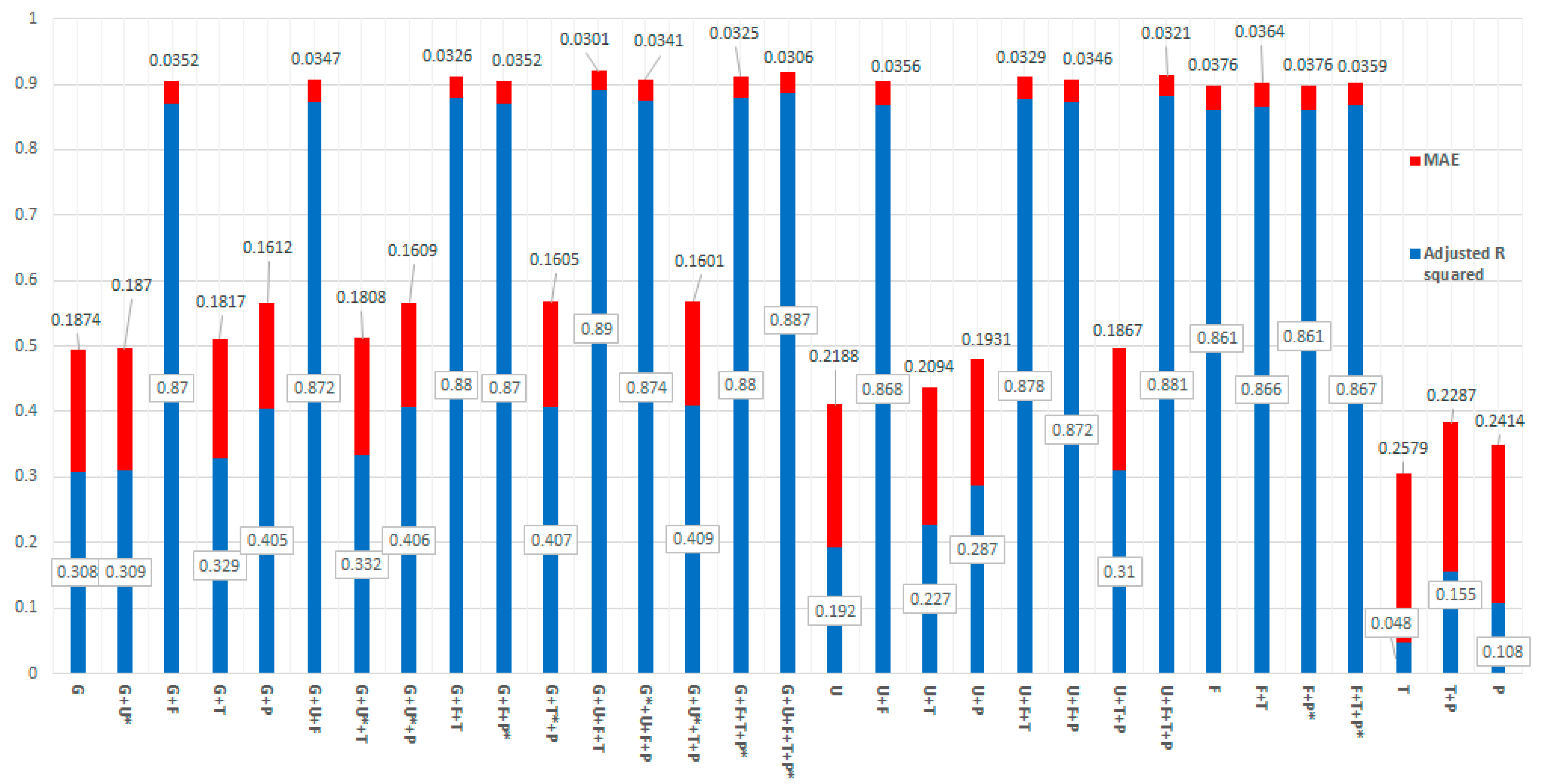
3.2. Control Variables Selection

In this study, we empirically selected the control variables of the regression models as described in Section 2.1. The aim was to select a subset from a group of explanatory variables (GDP, URB, FC, TR, and PD) that is statistically significant and yields the highest adjusted R-squared value and lowest MAE. To this end, regression parameters of Equation (1) were computed for 2⁵ − 1 = 31 subsets of variables, as depicted in Figure 2. From the figure, GDP, URB, FC, and TR returned the highest adjuster R-squared value of 0.89 and lowest MAE of 0.0301 with all variables were statistically significant. Therefore, they were considered as control variables in models 1 and 2 of Equations (2) and (3).

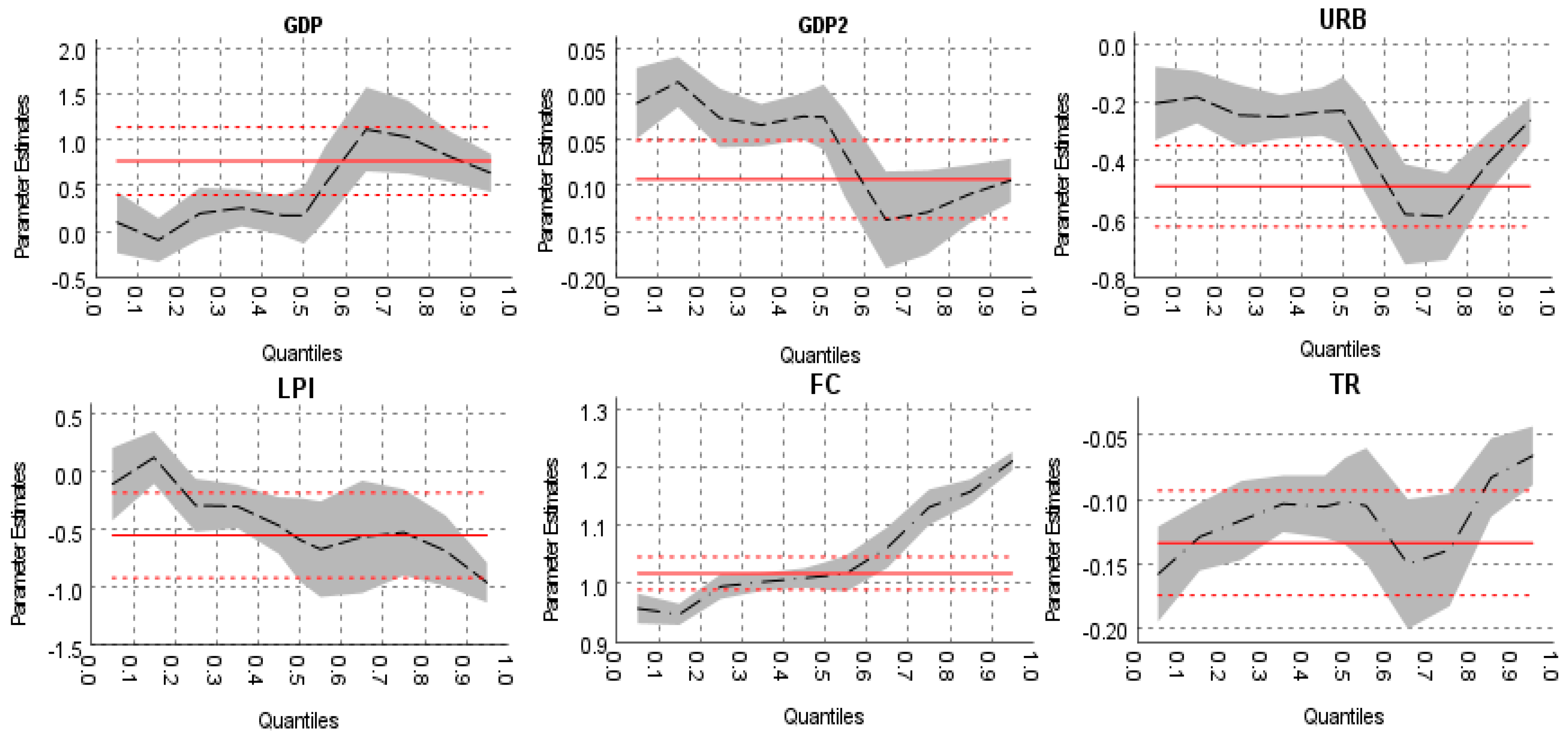
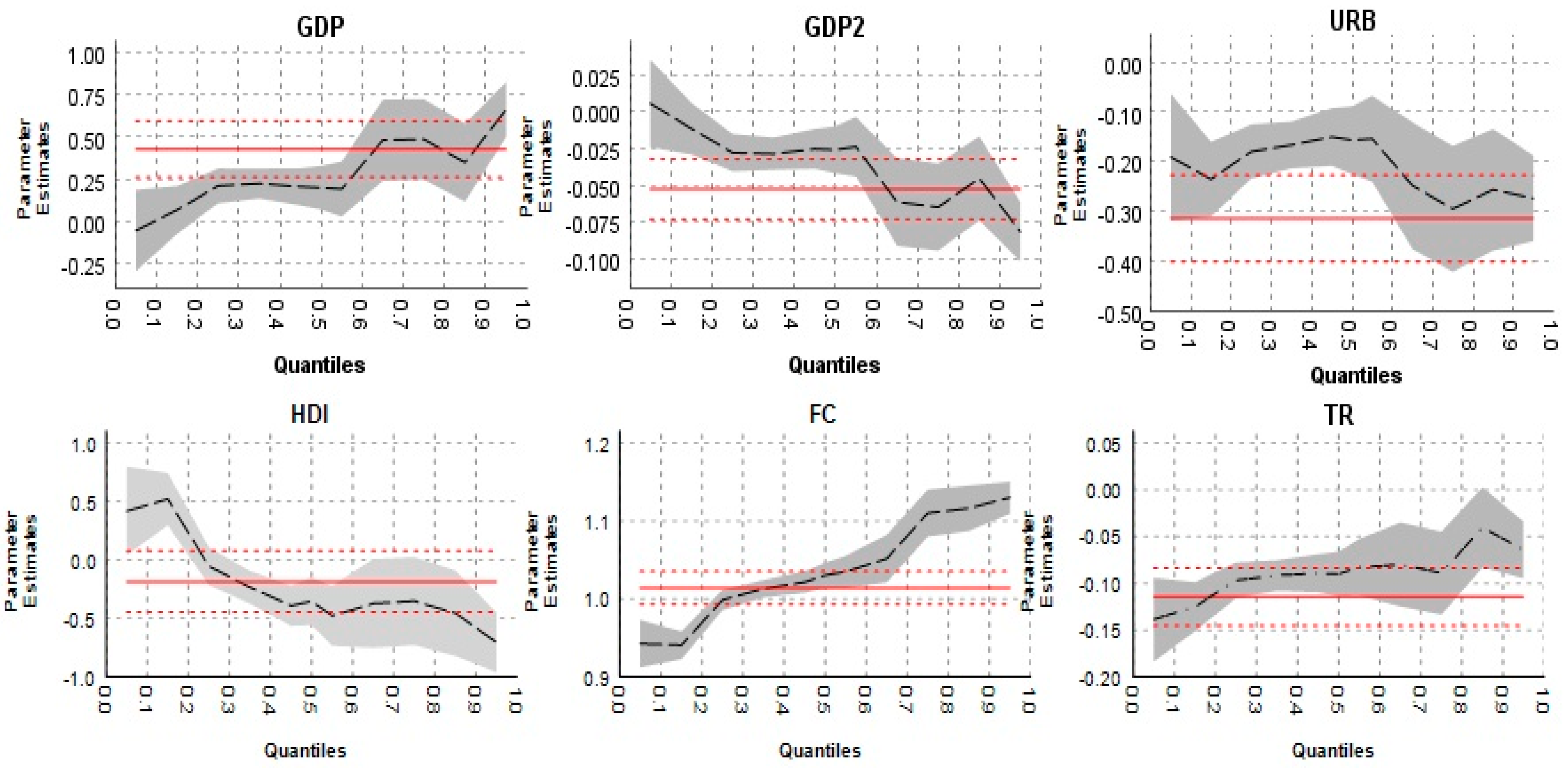
3.3. Empirical Analysis

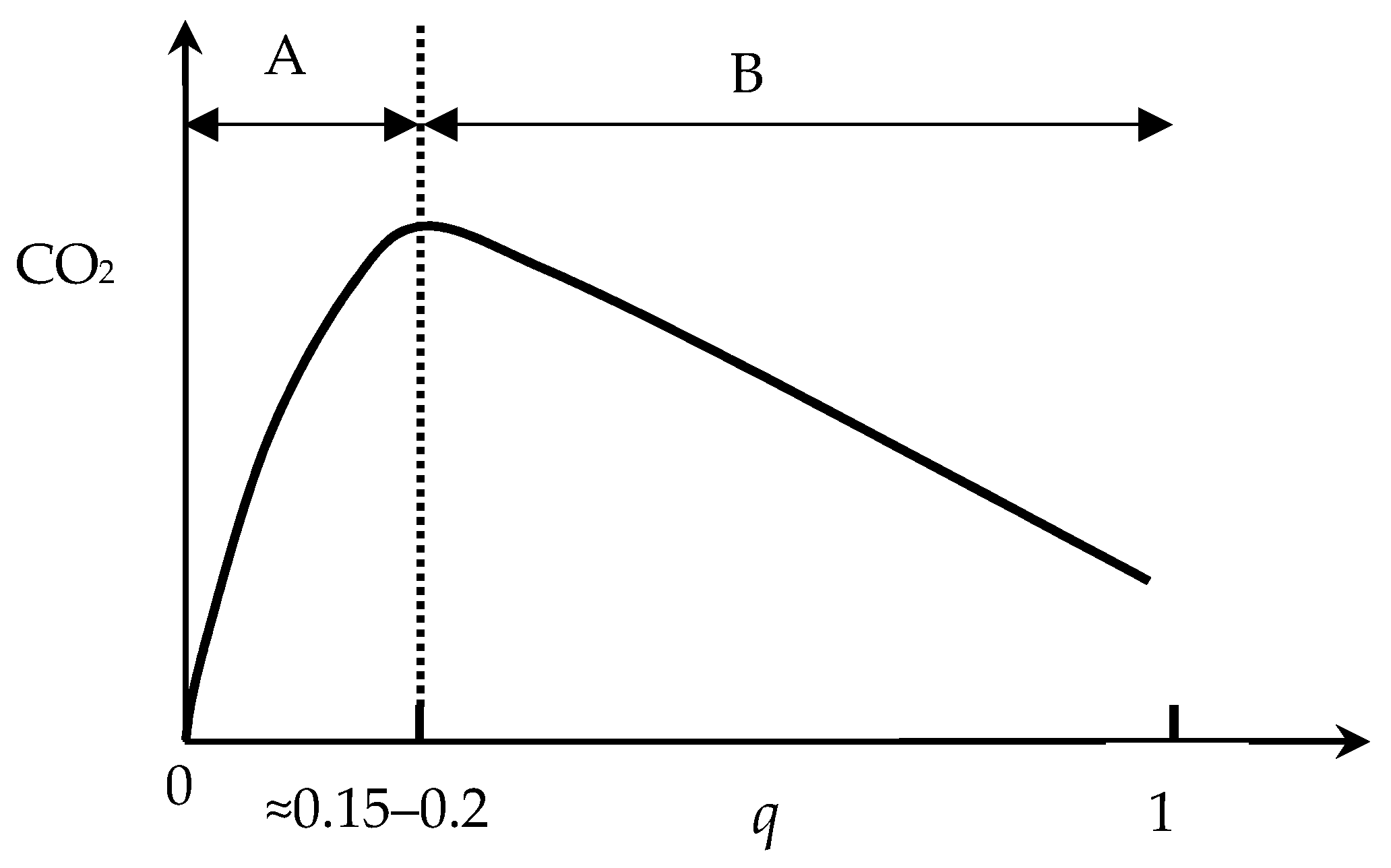
The empirical analysis was carried out by estimating the model parameters of the explanatory variables using quantile regression and then interpreting their relations with the CO₂ emissions. In this study, LPI and HDI were employed to represent socioeconomic indicators. Based on the selected control variables in Section 3.2, Equations (3) and (4) can be rewritten as follows:

$$\mathrm{Model}1:lnC{O}_{2it}={\beta }_0+{\beta }_{1}lnLP{I}_{it}+{\beta }_{2}lnGD{P}_{it}+{\beta }_3{(lnGD{P}_{it})}^2+{\beta }_{4}lnUR{B}_{it}+{\beta }_{5}lnF{C}_{it}+{\beta }_{6}lnT{R}_{it}$$

(6)

$$\mathrm{Model}2:lnC{O}_{2it}={\delta }_0+{\delta }_{1}lnHD{I}_{it}+{\delta }_{2}lnGD{P}_{it}+{\delta }_3{(lnGD{P}_{it})}^2+{\delta }_{4}lnUR{B}_{it}+{\delta }_{5}lnF{C}_{it}+{\delta }_{6}lnT{R}_{it}.$$

(7)

Figure 3 and Figure 4 show the quantile regression plots of the per capita CO₂ emissions (horizontal axes) versus each explanatory variable (vertical axes) for LPI and HDI, respectively. In both figures, q was changed gradually from 0.05 to 0.95 with 0.05 steps. The vertical axes in the plots depict estimation of the parameters β₁, …, β₆ in model 1 and δ₁, …, δ₆ in model 2. For comparison purposes, the red horizontal line in each plot represents the estimated coefficient obtained by the OLS and its corresponding 95% confidence interval indicated by the dotted lines. The curve represents the estimated coefficient using QR, and the shaded area shows the corresponding 95% confidence interval.

Table 3. Quantile regression results at different quantiles for the relations between model 1 variables of Equation (6) in G20 countries from 2007 to 2019.

Variable	q0.05	q0.25	q0.50	q0.75	q0.95
(Intercept)	−3.066 ***	−3.320 ***	−3.367 ***	−4.481 ***	−4.866 ***
	(0.000)	(0.000)	(0.000)	(0.000)	(0.000)
GDP	0.102	0.199 *	0.177 ***	1.033 ***	0.640 ***
	(0.153)	(0.0.064)	(0.002)	(0.000)	(0.000)
GDP2	−0.010	−0.026 **	−0.025 ***	−0.129 ***	−0.094 ***
	(0.220)	(0.0049)	(0.001)	(0.000)	(0.000)
URB	−0.203 ***	−0.244 ***	−0.228 ***	−0.593 ***	−0.261 ***
	(0.002)	(0.000)	(0.000)	(0.000)	(0.000)
LPI	−0.102 *	−0.285 ***	−0.583 ***	−0.520 ***	−0.955 ***
	(0.040)	(0.015)	(0.002)	(0.000)	(0.000)
FC	0.957 ***	0.995 ***	1.013 ***	1.131 ***	1.211 ***
	(0.000)	(0.000)	(0.000)	(0.000)	(0.000)
TR	−0.158 ***	−0.116 ***	−0.101 ***	−0.139 ***	−0.066 ***
	(0.000)	(0.000)	(0.000)	(0.000)	(0.000)
Observations	247	247	247	247	247

Note: The numbers in parentheses are standard errors. ***, **, and * stand for the significance level of 1%, 5%, and 10%, respectively.

and

Table 4. Quantile regression results at different quantiles for the relations between model 2 variables of Equation (7) in G20 countries from 2000 to 2019.

Variable	q0.05	q0.25	q0.50	q0.75	q0.95
(Intercept)	−3.466 ***	−3.390 ***	−2.987 ***	−3.566 ***	−3.462 ***
	(0.000)	(0.000)	(0.000)	(0.000)	(0.000)
GDP	−0.056	0.209 ***	0.197 ***	0.485 ***	0.662 ***
	(0.247)	(0.000)	(0.003)	(0.000)	(0.000)
GDP2	0.006	−0.028 ***	−0.026 ***	−0.065 ***	−0.082 ***
	(0.314)	(0.000)	(0.001)	(0.000)	(0.000)
URB	−0.191 ***	−0.180 ***	−0.157 ***	−0.295 ***	−0.274 ***
	(0.003)	(0.000)	(0.000)	(0.000)	(0.000)
HDI	0.420 **	−0.054 ***	−0.353 ***	−0.351 ***	−0.706 ***
	(0.030)	(0.003)	(0.001)	(0.001)	(0.000)
FC	0.942 ***	0.999 ***	1.030 ***	1.110 ***	1.130 ***
	(0.000)	(0.000)	(0.000)	(0.000)	(0.000)
TR	−0.139 ***	−0.097 ***	−0.090 ***	−0.089 ***	−0.064 ***
	(0.000)	(0.000)	(0.000)	(0.000)	(0.000)
Observations	380	380	380	380	380

Note: The numbers in parentheses are standard errors. *** and ** stand for the significance level of 1% and 5% respectively.

show the quantile regression results for the explanatory variables at different q values for LPI and HDI, respectively. Due to data availability, LPI was analyzed for the period from 2007 to 2019, whereas HDI was analyzed from 2000 to 2019. In the following, we analyze the influence of the explanatory variables on CO₂ emissions in both cases of LPI and HDI. For the intercept coefficients, their values were included in Table 3 and Table 4, but their plots were not included due to space limitations. Intercept coefficients are useful for prediction applications and not important for analyzing the marginal effects of the explanatory variables.

3.4. Discussion

This subsection provides discussion about the results of this paper and comparison with similar works in the literature. For both LPI and HDI, there was a negative marginal relationship with CO₂ emissions at quantiles larger than 0.2, with this relation becoming more significant as the quantile increases. This means that improved socioeconomic development was related to reductions in the CO₂ emissions in G20 countries except those below the 0.2 quantile. For the per capita GDP, the effect on CO₂ emission was positive for all quantiles. To empirically validate the EKC hypothesis, we analyzed the coefficient of the squared per capita GDP, which was negative for quantiles larger than 0.15. This indicates that a persistent increase in the per capita GDP can lead to reductions in the per capita CO₂ emissions. We conclude that the EKC hypothesis was applicable to the G20 during the period of study. This conclusion is consistent with the findings of [18,19,20,41] and against those of [21,22]. An interesting finding is the link between EKC curve, LPI, and HDI turning points in relation with CO₂ emissions. As illustrated in Figure 5, at low quantiles (interval A), all GDP, squared GDP, LPI, and HDI had positive relations with CO₂ emissions. Whereas in interval B, squared GDP, LPI, and HDI had negative relations. This evidence supports the assumption that at early stages of development, an improved socioeconomic development is associated with an increase in CO₂ emissions. However, as economic and social development matures, increasing GDP is associated with reductions in CO₂ emissions.

For the control variables, the empirical results in this paper show that increasing urbanization in G20 countries is associated with reductions in CO₂ emissions, which agrees with the results on G20 countries data by Chen et al. [25] and does not agree with the finding using data of USA [31] and Bangladesh [42]. We hypothesize that different patterns of urbanization depending on social and economic circumstances have distinct impacts on the environment. In addition, there is consensus in the research community that increased fossil fuel consumption is coupled with increased CO₂ emissions [31,43], which this study confirms as well. Finally, this study revealed that increased trade openness is associated with reduction in CO₂ emissions, which agrees with the work by Chen et al. [25] on data from G20 countries and by Dogan and Turkekul [31] on USA, and disagrees with another work on 64 countries [44]. Our interpretation to this variation is that trade openness impact on CO₂ emissions is related to the nature of goods and services being imported and exported and their impact on the environment. Economies that import goods and services that release high CO₂ emissions during production can reduce their emissions quota compared with producing them locally. In addition, opening trade between countries allows market access and stimulates increased production and more waste and pollution from the burning of fossil fuels.

4. Main Conclusions and Policy Implications

This study investigated the inclusive relationship between socioeconomic indicators and CO₂ emissions in G20 countries using two socioeconomic indicators: LPI for the period 2007 to 2019 and HDI for the period 2000 to 2019, which were chosen based upon the reliability and availability of data. Quantile regression was employed to simultaneously analyze the heterogeneous effects of the explanatory variables, which included four control variables beside the socioeconomic variables. We empirically selected the control variables based on their regression quality and introduced them in two empirical models for LPI and HDI. The selected control variables were fossil fuel consumption, gross domestic production, trade openness, and urbanization. The results of both models revealed that there was an association between increased socioeconomic development and reduced CO₂ emissions. The EKC hypothesis was validated for the G20 countries based upon the empirical models used in our study. The fossil fuel consumption was significantly related to increased CO₂ emissions. In addition, reductions of CO₂ emission were related to increasing the trade openness and urbanization. Policy makers are encouraged to look into the factors that contribute to socioeconomic development. In particular, we suggest there is a negative relationship between socioeconomic development and CO₂ emissions, which could help policy makers adopt the necessary measures to combat climate change and yet become more prosperous.

The socioeconomic relationship with CO₂ emissions described in this paper provides policy makers with a more inclusive overview about how to counter CO₂ emissions. Unlike the majority of previous works, there is no emphasis on a specific factor that drives CO₂ emissions. We approached the issue of CO₂ emissions and sustainable development from a relatively new perspective. Policy makers ought to understand that although socioeconomic development could lead to more CO₂ emission, the relationship is described in an inverted U-shaped manner, as described in the EKC hypothesis. This means that as a country becomes more developed, it should experience lower CO₂ emissions. This could be a result of a more advancement in technology, education, infrastructure, and other dimensions of socioeconomic development.

This study has examined the issue of CO₂ at a macro level. Nonetheless, future research needs to go beyond the scope of this study, and it may cover other environmental factors that could hinder the efforts to combat climate change. There is an urgent need to investigate the issue of climate change from different perspectives as they provide the academic and practice communities with the needed knowledge to understand the issue holistically. Policy makers in various economic and social fields are encouraged to coordinate their policies to balance achieving prosperity for their communities with the environmental implications of those policies. A suggested future research direction is to examine CO₂ emissions for each G20 country and perform comprehensive and unified comparison.

References

1. Arguez, A.; Hurley, S.; Inamdar, A.; Mahoney, L.; Sanchez-Lugo, A.; Yang, L. Should We Expect Each Year in the Next Decade (2019–28) to Be Ranked among the Top 10 Warmest Years Globally? Bull. Am. Meteorol. Soc. 2020, 101, E655–E663. [Google Scholar] [CrossRef] [Green Version]
2. The Global Risks Report 2020; The World Economic Forum: Geneva, Switzerland, 2020.
3. Adoption of the Paris Agreement. Available online: https://unfccc.int/resource/docs/2015/cop21/eng/l09r01.pdf (accessed on 20 March 2021).
4. Greenhouse Gas Emissions; United States Environmental Protection Agency: Washington, DC, USA, 2019.
5. Mikayilov, J.I.; Galeotti, M.; Hasanov, F.J. The Impact of Economic Growth on CO2 Emissions in Azerbaijan. J. Clean. Prod. 2018, 197, 1558–1572. [Google Scholar] [CrossRef]
6. Narayan, P.K.; Saboori, B.; Soleymani, A. Economic Growth and Carbon Emissions. Econ. Model. 2016, 53, 388–397. [Google Scholar] [CrossRef]
7. The Legatum Prosperity Index 2020; The Legatum Institute: London, UK, 2020.
8. Human Development Index; United Nations Development Programme: New York, NY, USA, 2020.
9. Lovins, A.B.; Ürge-Vorsatz, D.; Mundaca, L.; Kammen, D.M.; Glassman, J.W. Recalibrating Climate Prospects. Environ. Res. Lett. 2019, 14, 120201. [Google Scholar] [CrossRef]
10. Liu, J.-Y.; Fujimori, S.; Takahashi, K.; Hasegawa, T.; Wu, W.; Geng, Y.; Takakura, J.; Masui, T. The Importance of Socioeconomic Conditions in Mitigating Climate Change Impacts and Achieving Sustainable Development Goals. Environ. Res. Lett. 2020, 16, 014010. [Google Scholar] [CrossRef]
11. World Bank. World Development Report 2010: Development and Climate Change; The World Bank: Washington, DC, USA, 2009. [Google Scholar]
12. Rogelj, J.; Schleussner, C.-F. Unintentional Unfairness When Applying New Greenhouse Gas Emissions Metrics at Country Level. Environ. Res. Lett. 2019, 14, 114039. [Google Scholar] [CrossRef]
13. Zakarya, G.Y.; Mostefa, B.; Abbes, S.M.; Seghir, G.M. Factors Affecting CO2 Emissions in the BRICS Countries: A Panel Data Analysis. Procedia Econ. Financ. 2015, 26, 114–125. [Google Scholar] [CrossRef] [Green Version]
14. Grossman, G.; Krueger, A. Environmental Impacts of a North American Free Trade Agreement; National Bureau of Economic Research: Cambridge, MA, USA, 1991; p. w3914. [Google Scholar]
15. Panayotou, T. Empirical Tests and Policy Analysis of Environmental Degradation at Different Stages of Economic Development; International Labour Organization: Geneva, Switzerland, 1993. [Google Scholar]
16. Kuznets, S. Economic Growth and Income Inequality. Am. Econ. Rev. 1955, 45, 1–28. [Google Scholar]
17. Kaika, D.; Zervas, E. The Environmental Kuznets Curve (EKC) Theory. Part B: Critical Issues. Energy Policy 2013, 62, 1403–1411. [Google Scholar] [CrossRef]
18. Luo, G.; Weng, J.-H.; Zhang, Q.; Hao, Y. A Reexamination of the Existence of Environmental Kuznets Curve for CO2 Emissions: Evidence from G20 Countries. Nat. Hazards 2017, 85, 1023–1042. [Google Scholar] [CrossRef]
19. Grossman, G.M.; Krueger, A.B. Economic Growth and the Environment. Q. J. Econ. 1995, 110, 353–377. [Google Scholar] [CrossRef] [Green Version]
20. Narayan, P.K.; Narayan, S. Carbon Dioxide Emissions and Economic Growth: Panel Data Evidence from Developing Countries. Energy Policy 2010, 38, 661–666. [Google Scholar] [CrossRef]
21. Arnaut, J.; Lidman, J. Environmental Sustainability and Economic Growth in Greenland: Testing the Environmental Kuznets Curve. Sustainability 2021, 13, 1228. [Google Scholar] [CrossRef]
22. Shikwambana, L.; Mhangara, P.; Kganyago, M. Assessing the Relationship between Economic Growth and Emissions Levels in South Africa between 1994 and 2019. Sustainability 2021, 13, 2645. [Google Scholar] [CrossRef]
23. Wang, N.; Zhu, H.; Guo, Y.; Peng, C. The Heterogeneous Effect of Democracy, Political Globalization, and Urbanization on PM2.5 Concentrations in G20 Countries: Evidence from Panel Quantile Regression. J. Clean. Prod. 2018, 194, 54–68. [Google Scholar] [CrossRef]
24. Awaworyi Churchill, S.; Inekwe, J.; Ivanovski, K.; Smyth, R. The Environmental Kuznets Curve in the OECD: 1870–2014. Energy Econ. 2018, 75, 389–399. [Google Scholar] [CrossRef]
25. Chen, J.; Xian, Q.; Zhou, J.; Li, D. Impact of Income Inequality on CO2 Emissions in G20 Countries. J. Environ. Manag. 2020, 271, 110987. [Google Scholar] [CrossRef]
26. Lv, Z.; Li, S. How Financial Development Affects CO2 Emissions: A Spatial Econometric Analysis. J. Environ. Manag. 2021, 277, 111397. [Google Scholar] [CrossRef]
27. Angel, S.; Lamson-Hall, P.; Blei, A.; Shingade, S.; Kumar, S. Densify and Expand: A Global Analysis of Recent Urban Growth. Sustainability 2021, 13, 3835. [Google Scholar] [CrossRef]
28. Maneejuk, N.; Ratchakom, S.; Maneejuk, P.; Yamaka, W. Does the Environmental Kuznets Curve Exist? An International Study. Sustainability 2020, 12, 9117. [Google Scholar] [CrossRef]
29. Pata, U.K. The Influence of Coal and Noncarbohydrate Energy Consumption on CO2 Emissions: Revisiting the Environmental Kuznets Curve Hypothesis for Turkey. Energy 2018, 160, 1115–1123. [Google Scholar] [CrossRef]
30. Maradana, R.P.; Pradhan, R.P.; Dash, S.; Zaki, D.B.; Gaurav, K.; Jayakumar, M.; Sarangi, A.K. Innovation and Economic Growth in European Economic Area Countries: The Granger Causality Approach. IIMB Manag. Rev. 2019, 31, 268–282. [Google Scholar] [CrossRef]
31. Dogan, E.; Turkekul, B. CO2 Emissions, Real Output, Energy Consumption, Trade, Urbanization and Financial Development: Testing the EKC Hypothesis for the USA. Environ. Sci. Pollut. Res. 2016, 23, 1203–1213. [Google Scholar] [CrossRef] [PubMed]
32. Ribeiro, H.V.; Rybski, D.; Kropp, J.P. Effects of Changing Population or Density on Urban Carbon Dioxide Emissions. Nat. Commun. 2019, 10, 3204. [Google Scholar] [CrossRef] [PubMed] [Green Version]
33. European Commission. Joint Research Centre. Fossil CO2 and GHG Emissions of All World Countries: 2020 Report; Publications Office: Luxembourg, 2020. [Google Scholar]
34. World Development Indicators. 2020. Available online: https://datacatalog.worldbank.org/dataset/world-development-indicators (accessed on 20 March 2021).
35. Ritchie, H.; Roser, M. Fossil Fuels. Our World Data. 2020. Available online: https://ourworldindata.org/fossil-fuels (accessed on 20 March 2021).
36. Wolde-Rufael, Y.; Idowu, S. Income Distribution and CO2 Emission: A Comparative Analysis for China and India. Renew. Sustain. Energy Rev. 2017, 74, 1336–1345. [Google Scholar] [CrossRef]
37. Koenker, R.; Bassett, G. Regression Quantiles. Econometrica 1978, 46, 33. [Google Scholar] [CrossRef]
38. Buchinsky, M. Estimating the Asymptotic Covariance Matrix for Quantile Regression Models a Monte Carlo Study. J. Econom. 1995, 68, 303–338. [Google Scholar] [CrossRef]
39. Lin, B.; Xu, B. Factors Affecting CO2 Emissions in China’s Agriculture Sector: A Quantile Regression. Renew. Sustain. Energy Rev. 2018, 94, 15–27. [Google Scholar] [CrossRef]
40. Jardon, A.; Kuik, O.; Tol, R.S.J. Economic Growth and Carbon Dioxide Emissions: An Analysis of Latin America and the Caribbean. Atmósfera 2017, 30, 87–100. [Google Scholar] [CrossRef] [Green Version]
41. Hailemariam, A.; Dzhumashev, R.; Shahbaz, M. Carbon Emissions, Income Inequality and Economic Development. Empir. Econ. 2020, 59, 1139–1159. [Google Scholar] [CrossRef]
42. Rahman, M.M.; Alam, K. Clean Energy, Population Density, Urbanization and Environmental Pollution Nexus: Evidence from Bangladesh. Renew. Energy 2021, 172, 1063–1072. [Google Scholar] [CrossRef]
43. Atsu, F.; Adams, S. Energy Consumption, Finance, and Climate Change: Does Policy Uncertainty Matter? Econ. Anal. Policy 2021, 70, 490–501. [Google Scholar] [CrossRef]
44. Chen, F.; Jiang, G.; Kitila, G.M. Trade Openness and CO2 Emissions: The Heterogeneous and Mediating Effects for the Belt and Road Countries. Sustainability 2021, 13, 1958. [Google Scholar] [CrossRef]
Figure 1. The main steps of this study.
Sustainability 13 07011 g001
Figure 2. Quality of regression at q = 0.5 using CO2 as the dependent variable and all possible combinations of explanatory variables: GDP (G), URB (U), FC (F), TR (T), and PD (P). (All variables were statistically significant at the 5% significance level except when denoted by *).
Sustainability 13 07011 g002
Figure 3. Quantile regression coefficients with 95% confidence intervals for the relations between model 1 variables of Equation (6) in G20 countries from 2007 to 2019.
Sustainability 13 07011 g003
Figure 4. Quantile regression coefficients with 95% confidence intervals for the relations between model 2 variables of Equation (7) in G20 countries from 2000 to 2019.
Sustainability 13 07011 g004
Figure 5. Illustration of EKC curve, LPI, and HDI turning points with CO2 emissions for G20 countries. For interval A, all GDP, squared GDP, LPI, and HDI had positive relations with CO2 emissions. Whereas in interval B, squared GDP, LPI, and HDI had negative relations.
Sustainability 13 07011 g005