Abstract
Data-driven methods using synchrophasor measurements have a broad application prospect in Transient Stability Assessment (TSA). Most previous studies only focused on predicting whether the power system is stable or not after disturbance, which lacked a quantitative analysis of the risk of transient stability. Therefore, this paper proposes a two-stage power system TSA method based on snapshot ensemble long short-term memory (LSTM) network. This method can efficiently build an ensemble model through a single training process, and employ the disturbed trajectory measurements as the inputs, which can realize rapid end-to-end TSA. In the first stage, dynamic hierarchical assessment is carried out through the classifier, so as to screen out credible samples step by step. In the second stage, the regressor is used to predict the transient stability margin of the credible stable samples and the undetermined samples, and combined with the built risk function to realize the risk quantification of transient angle stability. Furthermore, by modifying the loss function of the model, it effectively overcomes sample imbalance and overlapping. The simulation results show that the proposed method can not only accurately predict binary information representing transient stability status of samples, but also reasonably reflect the transient safety risk level of power systems, providing reliable reference for the subsequent control.
1. Introduction
1.1. Background and Motivation
With the continuous increase of renewable energy penetration and the access of a large number of power electronic equipment, the inertia of modern power system continues to decrease, so the resistance of the grid to disturbances becomes weaker. Therefore, the security and stability of the power system ushered in more severe challenges. In order to prevent serious chained failures and even large-scale blackouts caused by transient instability, it is essential to explore efficient and reliable tools for power system transient stability analysis.
Traditional TSA methods, such as time-domain simulation [1] and transient energy function method [2], rely on the establishment of a physical model of the power system, which cannot meet the accuracy and speed requirements of large-scale power grid online assessment at the same time [3]. The smart grid uses a large number of sensors and advanced communication technology to realize the automation of the power system. Its typical equipment is wide area measurement system (WAMS), which is composed of a large number of phasor measurement units (PMUs) [4,5]. Real-time monitoring of power grid dynamic parameters can be realized through high-speed sampling of PMU, which brings new opportunities for the development of data-driven TSA methods.
At present, data-driven TSA studies have two mainstream approaches at the level of model input selection. The first approach is to construct single-point features by using PMUs measurements at isolated time sections (such as the prefault moment, the moment of fault occurrence, and clearance) [6,7]. Such data are difficult to describe the continuous evolution trend of the power system in the transient process. Another approach is to use PMUs to continuously collect dynamic response data of electrical quantities to construct time-series trajectory features [3,8,9], so that the inputs can more fully reflect the dynamic behavior of the system. Such data can be continuously updated over time, which is conducive to the continuous hierarchical assessment process of the model. This paper adopts the second approach to carry out research.
1.2. Literature Review
1.2.1. Ensemble Learning Model for TSA
Due to the strong non-autonomy and nonlinearity of the power system, an individual transient stability prediction model may have large fluctuations in its prediction accuracy when faced with different operating conditions of the power grid. Ensemble learning method uses a certain combination strategy to gather multiple base learners into one, absorb the strengths of all, break through the limitations of the singularity and one-sidedness of model parameters, and show higher prediction accuracy and generalization ability. Reference [10] used stacked autoencoder to extract multi-level features from raw inputs, so as to build multiple support vector machines (SVMs) with different parameters and integrate them. Reference [6] adopted the centralized learning method in the training process, randomly selected training samples, input features, number of hidden neurons, and activation function, thereby establishing an ensemble classifier composed of multiple extreme learning machines. Reference [11] used bootstrap sampling to generate different sub-datasets, and then built sub-classifiers with randomly selected features to obtain the ensemble model. Reference [12] proposed an ensemble classifier based on convolutional neural network (CNN), which integrates CNNs with different structural parameters for prediction in order to overcome the contingency of network structure selection. Existing studies have shown that, by constructing an ensemble learning model, the performance of transient stability prediction can be significantly improved. However, due to frequent changes in the operating state and network topology of the power grid, the TSA model needs to be maintained and updated regularly to maintain high prediction accuracy [7]. The ensemble models proposed in the above literature have cumbersome tuning process and high training cost, so the maintenance time is long and it is difficult to quickly deploy to the system.
1.2.2. Prediction of Transient Stability Index
Most of the previous studies only regard TSA as a binary problem (stable or not), and rarely consider the transient stability index of the system such as stability margin, so the reference information provided for dispatchers is not detailed enough. In [13], the critical clearing time (CCT) was employed as the transient stability margin, and the elastic net model was built for regression prediction of CCT. However, the binary classification results of the model may produce missing alarms or false alarms, so it is difficult to guarantee the reliability of the assessment if the margin is predicted indiscriminately on this basis. Moreover, the actual values of CCT need to be calculated by a large number of time-domain simulations. Reference [14] used a hierarchical assessment method to screen out credible instances, and built a stable regression model and an unstable regression model to predict the degree of transient stability of credible instances. Although this method can effectively improve the reliability of prediction, it lacks further quantitative classification of the security risk level of the power system, and it is not intuitive enough in terms of risk display. Reference [15] divided the sample space according to the confidence [11] of the prediction results, proposed the concept of critical region, and graded the severity of the operation mode of the power grid based on the utility theory, so as to make the TSA results more intuitive. However, this method needs to cooperate with the time domain simulations to verify the samples in the critical region, which is contrary to the requirements of real-time and rapid online assessment.
The above literature review indicates that the complexity reduction of TSA ensemble learning models and the further risk quantification of transient stability classification results are issues that have not as yet been studied in sufficient depth. The limitations of existing studies are mainly reflected in the following aspects. Firstly, most of the existing studies on TSA ensemble models mainly focused on the differences and diversity of the base models. How to quickly generate multiple base models with different parameters in a short time requires further research. Secondly, after predicting and classifying the transient stable status of the power system, it is necessary to further analyze its transient stability margin and formulate reasonable risk grading rules. Moreover, missing alarms and false alarms in the assessment should be minimized or even eliminated to ensure the safety and reliability of the power system.
1.3. Proposed Method and Contributions
In this paper, a two-stage TSA method based on snapshot ensemble LSTM network that employs the time series of real-time measurements after disturbance as inputs is proposed. In this regard, the main contributions of this paper are summarized as follows:
- (1)
- By adopting the cosine annealing learning rate schedule, multiple global or local optimal LSTM network models can be traversed in a single training process to complete snapshot ensembling. This method not only can effectively improve the prediction accuracy, but also significantly reduces the time complexity of the TSA ensemble model, which is conducive to the rapid completion of the model training update.
- (2)
- A risk function considering transient stability probability and transient stability index (TSI) is proposed to realize the risk grading of transient angle stability, which provides a reasonable reference for subsequent emergency control.
- (3)
- Contrarily to [8,12], which simply give higher weight to the instability term in the loss function and failed to improve the overall prediction accuracy of the model, this paper takes into account the sample imbalance and overlapping, and modified the cross entropy function to improve the loss contribution of hard samples and unstable samples in the model training, thus optimizing the direction of gradient descent. Combined with the proposed hierarchical prediction framework, the model with modified loss function can be used to screen out credible samples more efficiently.
1.4. Organization of the Paper
The remainder of this paper is organized as follows: Section 2 introduces the principles of the snapshot ensemble LSTM network. Section 3 proposes a two-stage prediction method combining classification and regression for TSA. Section 4 proposes a model improvement method for sample imbalance in TSA. Section 5 includes comprehensive case studies and discussions. Finally, the paper is concluded in Section 6.
2. Model Principle Analysis
2.1. Long Short-Term Memory Network
LSTM network, which is an excellent variant of recurrent neural network, has been widely used for TSA [8,16,17]. Its special memory structure can effectively solve vanishing and exploding gradient problem in the training process of long sequence data, and capture long-term dependent information in time series data. LSTM unit adopts a gating mechanism to control the transmission path of information. As shown in Figure 1, LSTM unit consists of a memory cell, a forget gate, an input gate and an output gate. The forget gate determines what information needs to be forgotten from the memory cell. The input gate controls the impact of the output at the previous moment and the input data at the current moment on the input of the memory cell. The output gate controls how much information the internal state of the current moment needs to be output to the outside status.
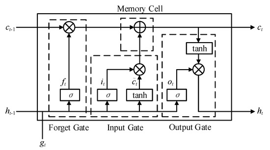
Figure 1.
Internal structure of long short-term memory (LSTM) unit.
The calculation formulas among the variables in Figure 1 are described as follows:
where , , , , , , and are respectively the forget gate, input gate, output gate, memory cell state, memory cell candicate state, input vector and the output vector at the current moment; and are respectively the memory cell state and the output vector at the previous moment, , , , are the weight matrices; , , , are the bias vectors; is the Hadamard product; and is the sigmoid function, which is mathematically described as
Multiple LSTM layers are stacked and connected to dense layers to form a complete LSTM network. If used as a regressor, the number of neurons in the output layer and whether the output layer employs an activation function depends on the target variable. If used as a binary classifier, the output layer contains only 1 neuron, and the class probability output is achieved after the sigmoid transformation shown in Equation (8).
where is the weight vector connected to the output layer, is the output vector of the previous layer, is the prediction probability of the model output, and in this paper, it refers to the transient instability probability.
2.2. Snapshot Ensembling Strategy
Constructing a reasonable ensemble model can effectively integrate the different mappings learned by each base model, and further improve the overall prediction performance. However, the time-consuming and computational cost of the general ensemble learning method is too high, which hinders its application in engineering practice [12]. In this paper, the snapshot ensembling [18] strategy is adopted to quickly integrate multiple different LSTM networks without increasing memory overhead.
For a neural network with a given structure, its weight parameter combination can be regarded as a point in a high-dimensional weight space, so there are infinite multiple weight combinations for any network structure. The process of training the network through the stochastic gradient descent (SGD) algorithm is essentially searching for the parameter combination corresponding to the lowest point of the loss function hypersurface, that is, the global optimal solution. Due to the non-convexity of the loss function, there are often multiple local optima on the hypersurface, and the deep neural network usually adopts optimizer such as Adam [19] to adjust the learning rate adaptively to avoid falling into local optima. However, the local optimal solution models are not meaningless. They learn the internal rules of data from different perspectives, and to some extent, they capture the representations that are ignored by the global optimal solution model. Snapshot ensembling strategy introduces a cyclic cosine annealing learning rate schedule to SGD to explore multiple local minima in the loss hypersurface. The expression of the learning rate is
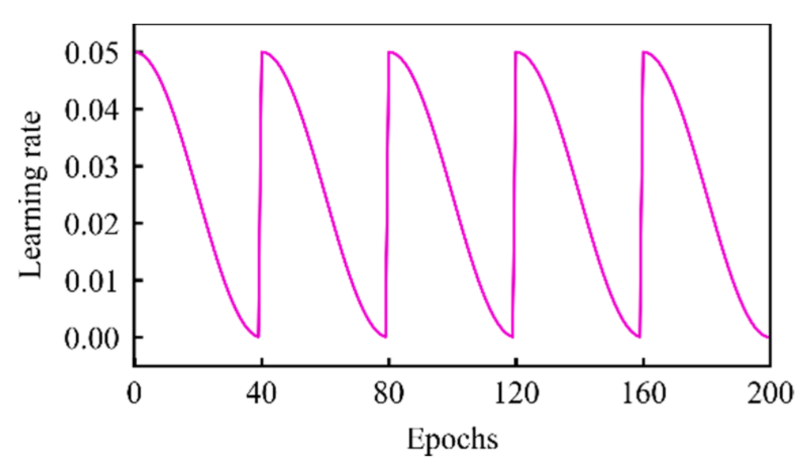
where j is the iteration times, is the initial learning rate, J is the total number of iterations during training, C is the cosine annealing cycles. In order to visually show the change curve of the learning rate with cosine annealing, set , , and , and the learning rate schedule is shown in Figure 2.
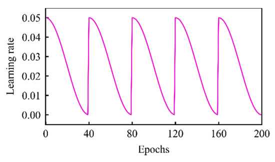
Figure 2.
Cyclic cosine annealing learning rate schedule.
As shown in Figure 2, with the increase of epochs, the learning rate fluctuates sharply and cyclically. At the beginning of the training process, due to the sharp drop in the learning rate, SGD will quickly converge to a local minimum in the loss hypersurface, and take a snapshot to add the model of the current node to the collection. After the snapshot is completed, SGD is warm restarted with a large initial learning rate, escapes the current local minimum, and starts the exploration of the next local minimum. Through this mechanism, the SGD propagation process will collect multiple local optimal models to achieve ensemble learning. Because the mapping relationships established by different weight combinations of the network are different, the diversity of the base learners is ensured, and the ensemble model will show better performance.
Unlike traditional ensemble learning that requires repeated construction of sub-models for training, snapshot ensembling can generate multiple models in the same training process, saving a lot of time and computing power. When electrical power equipment overhaul and other factors cause changes in the grid topology, or regular maintenance, the snapshot ensemble TSA model can be quickly adjusted to complete the update of the network weight, and put into online implementation in time.
2.3. Optimal Weighted Combination Method
After generating a series of base learners through snapshot ensembling, it is necessary to combine their prediction results into one through a certain combination strategy. In this paper, the error reciprocal method is adopted to carry out a weighted combination of each base learner, and the calculation formula of the weight coefficient is
where M is the number of base learners, is the weight coefficient of the m-th base learner, N is the total number of training samples, and is the error of the m-th base learner on the i-th training sample.
Therefore, the final prediction result of the ensemble model can be expressed as
where and are the prediction results output by the ensemble model and the m-th base learner, respectively.
Combining Equations (10) and (11), it can be seen that the base learner with a smaller error will be given a larger weight coefficient. After model integration, the deviations of the base learners in different directions will be offset with each other, and the overall prediction accuracy will be further improved.
3. Proposed Model for TSA
3.1. Two-Stage Assessment Mechanism Based on Classification and Regression
3.1.1. Hierarchical Real-Time Classification Framework
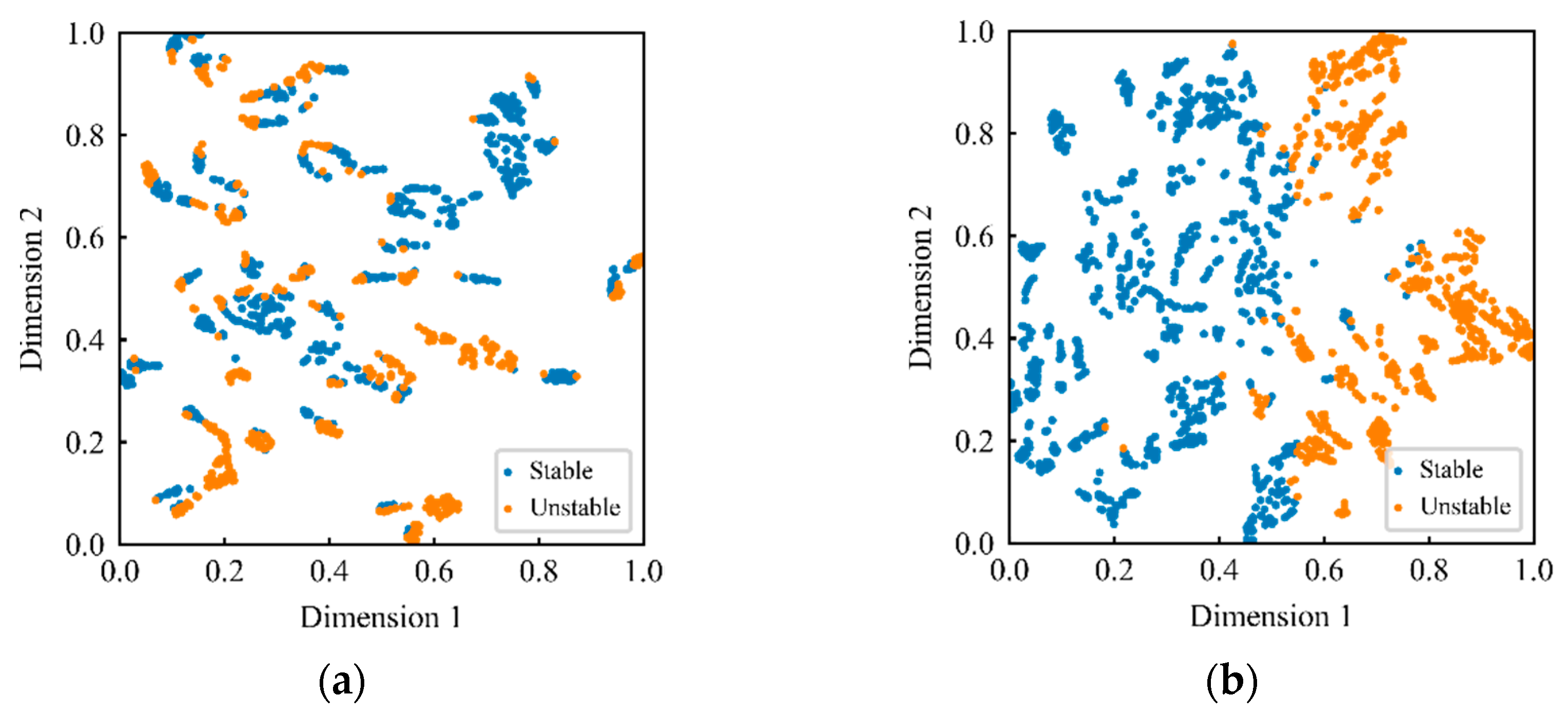
In the actual dynamic monitoring of the power system, the real-time measurement data transmitted by PMUs to the dispatching and communication center is continuously accumulated, which contains a wealth of dynamic trajectory information of the power grid. Based on the recursive structure of LSTM, a sliding time window is constructed to select the sub-sequences of the real-time disturbed trajectory measurements as the inputs of the classifier, which can realize the continuous hierarchical assessment process. As shown in Figure 3, it is the active power output data set obtained from generator 30 in the New England 39-bus system under various load levels. Figure 3a,b respectively correspond to the distribution of data in stable and unstable conditions under different response times, and the data have been normalized.
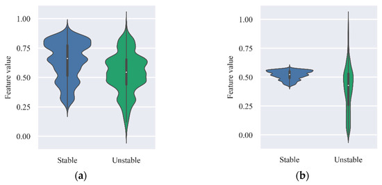
Figure 3.
Distribution of feature in stable and unstable conditions: (a) the 1st cycle after fault clearance; (b) the 50th cycle after fault clearance.
If the distribution of a feature in two different classes is similar, the correlation between the feature and the predicted target variable is weak. It can be seen from Figure 3a that the data distributions in stable and unstable conditions are highly similar. It can be seen from Figure 3a that the data distributions under stable and unstable conditions are highly similar, indicating that the feature has a weak correlation with transient stability in the early stage after fault clearance. In contrast, Figure 3b shows the distributions of data in two different conditions at the 50th cycle after fault clearance. The comparison shows that the electrical features have strong time-varying characteristics, and as time goes by, the correlation between the features and the transient stability of the system will become stronger. Therefore, in the hierarchical assessment process, the reliability of the prediction results output by the ensemble LSTM classifier is improved step by step. Similar to the confidence index proposed by [11], this paper defines the credibility index R to measure the reliability of the prediction results, and its expression is
where is the probability that the classifier predicts that x is an unstable sample, is the probability that the classifier predicts that x is an stable sample. Obviously, .
In order to gradually screen out credible samples, set credible instability threshold and credible stability threshold to and respectively. When , if , the instance is judged to be credible stable, otherwise it is marked as undetermined. When , if , the instance is judged to be credible unstable, otherwise it is marked as undetermined. When entering the next round of assessment cycle, the real-time trajectory measurements corresponding to the undetermined sample are dynamically extended, the time window slides forward to update the time series data, and then the data is input into the ensemble LSTM classifier to determine again until the specified upper limit of response time is reached. The transient information contained in the early response trajectory measurements corresponding to some critical samples is not rich, and it is difficult for the classifier to distinguish them reliably. However, the potential connection between trajectory information and transient stability will continue to strengthen and develop, and the classifier will output more reliable prediction results in the next round of assessment.
3.1.2. Stability Margin Prediction and Risk Quantification
On the one hand, for samples that are still marked as undetermined by the ensemble LSTM classifier after reaching the specified upper limit of response time, they need to be judged again through the second line of defense. On the other hand, for samples that are judged to be credible stable, it is necessary to further obtain their transient stability margins to provide a more targeted reference for subsequent power system dispatching and control. Therefore, for the above two types of samples, this paper constructs an ensemble LSTM regressor to quantitatively predict their transient stability margins. If the assessment result is instability, early warning should be given as soon as possible, and dispatchers can make timely adjustments and decisions.
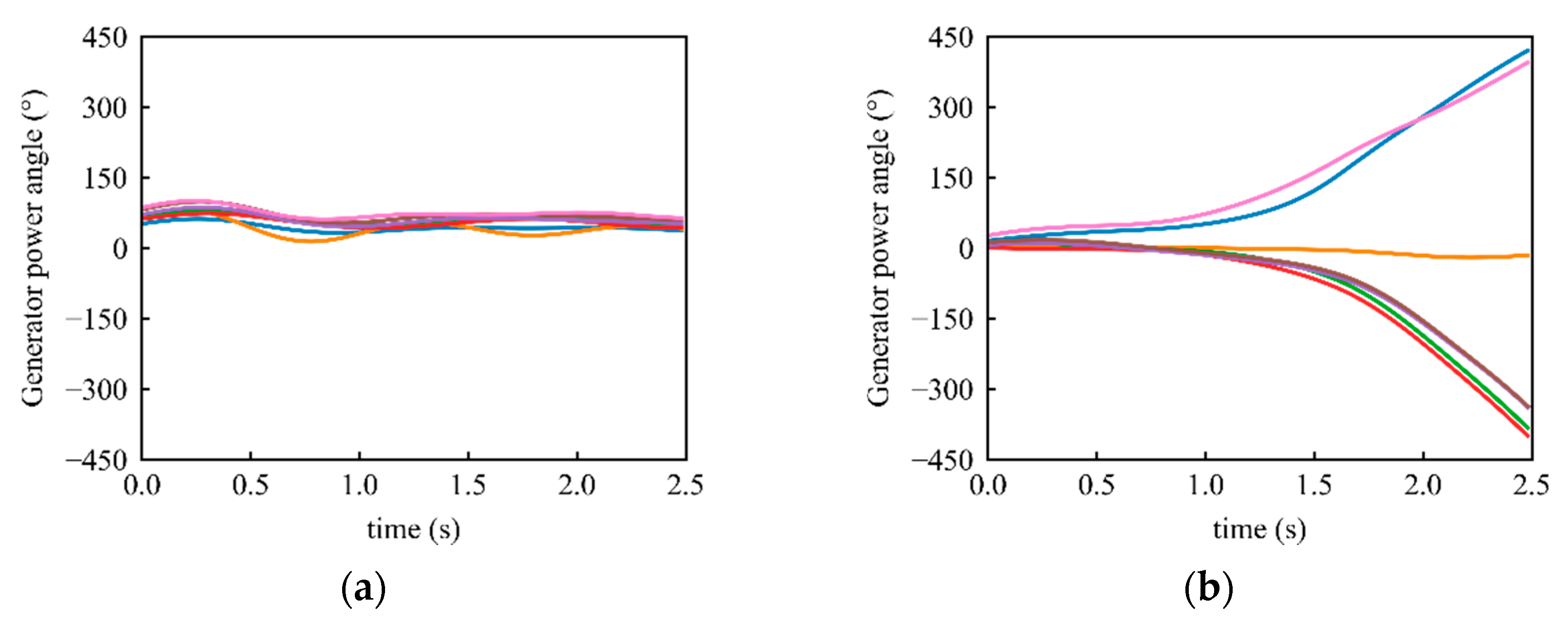
References [20,21] construct the transient stability margin index of the power system based on CCT. However, CCT needs to be tested repeatedly to determine through multiple time-domain simulations, which is cumbersome and extremely time-consuming for a large number of samples, and is difficult to be applied in actual large-scale power grids. The post-disturbance dynamic response curves of generator power angles in a power system under different operation conditions are shown in Figure 4. It can be seen that the variation of generator power angles can directly and effectively reflect the transient stability status of the power grid.

Figure 4.
Post-disturbance dynamic response curves of generator power angles corresponding to different stability status: (a) transient stable; (b) transient unstable.
Therefore, this paper defines TSI [22] as Equation (13), and employs it as the target variable predicted by the ensemble LSTM regressor.
where refers to the maximum power angle difference between any two generators in the system. Obviously, . When , the system is unstable. When , the system is stable, and the greater TSI, the greater the transient stability margin of the system.
Although TSI can quantitatively reflect the stability margin of the system, it is not refined enough in terms of risk indication. Therefore, it is necessary to construct a reasonable risk function and classify the risks so that the dispatcher can take more specific subsequent control measures.
The strong nonlinearity and non-autonomy of the power system determine the nonlinearity of the risk function. As TSI decreases, its corresponding risk indicators should rise faster and faster. Therefore, this paper adopts an exponential utility function to describe the degree of risk. The risk function S should consider both the system’s transient stability probability and the severity of failure [23], so this paper defines the risk factor: . Set the threshold , when , the system is considered to be hyperstable, S = 0. When , the system is considered to be unstable, S = 3. When , the risk function expression is
where A and B are coefficients.
Since the risk function is a continuous function, substituting the coordinates (,0) and (0,3) into Equation (14), the risk function on the domain can be obtained as
In the process of dynamic security monitoring of the actual power grid, dispatchers should not only pay attention to the instability situation, but also pay attention to the high-risk situations near the stability domain boundary, and formulate preventive control measures in time to improve the stability of the system. This paper divides the risk into the following five ranks
where denotes the risk rank of the power grid, and and are the thresholds for grading risk, which need to be set reasonably according to the security risk specification requirements and sample conditions of the actual power grid. means the system is hyperstable and there is no risk of instability. means the system is basically stable and the risk of instability is low. means the system is weak-stable and the risk of instability is moderate. means the system is critical stable and the risk of instability is high. means the system will be unstable.
3.2. Input Features of Model
For data-driven TSA methods, the performance of model predictions largely depends on the selection of input features, so it is particularly critical to construct a set of features that can accurately reflect the dynamic behavior of the power system. Taking into account the strong abstract characterization ability of the LSTM network and the real-time nature of PMU data acquisition, this paper selects the real-time disturbed trajectories of underlying measurements as shown in Table 1 as the feature set, where n1, n2, n3, and n4 are respectively the number of bus, transmission lines, generators, and load nodes in the power grid, and s is the number of sampling times.

Table 1.
Input feature set.
Feature types 1 and 2 characterize the power supply and demand in the system, which are closely related to the operating conditions and fault conditions of the system. Feature type 3 can implicitly describe the topology information of the system [24], and Feature type 4 can reflect the dynamic changes of the system very quickly [25,26]. Each type of feature complements each other, cover all bus and lines in the power grid, and can comprehensively and quickly reflect the dynamic behavior of the power system.
The distribution of the underlying measurement data is usually skewed, and the dimensions of each electrical quantity are different. In order to improve the prediction performance and accelerate the convergence of the model, the raw measurement data needs to be preprocessed before being input to the model. First, perform Yeo-Johnson power transformation on the raw data, the calculation formula is
where and are the transformed pre-value and post-value of a feature in the sample sequence at time t respectively, is the transformation parameter, whose value is determined by the maximum likelihood estimation method.
Yeo-Johnson power transformation can correct the skewness of the raw feature data, convert a skew distribution to a Gaussian distribution, thereby improving the modeling accuracy. Next, perform Z-Score standardization on the data, the calculation formula is
where is the normalized value, and are the mean and standard deviation of feature data at time t after Yeo-Johnson power transformation, respectively.
All feature data in the sample set obeys the standard normal distribution after Z-Score standardization, which is in the same order of magnitude. Standardization can eliminate the influence of excessive numerical differences between the features of different dimensions on the learning of the ensemble LSTM model, and accelerate the algorithm convergence.
3.3. Network Structure of Model
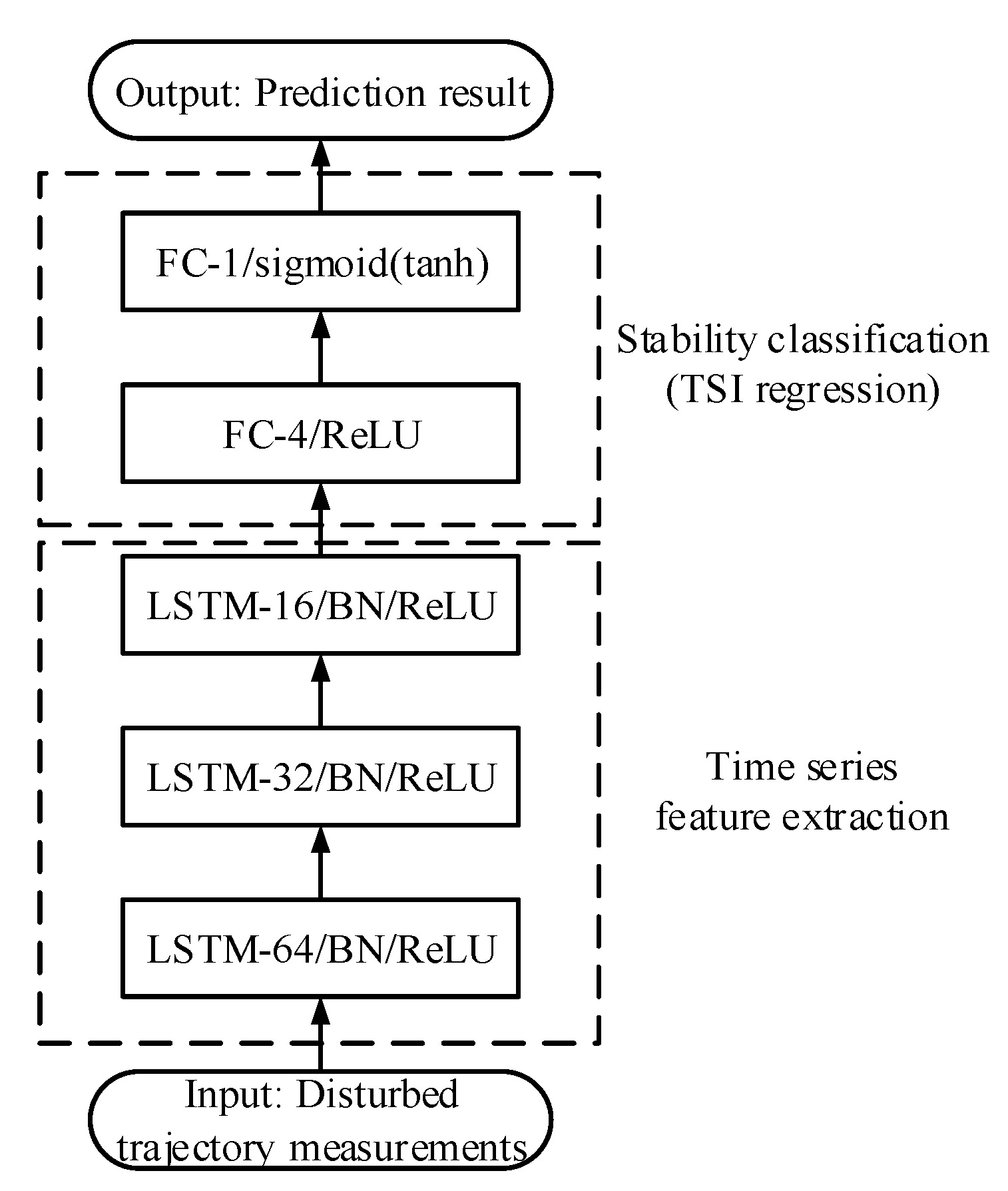
This paper constructs a five-layer network model as shown in Figure 5 as the base learner for TSA. In Figure 5, FC represents a fully connected layer, and BN represents batch normalization [27]. FC-1/sigmoid(tanh) means that the fully connected layer contains 1 neuron, and the activation function is sigmoid function (classifier) or tanh function (regressor). Similarly, LSTM-64/BN/ReLU means that the LSTM layer contains 64 neurons, the data is batch normalized before the activation function to facilitate gradient propagation, and the Rectified Linear Unit (ReLU) is employed as the activation function, where .
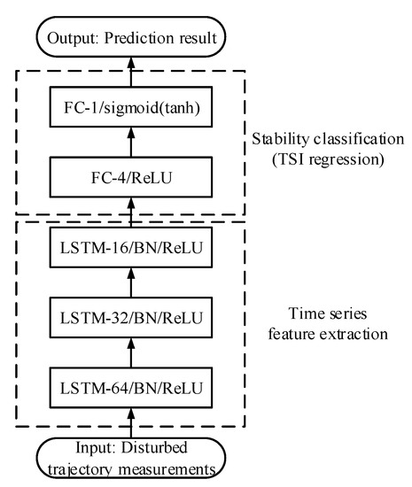
Figure 5.
Structure diagram of transient stability assessment (TSA) base model.
The first part of the model consists of 3 LSTM layers, and the number of neurons decreases layer by layer, which can realize the progressive extraction of abstract high-order features from the input time series data. After the time series passes through three LSTM layers, the feature data points are reduced from to 16. The latter part of the model is composed of two FC layers, which can establish a complex nonlinear mapping between advanced features and the classes or margins of power system transient stability.
In practical applications, the structural parameters of the LSTM network can be adjusted according to the specific scale of the power system, but it does not affect the subsequent analysis of the effectiveness of the proposed method.
3.4. Indicators for Performance Evaluation
In actual power system dispatching, the TSA model’s missing alarms for instability conditions will bring huge security hazards to the system, while the cost of false alarms for stable conditions is relatively small. Considering the different costs of misclassification of the two classes of samples in TSA, in addition to the conventional indicator accuracy , this paper also introduces the missing alarm rate and false alarm rate as evaluation indicators of the classifier. The confusion matrix of TSA is constructed as shown in Table 2, where TP and FP respectively denote the number of samples predicted by the classifier as unstable while actually labeled as unstable and stable, TN and FN respectively denote the number of samples predicted by the classifier as stable while actually labeled as stable and unstable.
Table 2.
Confusion matrix of transient stability assessment (TSA).
The calculation formulas for each evaluation indicator of the classifier are
Meanwhile, for the output of each stage of hierarchical prediction, this paper defines the indicator cumulative hit rate as Equation (22), which denotes the ratio of the number of credible samples output by the hierarchical model up to the current stage to the total number of test samples.
where is the total number of test samples, and are respectively the number of accumulatively identified credible stable samples and credible unstable samples.
For the transient stability margin regressor, the mean absolute error is employed as the evaluation indicator, and its expression is
where and are the actual and predicted values of TSI of the i-th test sample, respectively.
4. Improvements Considering Sample Imbalance and Overlapping
The essence of deep learning model training is to minimize the loss function through optimization algorithms. In the binary classification task of predicting whether the system is stable or not, the model usually employs cross entropy as the loss function, and its expression is
Due to the robustness and self-healing ability of modern smart grids, the power system can transition to a steady state by itself in most cases after the disturbance is cleared. In the actual power system TSA, there is a significant sample imbalance problem, which means that there are far more stable samples than unstable samples that can be used for model training. In order to minimize cross entropy during the training process, the model is more inclined to predict unknown samples as stable samples, thereby sacrificing the prediction accuracy of unstable samples.
Aiming at the problem of sample imbalance, the common improvement methods mainly include the following two:
- In terms of input data, undersampling, oversampling, and data augmentation are used to balance the ratio of the two classes of samples [28,29];
- In terms of algorithm, weighted cross entropy is employed to make the model cost-sensitive [8,12].
However, all of the above methods will lead to an increase in false alarm results, because another key factor that affects the performance of the model is not considered: there are some overlapping areas in the feature vector space of the two classes of samples [30], and the samples in these areas are called hard samples, and the TSA model’s prediction results for these samples have low credibility and difficult to classify. To solve this problem, [31] used SVM as the classifier, divided the feature space into credible area and incredible area according to the optimal separating hyperplane constructed by support vectors, and built several auxiliary classifiers as secondary criteria to identify the incredible area samples of the main classifier. However, this method cannot essentially improve the level of credibility of the prediction results of hard samples, and the choice of the main classifier lacks scientific guidance and is subjective, which makes it difficult to ensure that the prediction results are completely credible. Therefore, this paper makes improvements to the algorithmic defects of cross entropy to overcome the problem of sample imbalance and deepen the mining of hard samples.
It can be deduced from Equation (7) that . Substituting Equation (8) into Equation (24), the following can be obtained:
The expression of the modified cross entropy is
where and are the weight coefficient and the penalty coefficient, respectively.
By setting , the loss contribution of unstable samples can be improved, and the model’s sensitivity to the cost of unstable samples can be improved, thereby reducing missing alarms. In this paper, set , where and denote the number of stable samples and the number of unstable samples in the training set, respectively. Setting to a larger positive value enables hard samples to obtain a larger gradient than easy samples during SGD iteration, thereby correcting the optimization direction of the model. Take the unstable instance y = 1 as an example, the higher the instability probability (i.e., the larger ) given by the model for the unstable instance, the smaller the penalty factor . When is large enough, will be very close to 0, thereby reducing the loss contribution of easy samples in the model training process, making the model more focused on the mining of hard samples. The same is true for stable instances . In this paper, set .
5. Case Study
5.1. Test System and Data Generation
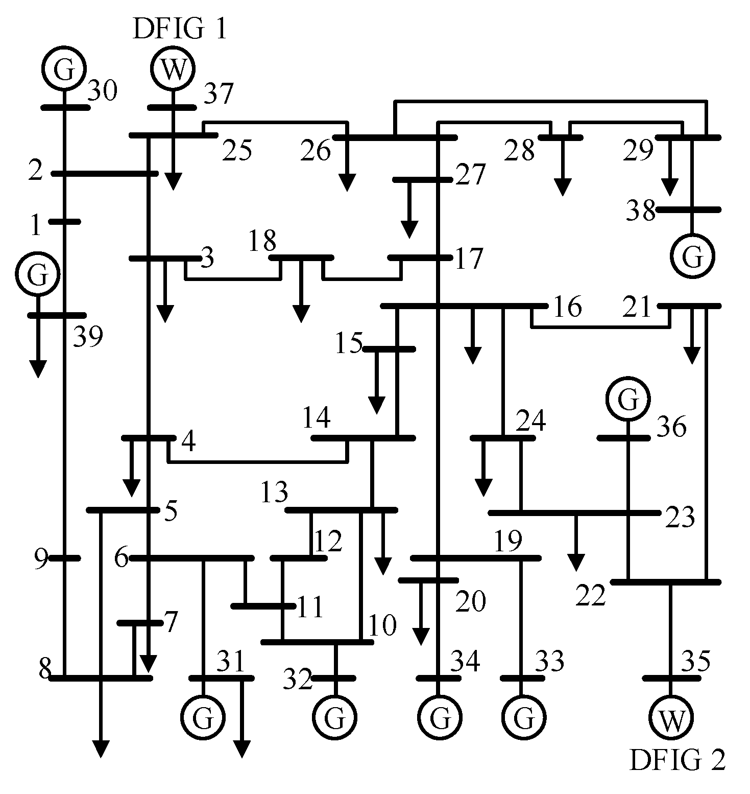
The New England 39-bus system integrated with wind farm is used as a test system to verify the effectiveness of the proposed method. The synchronous generators connected to bus 35 and bus 37 in the original system are replaced by doubly fed induction generators (DFIGs). The system consists of 8 synchronous generators, 2 DFIGs, 12 transformers, 39 bus, and 34 transmission lines, whose topology is shown in Figure 6.
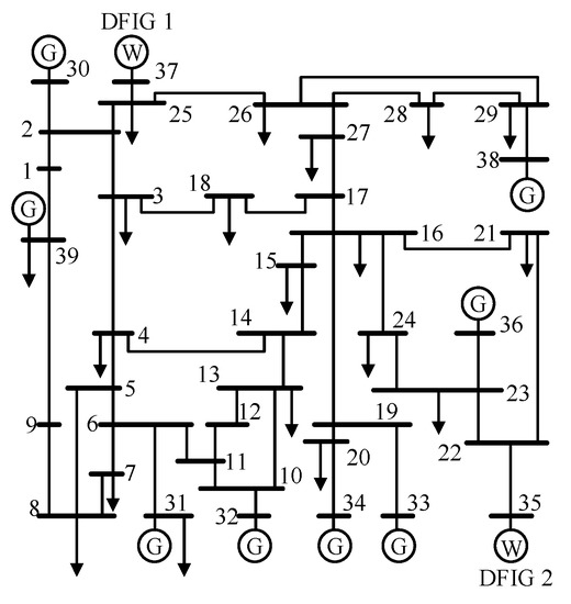
Figure 6.
Topology of the New England 39-bus system integrated with wind farm.
The time-domain simulations are conducted by PSD-BPA to generate an enormous database. The synchronous generators are set as fourth-order models and the loads are set as constant-impedance models. Each DFIG is set as GE wind power generator model, and its capacity is equal to that of the corresponding original synchronous generator. Detailed parameters of this system can be found in [32]. In order to generate a reasonable and comprehensive dataset, the operating conditions of the test system are randomly varied. Considering 10 different load levels of 80%, 85%, …, 125%, while adjusting the output of each synchronous generator to ensure the convergence of the power flow and the deviation of each bus voltage within 0.05 p.u. The output of each wind farm fluctuates randomly between 30% and 100% of its rated capacity, and the variation of load and wind farm output are shared by synchronous generators in proportion to their rated capacity. The contingencies are mainly three-phase permanent short-circuits at each bus and 5 locations (20%, 35%, 50%, 65%, and 80% lenth) of each transmission line. The failure duration is set from 120 to 220 ms with a step length of 20 ms. The simulation time is 6 s, and the sampling frequency is 60 Hz. Finally, a total of simulation results can be generated, including 7419 stable samples and 4821 unstable samples. Using stratified random sampling, all samples are divided into training set, validation set, and test set at a ratio of 3:1:1 to ensure the same ratio of stable/unstable samples in each set. The test set is completely unknown during the offline training of the TSA model, which is used to simulate real-time input data during online prediction.
5.2. Effectiveness Analysis of Ensembling Strategy
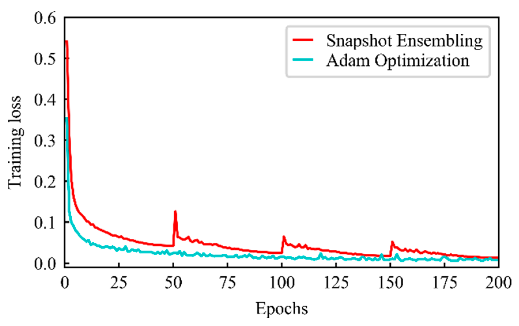
The length of the sliding time window is set to 10 cycles. The following discussion takes the sampling interval as the first 10 cycles after fault clearance and the classifier with a classification threshold of 0.5 as an example to discuss the effectiveness and feasibility of the proposed method. The hyperparameters of the proposed snapshot ensemble LSTM network can be mainly divided into three types: structural parameters, loss function parameters and learning rate parameters. The first two types of hyperparameters have been given above, and the learning rate parameters in Equation (9) are set as follows: , and . In order to intuitively compare the differences in the training process between the cyclic cosine annealing learning rate schedule and the typical learning rate schedule, an LSTM network with the same structure using the Adam optimizer is established. The training process of the two models is shown in Figure 7.
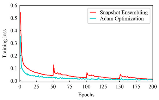
Figure 7.
Learning curves of long short-term memory (LSTM) networks.
In Figure 7, the red line denotes the snapshot ensembling, and the cyan line denotes the Adam optimization with standard learning rates. It can be seen from Figure 7 that the optimal loss values that the two curves converge to at the end of training are almost the same, but the training processes of the two are quite different. The training loss value in the early stage of the cyan line drops rapidly, and slowly decays after about 10 epochs, and the curve is relatively flat. The evolution trend of the red line presents a state of twists and turns, and the corresponding loss function values fall into 4 different local minima at the 50th, 100th, 150th, and 200th epochs. After reaching a local minima, the curve quickly rises and then drops again, showing a certain periodicity. In summary, the cyclic fluctuations of the cosine annealing learning rate can enable gradient descent to obtain a larger exploration domain on the loss hypersurface, so as to traverse and collect multiple local optimal models.
In order to verify the effectiveness of the adopted ensembling strategy, the snapshot ensemble LSTM classifier and each LSTM base classifier (respectively denoted as LSTMa, LSTMb, LSTMc, LSTMd) are tested and compared on the same test set. The prediction results are shown in Table 3.
Table 3.
Prediction results of different long short-term memory (LSTM) classifiers.
It can be seen from Table 3 that the PACC of each LSTM classifier is above 99%, indicating that the LSTM network has a powerful multivariate time series data mining capability, which is highly adaptable to high-dimensional, time-varying, and strongly nonlinear power system data. The PMAR and PFAR of the ensemble LSTM classifier are both lower than that of any base classifier, with the highest prediction accuracy, which indicates that snapshot ensemble LSTM can effectively integrate the diversity of each base learning, further improve the prediction accuracy and generalization ability, and verify the effectiveness of the integration strategy used. From the results, the effectiveness of the adopted ensembling strategy is verified.
5.3. Visual Analysis of Feature Extraction
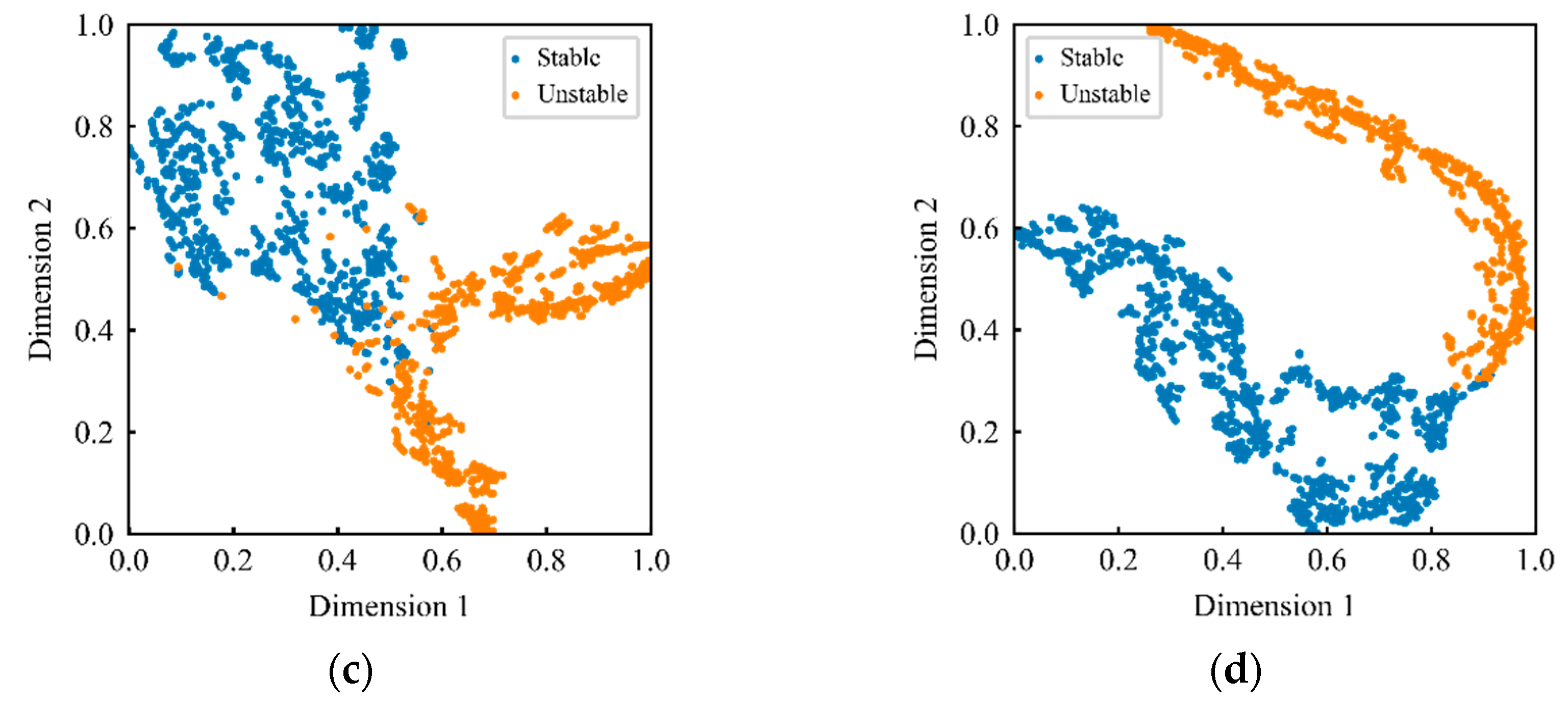
T-distributed stochastic neighbor embedding (t-SNE) [33] is a nonlinear data dimensional reduction algorithm that can project data sets in a high-dimensional Euclidean space into a two-dimensional or three-dimensional embedding space to realize data visualization while retaining a large amount of original information. In order to visually show the progressive representation learning process of the LSTM network for the underlying temporal features, this paper uses the t-SNE algorithm to project the original data of the test set and the output of each LSTM layer onto a two-dimensional plane. The visualization results are shown in Figure 8.
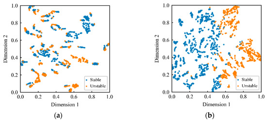
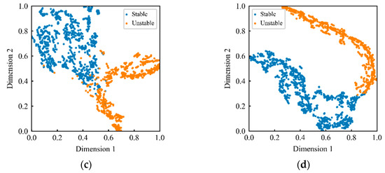
Figure 8.
Visualization results based on t-distributed stochastic neighbor embedding (t-SNE): (a) original input; (b) output of the first LSTM layer; (c) output of the second LSTM layer; (d) output of the third LSTM layer.
It can be seen from Figure 8a that the distribution of samples in the original feature space is highly discrete, and stable samples and unstable samples are doped and overlapped with each other, which makes it difficult to demarcate an ideal stable boundary. According to Figure 8b–d, it is shown that as the network deepens, samples of different classes are gradually separated, forming more and more obvious clusters. After completing the feature extraction of LSTM layers three times in sequence, a clear boundary has appeared between the two classes of sample sets, showing a nearly linearly separable distribution state.
As explained above, the LSTM network has a strong temporal feature extraction capability. By performing multi-level information distillation on the original input data, it can transform advanced features that are strongly related to transient stability, thereby realizing effective transient stability prediction.
5.4. Performance Comparison with Other Kinds of Classifiers
In order to further verify the superiority of the proposed model, the deep learning classifiers deep belief network (DBN) and CNN, as well as the commonly used shallow learning classifiers SVM and decision tree (DT) are built on the same data set as baseline models. The DBN network adopts a four hidden-layer structure, and the number of neurons in each hidden layer is 500-200-80-20. The CNN network consists of two convolutional layers, two pooling layers, and two fully connected layers, and the convolution kernel length is 3. SVM adopts radial basis function as the kernel function, and its optimal hyperparameter combination is determined by grid search combined with five-fold cross-validation. DT adopts C5.0 algorithm. Except for snapshot ensemble LSTM and CNN, the other model inputs are required to be one-dimensional vectors, so each time series matrix in the sample set is flattened to one dimension according to the time dimension to fit the corresponding classifiers. The performance of each model on the test set is shown in Table 4.
Table 4.
Test results of different kinds of classifiers.
It can be seen from Table 4 that the comprehensive prediction performance of the deep learning models CNN, DBN, and ensemble LSTM is better than that of the shallow learning models SVM and DT. The results show that the deep network structure can effectively extract more generalized data representations from the underlying features, and then establish a more accurate nonlinear mapping. Furthermore, after the multivariate time series is flattened into a one-dimensional array, the dynamic change characteristics of the electrical quantity in the continuous time section are buried, and DBN cannot perceive the timing feature information from a large number of data points, so the overall performance has a certain gap compared with CNN and ensemble LSTM. As a common model for processing sequence data, CNN’s PACC on the test set reaches 98.53%. However, due to the lack of consideration of the long-term dependence of the disturbed trajectory data and the single network mapping rule, CNN is not as accurate as ensemble LSTM in prediction.
On the whole, the ensemble LSTM classifier achieved the best performance in all three indicators, with PACC as high as 99.59%, PMAR and PFAR only 0.41% and 0.40%. This shows that the ensemble LSTM network can fully mine the transient information in the time series trajectories, and the identification ability of the two classes of samples is relatively balanced.
5.5. Impact of Loss Function Modification on Hierarchical Prediction
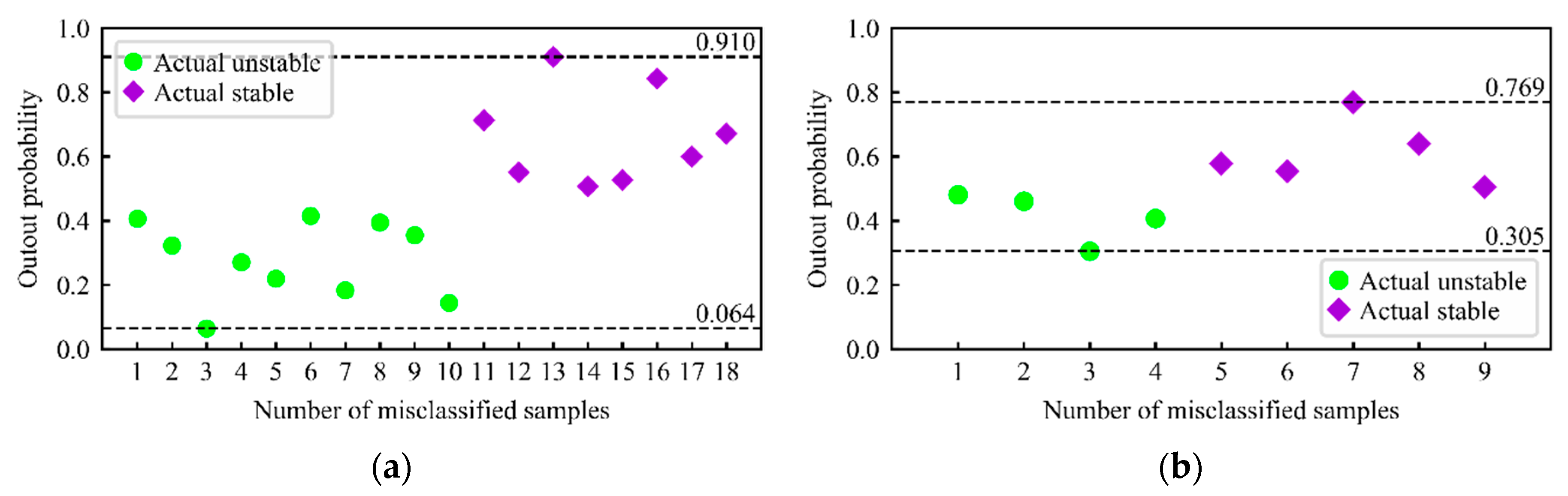
In order to verify the effectiveness and necessity of loss function modification, LSTM classifier with cross entropy (abbreviated as CE-LSTM) and LSTM classifier with modified cross entropy (abbreviated as MCE-LSTM) are built by snapshot ensembing under the condition that the other hyperparameters remained the same, and a comparative test of hierarchical prediction is performed. In the continuous hierarchical prediction process, the credibility threshold is a criterion to measure the reliability of the prediction result, and the values of and need to be determined according to the prediction results of the classifier on the validation set. Figure 9 shows the probability output of misclassified samples on the validation set of two ensemble LSTMs with different loss functions.
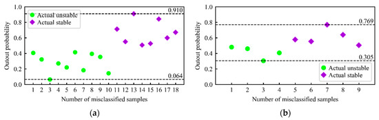
Figure 9.
Output probability distribution of misclassified samples: (a) ensemble CE-LSTM; (b) ensemble MCE-LSTM.
It can be seen from Figure 9a that if the value of is set to be greater than 0.910, ensemble CE-LSTM will not output false alarm results, so the results predicted to be transient unstable are credible; if the value of is set to be greater than 0.936, i.e., 1 − 0.064, ensemble CE-LSTM will not output missing alarm results, so the results predicted to be transient stable are credible. Similarly, it can be seen from Figure 9b that the values of and of ensemble MCE-LSTM should be set to be greater than 0.769 and 0.695, respectively. Comparing Figure 9a,b, it can be seen that after the modification of cross entropy, not only the misjudgment of the classifier is reduced, but also the probability distribution interval of the misclassified samples is significantly reduced, which indicates that ensemble MCE-LSTM has stronger generalization ability.
In order to make the established ensemble LSTM classifier universal in each stage of hierarchical evaluation, a 10-cycle time window is slid along the time dimension, so that the sequence in the sample set is sub-sampled multiple times and preprocessed as the model inputs. In order to reduce the randomness of model training, the credibility threshold is set and verified through 10-fold cross-validation, and some margin is left to ensure the conservativeness of the prediction. For ensemble CE-LSTM, and are set to 94.75% and 96.82%, respectively. For ensemble MCE-LSTM, and are set to 80.84% and 75.17%, respectively. In order to ensure the rapidity of TSA, the upper limit of response time is specified as 30 power frequency cycles, i.e., 0.5 s. The comparative test results of hierarchical prediction are shown in Table 5.
Table 5.
Comparative test results of hierarchical prediction.
As can be seen from Table 5, ensemble MCE-LSTM can accurately determine more than 90% of the samples in the first cycle. As time goes by, the undetermined samples are gradually identified. When the response time reaches 30 cycles (0.5 s), ICHR of MCE-LSTM has risen to 99.14%. This shows that the evolution of time series features can fully reflect the dynamic behavior of the system in the transient process, and the ensemble LSTM model has a deeper grasp of the development trend of the system, so as to reliably identify more critical samples gradually. After verification, it is found that by the 30th cycle, the TSI values of the remaining uncertain samples are all close to 0, which belong to the critical stable or critical unstable samples. Among them, the instability occurrence time of the unstable samples all exceeds 3 s, and there are multi-swing instability conditions. Therefore, ensemble MCE-LSTM can quickly screen out faults that are far from the boundary of the stability region, and can also reserve enough time margin for the very small number of uncertain critical samples, so as to facilitate the quantitative risk assessment in the second stage and subsequent emergency control. In addition, ensemble MCE-LSTM is always ahead of ensemble CE-LSTM in terms of ICHR indicator in the assessment process, indicating that after the modification of cross entropy, the model can more fully mine hard samples, which further improves the sensitivity and rapidity of hierarchical prediction.
5.6. Risk Quantification of Transient Angle Stability
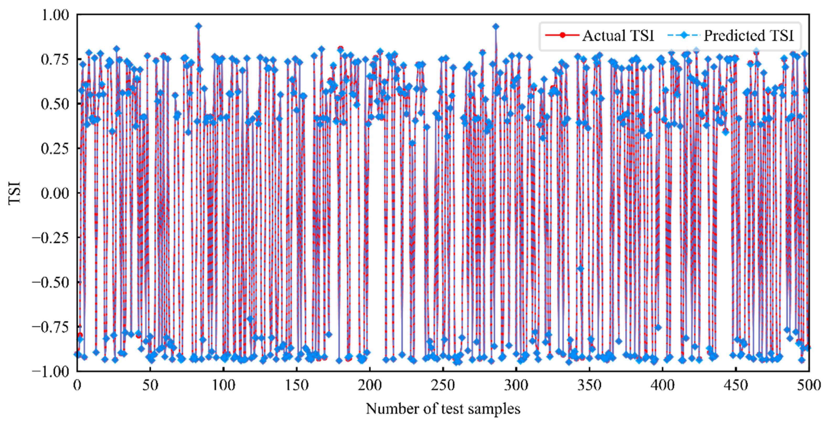
The modeling process of the snapshot ensemble LSTM regressor is similar to the snapshot ensemble LSTM classifier, but the mean square error is adopted as the loss function. 500 samples from the test set are randomly selected for visualization, and the curves of the true and predicted TSI values are shown in Figure 10.
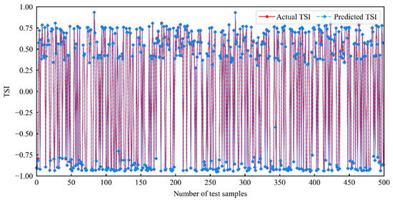
Figure 10.
Regression prediction results of transient stability index (TSI).
As can be seen from Figure 10, the predicted value curve of TSI by snapshot ensemble LSTM regressor is highly consistent with the actual value curve, and has a synchronized change trend. After calculation, of the regressor on the entire test set is only 0.00183, and the prediction accuracy is high enough to meet the requirements of practical assessment application.
Furthermore, according to the TSI prediction results and the transient stability probability prediction results of the samples, the risk grading of transient angle stability can be realized. The thresholds , , and are set to 0.8, 0.5, and 1, respectively. According to Equations (15) and (16), the risk grading results of the samples are shown in Table 6.
Table 6.
Risk grading results of each sample set.
Comparing and analyzing the risk grading results in Table 6 and the time-domain simulation settings corresponding to the samples, it is found that the risk grading results are consistent with the actual operating experience of power systems. That is to say, under some operation modes such as heavy load on some grid nodes, some transmission line power flows close to the power transfer limit, and a long fault duration, the transient stability probability and TSI predicted by the TSA models are low, corresponding to high risk ranks 3 and 4, and vice versa.
The risk grading obtained by combining the predicted results of the proposed TSA models and the risk function is essentially a quantitative analysis based on big data statistics. It can effectively overcome the subjectivity and incompleteness of manual experience grading, better reflect the transient safety risk level of power system, and provide an important reference for the risk management and control of power grid.
6. Conclusions
In order to make full use of the time series data sampled by PMUs and overcome sample imbalance and overlapping, this paper proposed a two-stage power system TSA method based on real-time disturbed trajectory measurements and snapshot ensemble LSTM network. Through the simulation experiments on the New England 39-bus system integrated with wind farm and the analysis of the case results, the following conclusions were drawn:
- The proposed snapshot ensemble LSTM network can effectively collect multiple global and local optima corresponding base models obtained in a single training process. Through the weighted combination of each base model, the obtained ensemble model can output more accurate predictions. LSTM network has stronger representation learning ability for transient stability temporal information, and can effectively extract higher-level abstract features with better separability from the original input, so the proposed model has higher prediction accuracy than other machine learning classifiers.
- Through the proper setting of credibility thresholds, it can effectively prevent the missing and false alarms during the hierarchical assessment process. As time goes by, the credibility of the prediction results gets higher and higher, so the critical samples are gradually and reliably identified. Moreover, the improvement of the loss function for sample imbalance and overlapping further improves the credibility of the model output and reduces misclassification.
- The built ensemble LSTM regression model can predict the transient stability margin accurately. Combined with the two-stage prediction output of classifier and regressor, the risk grading of transient angle stability can be further realized according to the established risk function, which is instructive for the subsequent risk control.
In future work, we will conduct in-depth analysis on the robustness of the proposed model in the case of partial measurement data missing caused by PMU failure and measurement data containing noise. Meanwhile, further verification of the proposed method with actual large-scale power grids as cases is also the work to be performed in the future.
Author Contributions
The authors confirm their contributions to the paper as follows: Y.D. proposed the idea, performed the experiments, analyzed the data and wrote the paper; Z.H. provided useful advice, revised the manuscript, and approved the final version of the manuscript. Both authors have read and agreed to the published version of the manuscript.
Funding
This research was funded by the National Natural Science Foundation of China, grant No. 51977156.
Conflicts of Interest
The authors declare no conflict of interest.
Nomenclature
| Parameters | |
| weight matrices | |
| bias vectors | |
| weight vector connected to the output layer | |
| initial learning rate | |
| total number of iterations during training | |
| cosine annealing cycles | |
| number of base learners and training samples | |
| weight coefficient of the m-th base learner | |
| credible instability threshold and the credible stability threshold | |
| risk factor threshold | |
| coefficients in the risk function | |
| thresholds for grading risk | |
| number of bus, transmission lines, generators and load nodes | |
| number of sampling times. | |
| total number of test samples | |
| weight coefficient and the penalty coefficient | |
| number of stable samples and unstable samples in the training set | |
| Variables | |
| forget gate, input gate, and output gate at time t | |
| memory cell state and memory cell candicate state at time t | |
| input vector and the output vector at time t | |
| output vector of the previous layer of the output layer | |
| prediction probability of the model output | |
| learning rate in the j-th iteration | |
| error of the m-th base learner on the i-th training sample | |
| prediction probability output by the ensemble model and the m-th base learner | |
| credibility index | |
| transient stability index | |
| maximum power angle difference between any two generators in the system | |
| risk factor | |
| risk function value | |
| risk rank | |
| transformed pre-value and post-value of a feature at time t | |
| normalized and post-value of a feature at time t | |
| mean and standard deviation of feature data | |
| number of accumulatively identified credible stable samples | |
| number of accumulatively identified credible unstable samples | |
| cross entropy loss function | |
| modified cross entropy loss function | |
| Indicators | |
| accuracy | |
| missing alarm rate | |
| false alarm rate | |
| cumulative hit rate | |
| mean absolute error | |
References
- Zadkhast, S.; Jatskevich, J.; Vaahedi, E. A Multi-Decomposition Approach for Accelerated Time-Domain Simulation of Transient Stability Problems. IEEE Trans. Power Syst. 2015, 30, 2301–2311. [Google Scholar] [CrossRef]
- Chang, H.D.; Chu, C.C.; Cauley, G. Direct stability analysis of electric power systems using energy functions: Theory, applications, and perspective. Proc. IEEE 1995, 83, 1497–1529. [Google Scholar] [CrossRef]
- Zhu, Q.M.; Chen, J.F.; Zhu, L.; Shi, D.Y.; Bai, X.; Duan, X.Z.; Liu, Y.L. A Deep End-to-End Model for Transient Stability Assessment with PMU Data. IEEE Access 2018, 6, 65474–65487. [Google Scholar] [CrossRef]
- Zhang, Y.C.; Markham, P.; Xia, T.; Chen, L.; Ye, Y.Z.; Wu, Z.Y.; Yuan, Z.Y.; Wang, L.; Bank, J.; Burgett, J.; et al. Wide-Area Frequency Monitoring Network (FNET) Architecture and Applications. IEEE Trans. Smart Grid. 2010, 1, 159–167. [Google Scholar] [CrossRef]
- De La Ree, J.; Centeno, V.; Thorp, J.S.; Phadke, A.G. Synchronized Phasor Measurement Applications in Power Systems. IEEE Trans. Smart Grid. 2010, 1, 20–27. [Google Scholar] [CrossRef]
- Li, X.; Zheng, Z.Y.; Wu, L.H.; Li, R.Y.; Huang, J.Q.; Hu, X.L.; Guo, P.F. A Stratified Method for Large-Scale Power System Transient Stability Assessment Based on Maximum Relevance Minimum Redundancy Arithmetic. IEEE Access 2019, 7, 61414–61432. [Google Scholar] [CrossRef]
- Geeganage, J.; Annakkage, U.D.; Weekes, M.A.; Archer, B.A. Application of Energy-Based Power System Features for Dynamic Security Assessment. IEEE Trans. Power Syst. 2015, 30, 1957–1965. [Google Scholar] [CrossRef] [Green Version]
- Li, B.Q.; Wu, J.Y.; Hao, L.L.; Shao, M.Y.; Zhang, R.Y.; Zhao, W. Anti-Jitter and Refined Power System Transient Stability Assessment Based on Long-Short Term Memory Network. IEEE Access 2020, 8, 35231–35244. [Google Scholar] [CrossRef]
- Ren, C.; Xu, Y.; Zhang, Y.C. Post-disturbance transient stability assessment of power systems towards optimal accuracy-speed tradeoff. Prot. Control. Mod Power Syst. 2018, 3, 194–203. [Google Scholar] [CrossRef] [Green Version]
- Yin, X.Y.; Liu, Y.T. Deep Learning Based Feature Reduction for Power System Transient Stability Assessment. In Proceedings of the TENCON 2018—2018 IEEE Region 10 Conference, Jeju, Korea, 28–31 October 2018; pp. 2308–2312. [Google Scholar]
- Zhou, Y.Z.; Wu, J.Y.; Yu, Z.H.; Ji, L.Y.; Hao, L.L. A Hierarchical Method for Transient Stability Prediction of Power Systems Using the Confidence of a SVM-Based Ensemble Classifier. Energies 2016, 9, 778. [Google Scholar] [CrossRef] [Green Version]
- Zhou, Y.Z.; Guo, Q.L.; Sun, H.B.; Yu, Z.H.; Wu, J.Y.; Hao, L.L. A novel data-driven approach for transient stability prediction of power systems considering the operational variability. Int. J. Electr. Power Energy Syst. 2019, 107, 379–394. [Google Scholar] [CrossRef]
- Mi, D.K.; Wang, T.; Xiang, Y.W.; Du, W.J. Elastic Net based online assessment of power system transient stability margin. Power Syst. Technol. 2020, 44, 19–26. [Google Scholar]
- Zhang, R.Y.; Wu, J.Y.; Xu, Y.; Li, B.Q.; Shao, M.Y. A Hierarchical Self-Adaptive Method for Post-Disturbance Transient Stability Assessment of Power Systems Using an Integrated CNN-Based Ensemble Classifier. Energies 2019, 12, 3217. [Google Scholar] [CrossRef] [Green Version]
- Yin, X.Y.; Yan, J.C.; Liu, Y.T.; Qiu, C.G. Deep learning based transient stability assessment and severity grading. Electr. Power Autom. Equip. 2018, 38, 64–69. [Google Scholar]
- Yu, J.J.Q.; Hill, D.J.; Lam, A.Y.S.; Gu, J.T.; Li, V.O.K. Intelligent Time-Adaptive Transient Stability Assessment System. IEEE Trans. Power Syst. 2018, 33, 1049–1058. [Google Scholar] [CrossRef] [Green Version]
- Yu, J.J.Q.; Lam, A.Y.S.; Hill, D.J.; Li, V.O.K. Delay Aware Intelligent Transient Stability Assessment System. IEEE Access 2017, 5, 17230–17239. [Google Scholar] [CrossRef] [Green Version]
- Huang, G.; Li, Y.X.; Pleiss, G.; Liu, Z.; Hopcroft, J.E.; Weinberger, K.Q. Snapshot Ensembles: Train 1, get M for free. arXiv 2017, arXiv:1704.00109. [Google Scholar]
- Kingma, D.P.; Ba, J. Adam: A Method for Stochastic Optimization. arXiv 2014, arXiv:1412.6980. [Google Scholar]
- Liu, X.Z.; Min, Y.; Chen, L.; Zhang, X.H.; Feng, C.Y. Data-driven Transient Stability Assessment Based on Kernel Regression and Distance Metric Learning. J. Mod. Power Syst. Clean Energy 2021, 9, 27–36. [Google Scholar] [CrossRef]
- Liu, S.K.; Liu, L.Y.; Fan, Y.P.; Zhang, L.; Huang, Y.H.; Zhang, T.; Cheng, J.Z.; Wang, L.Y.; Zhang, M.L.; Shi, R.Y.; et al. An Integrated Scheme for Online Dynamic Security Assessment Based on Partial Mutual Information and Iterated Random Forest. IEEE Trans. Smart Grid. 2020, 11, 3606–3619. [Google Scholar] [CrossRef]
- Rahmatian, M.; Chen, Y.C.; Palizban, A.; Moshref, A.; Dunford, W.G. Transient stability assessment via decision trees and multivariate adaptive regression splines. Electr. Power Syst. Res. 2017, 142, 320–328. [Google Scholar] [CrossRef]
- Sun, Y.G.; Hou, K.; Jia, H.J.; Rim, J.; Wang, D.; Mu, Y.F.; Yu, X.D.; Zhu, L.W. An Incremental-Variable-Based State Enumeration Method for Power System Operational Risk Assessment Considering Safety Margin. IEEE Access 2020, 8, 18693–18702. [Google Scholar] [CrossRef]
- Moulin, L.S.; da Silva, A.P.A.; El-Sharkawi, M.A.; Marks, R.J. Support vector machines for transient stability analysis of large-scale power systems. IEEE Trans. Power Syst. 2004, 19, 818–825. [Google Scholar] [CrossRef] [Green Version]
- Zhang, R.; Xu, Y.; Dong, Z.Y.; Wong, K.P. Post-disturbance transient stability assessment of power systems by a self-adaptive intelligent system. IET Gener. Transm. Distrib. 2015, 9, 296–305. [Google Scholar] [CrossRef]
- Rajapakse, A.D.; Gomez, F.; Nanayakkara, K.; Crossley, P.A.; Terzija, V.V. Rotor Angle Instability Prediction Using Post-Disturbance Voltage Trajectories. IEEE Trans. Power Syst. 2010, 25, 947–956. [Google Scholar] [CrossRef]
- Ioffe, S.; Szegedy, C. Batch normalization: Accelerating deep network training by reducing internal covariate shift. In Proceedings of the 32nd International Conference on Machine Learning, Lille, France, 6–11 July 2015; pp. 448–456. [Google Scholar]
- Li, J.M.; Yang, H.Y.; Yan, L.P.; Li, Z.H.; Liu, D.W.; Xia, Y.Q. Data Augment Using Deep Convolutional Generative Adversarial Networks for Transient Stability Assessment of Power Systems. In Proceedings of the 2020 39th Chinese Control Conference (CCC), Shenyang, China, 27–29 July 2020; pp. 6135–6140. [Google Scholar]
- Zhu, L.P.; Lu, C.; Dong, Z.Y.; Hong, C. Imbalance Learning Machine-Based Power System Short-Term Voltage Stability Assessment. IEEE Trans. Ind. Inform. 2017, 13, 2533–2543. [Google Scholar] [CrossRef]
- Li, N.; Li, B.L.; Han, Y.Q.; Gao, L. Dual cost-sensitivity factors-based power system transient stability assessment. IET Gener. Transm. Distrib. 2020, 14, 5858–5869. [Google Scholar] [CrossRef]
- You, D.H.; Wang, K.; Ye, L.; Wu, J.C.; Huang, R.Y. Transient stability assessment of power system using support vector machine with generator combinatorial trajectories inputs. Int. J. Electr. Power Energy Syst. 2013, 44, 318–325. [Google Scholar] [CrossRef]
- Pai, M.A. Energy Function Analysis for Power System Stability; Springer Science & Business Media: New York, NY, USA, 2012; pp. 223–227. [Google Scholar]
- Gisbrecht, A.; Schulz, A.; Hammer, B. Parametric nonlinear dimensionality reduction using kernel t-SNE. Neurocomputing 2015, 147, 71–82. [Google Scholar] [CrossRef] [Green Version]


Publisher’s Note: MDPI stays neutral with regard to jurisdictional claims in published maps and institutional affiliations. |
© 2021 by the authors. Licensee MDPI, Basel, Switzerland. This article is an open access article distributed under the terms and conditions of the Creative Commons Attribution (CC BY) license (https://creativecommons.org/licenses/by/4.0/).