The Influence of Seasonality on the Multi-Spectral Image Segmentation for Identification of Abandoned Land

Abstract

Areas of agricultural land in Lithuania have decreased from 2005 to 2021 by up to 2.4%. Agricultural lands that are no longer used for their main purpose are very likely to become abandoned and the emergence of such lands can cause a variety of social, economic, and environmental problems. Therefore, it is very important to constantly monitor changes of abandoned agricultural lands. The purpose of the research is to analyse the influence of seasonality on image segmentation for the identification of abandoned land areas. Multi-spectral Sentinel-2 images from different periods (April, July, and September) and three supervised image segmentation methods (Spectral Angle Mapping (SAM), Maximum_Likelihood (ML), and Minimum distance (MD)) were used with the same parameters in this research. Studies had found that the most appropriate time to segment abandoned lands was in September, according to the SAM and ML algorithms. During this period, the intensity of the green colour was the highest and the colour brightness of abandoned lands differed from the colour intensity of other lands.

1. Introduction

The optimal time for data acquisition is important in all mapping applications based on remotely sensed datasets [1]. The authors suggest in this paper that it is very important to apply for the identification of abandoned land areas too. For the built land cover mapping, spring images under leafless conditions are often preferred since there is not so much occlusion of man-made objects by the vegetation. For vegetation mapping (species identification), images taken in summer (trees in leaf) or autumn are preferred [1]. Only a few studies exist on the effect of seasonal variations on the accuracy of land cover classification, especially for a specific land species. Other information about tree (forest ecosystems) identification has used various types of satellite images [2].

Spring (the month of May) was moderately warm and slightly drier than usual in 2019 in Lithuania. For almost the entire first 10 days of the month, the weather was influenced by Atlantic cyclones, carried by a western, south-western flow, sliding through Scandinavia. This period of cold weather with frequent rains has since stabilised. At the end of the period, a field of higher pressure formed for a short time—the brightened nights became very cold, and the days, on the contrary, warmed up. At the beginning of the second decade, several cyclones left the area and a cold wave front stretched across Lithuania, resulting in very unequal rainfall patterns in the country. In the middle of this decade, the intensified anticyclone over Britain reached the Baltic countries, and the precipitation left the country. Previous research has shown that grass started growing intensively in April [3]. The average air temperature ranged from 13.4 to 14.7 °C, promoting plant growth. In this study of seasonality, images of 23 April 2019 data when the growing period started were firstly used. Secondly, the images used were taken in the summer (8 July 2019) when plants were growing intensively and during the start of autumn (10 September 2019).

Scientist Wei Song wrote that two types of approaches have been adopted to estimate the scale of cropland abandonment in previous research: Household surveys and remote sensing monitoring [4]. Freely accessible satellite images have provided many data sources to map abandoned croplands. Based on the spatial resolution of satellite images, the Moderate Resolution Imaging Spectroradiometer (MODIS), Landsat, and high-resolution satellite data, such as Quick-Bird, and aerial photographs are generally adopted to identify abandoned croplands [4]. Most countries, including Lithuania, have mosaics of multi-spectral terrestrial satellite imagery (Sentinel-2 satellite) of their territory, which are ready for analysis and research. The images of the Lithuanian territory taken with Sentinel-2 were corrected due to the influence of the atmosphere and terrain and were georeferenced into the Lithuania (Yhe optimal) coordinate system. This coordinate system was established in 1994 in order to create a unified geodetic coordinate system of Lithuania, which is integrated into a common European and Global system [5].

A combination of false colour RGB (B8 (near-infrared), B4 (red), and B3 (green)) multispectral Sentinel-2A 10-m spatial resolution images was used for this study. The radiometric resolution of an image is the capacity of the instrument to distinguish differences in light intensity or reflectance. The greater the radiometric resolution, the more accurate the sensed image will be [6]. The Sentinel-2A instrument acquires measurements at 12 bits. These measurements are then converted to reflectance and stored as 16-bit integers in the Sentinel-2A (S2A) product (

Table 1. Ten-m spatial resolution bands and associated Signal to Noise ratio (SNR).

Band Number	S2A		S2B		Lref (Reference Radiance) (W m−2 sr−1 mm−1)	SNR @ Lref
	Central Wavelength (nm)	Bandwidth (nm)	Central Wavelength (nm)	Bandwidth (nm)
2	492.4	66	492.1	66	128	154
3	559.8	36	559.0	36	128	168
4	664.6	31	664.9	31	108	142
8	832.8	106	832.9	106	103	174

). The bandwidth (nm) in Table 1 reflects the values measured at Full Width Half Maximum (FWHM).

Data of abandoned croplands, downloaded from the Spatial Information portal in Lithuania [7] was used as the basis for the quality assessment of classified abandoned croplands.

The basic cropland type identification method is based on pixels or textures in the segmented image by supervised or unsupervised methods [8]. Scientists Rosenberger, Chabrier, Laurent, and Emile conducted supervised and unsupervised image segmentation evaluations [9]. The authors noted that the research perspectives on supervised evaluation criteria concerned the use of information on objects to be recognised. In this case, a segmentation result would be correct if it allowed the recognition of known objects like forests, urban lands, grasslands, etc. This approach is very close to the interpretation for a given application. Concerning unsupervised criteria, future works will need to adapt the computation of statistics in the segmentation results to better consider the type of regions [9]. The image segmentation quality depends on a combination of different criteria.

In this research three supervised image segmentation methods with the same parameters were used [10,11,12]:

• Spectral Angle Mapping (SAM);
• Maximum_Likelihood (ML);
• Minimum distance (MD).

The purpose of the research was to analyse the influence of seasonality on image segmentation, especially for the identification of abandoned land areas.

2. Materials and Methods

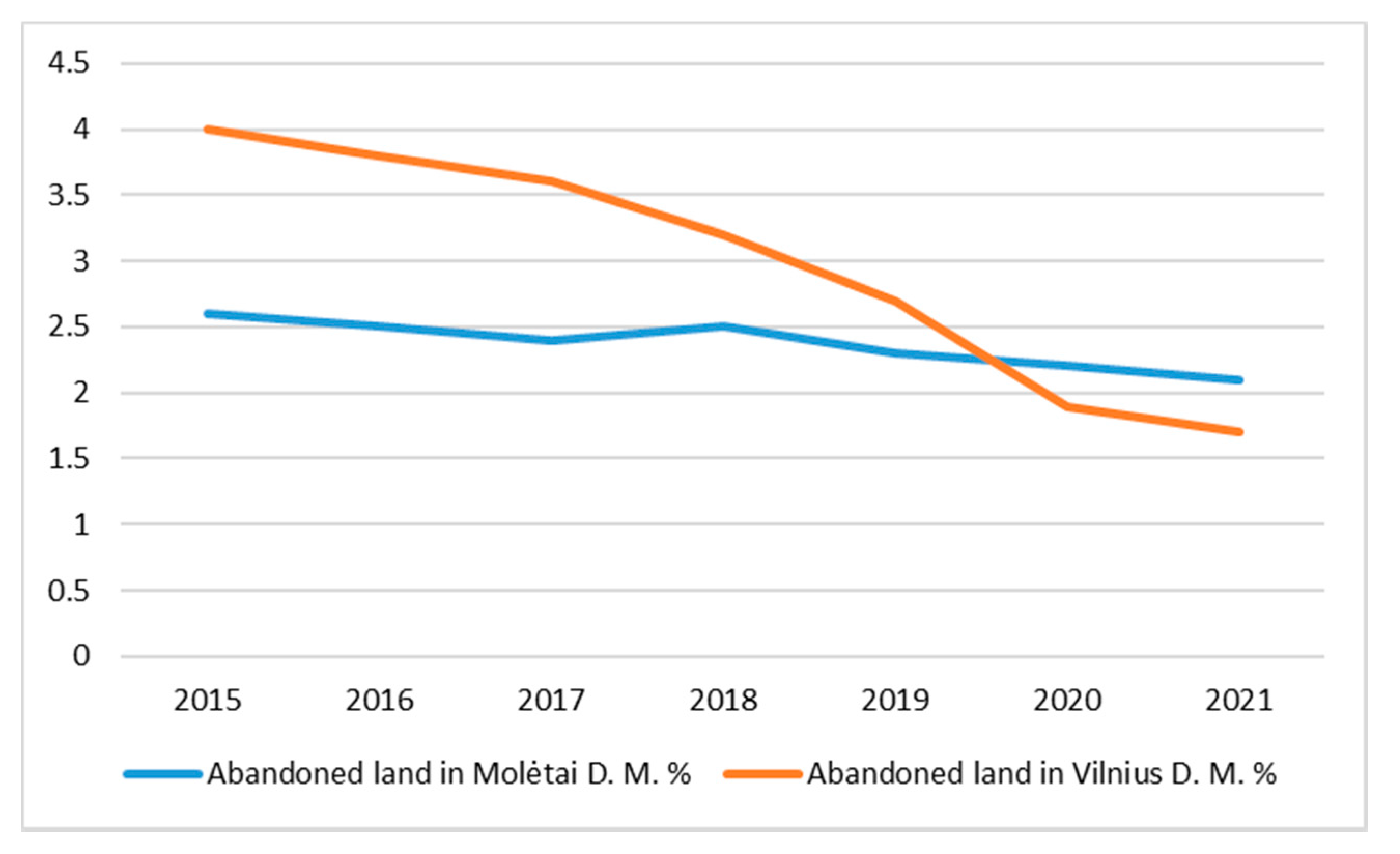
2.1. Study Area

In many regions worldwide, cropland abandonment is growing, which has strong and known environmental and socio-economic consequences [13]. In Lithuania, a sharp decrease in areas of agricultural land was noticed. This decrease can especially be observed from 2016 (Figure 1). Reports of the State Land fund [14] show that areas of agricultural land from 2005 until 2021 have decreased by as much as 2.4%. Agricultural lands that are no longer used for their main purpose are likely to become abandoned and the emergence of such lands can cause a variety of social, economic, and environmental problems.

The area selected for the study, the Moletai district municipality, is located in the eastern part of Lithuania (Figure 2). Changes in agricultural land use in the region have caused various problems such as the abandonment of lands, the spread of particularly aggressive invasive plants in overgrown regions such as H. sosnowskyi (Heracleum sosnowskyi) plants, and so on.

The Moletai district municipality is the district where the largest areas of abandoned land have been recorded in recent years. Although the Vilnius district municipality has been the largest area of abandoned land in Lithuania for a long time, the situation has changed in recent years. Looking at it in the long run (Figure 3), it can be seen that in 2015 the Vilnius district municipality recorded 4% of abandoned agricultural land, although there has been an intense decline of abandoned lands in the region and as of 1 January 2021 only 1.7% of them were recorded.

The 144 km² area of the Moletai district municipality (600 * 600 pixels) was studied in the work. This represents around 10% of the Moletai district municipality, which has a total area of 136,682 km². The aim of the research was to evaluate the seasonality influence for image segmentation results of abandoned lands in selected areas of the Moletai districts municipality.

2.2. Study Data

The following remote sensing and GIS data were used for the procedure of image segmentation and analysis:

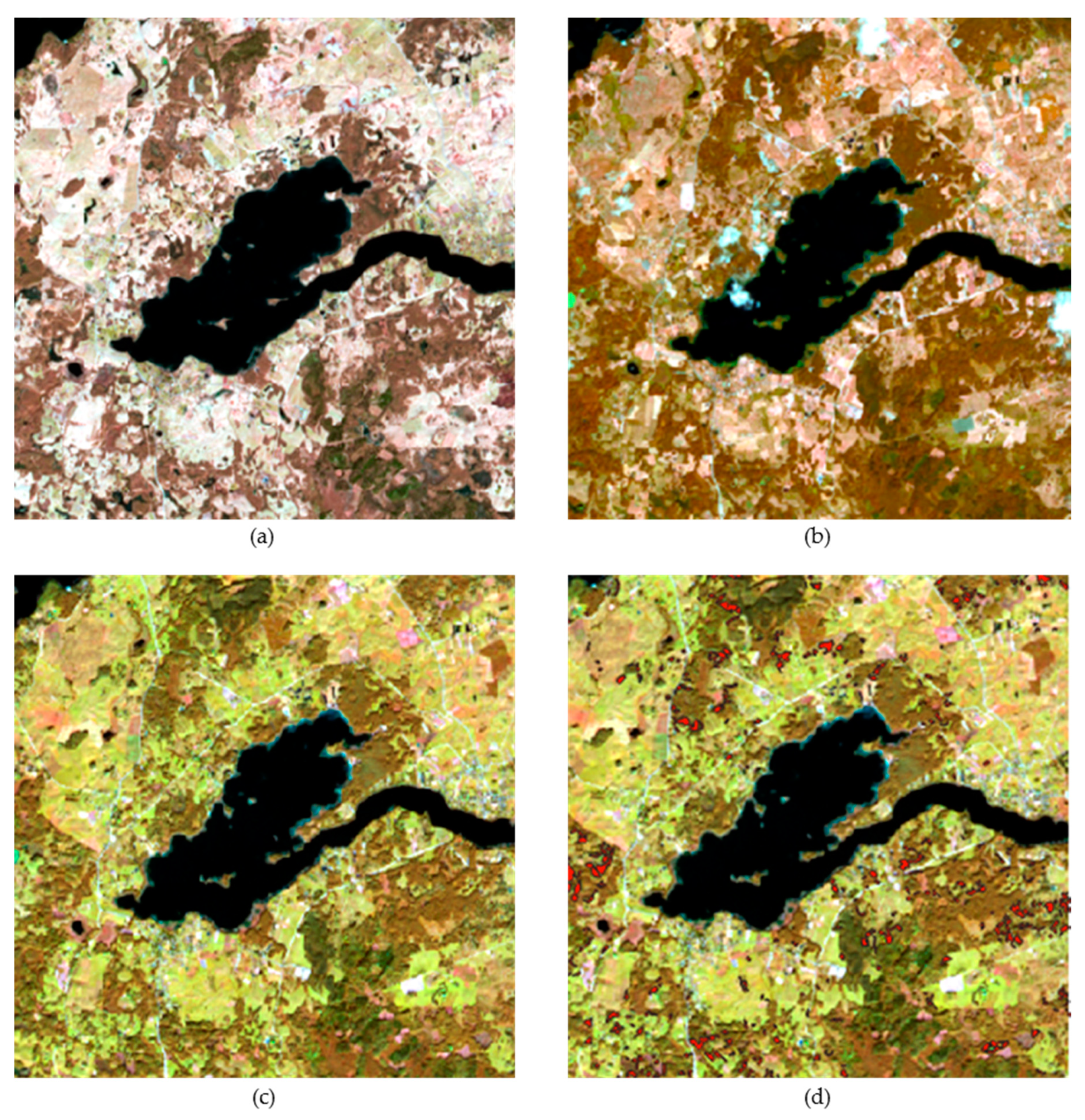
• The multi-spectral Sentinel-2 images:
  • 23 April 2019;
  • 8 July 2019;
  • 10 September 2019.

The images were downloaded from the National Land Service under the Ministry of Agriculture of the Republic of Lithuania. The data was geometrically and atmosphere corrected. A false colour RGB (B8, B4, and B3) combination was used for classification (Figure 4).

2.

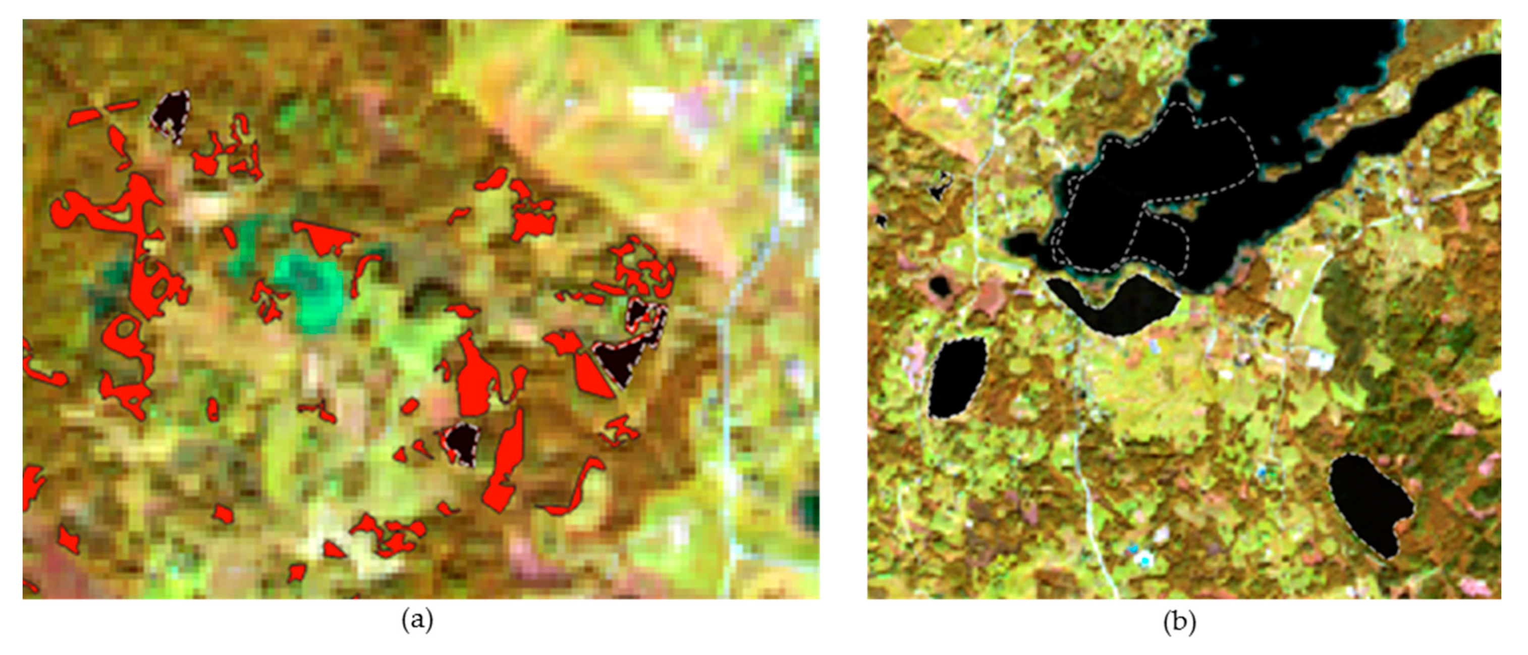
The abandoned land layer was obtained from the open database from the Spatial Information portal in Lithuania [7]. The data are regularly updated.

The false colour imagery (B8, B4, and B3) was displayed in a combination of standard near infra-red, red, and green bands. The use of composites is very popular. It is most commonly used to assess plant density and health, as plants reflect near infrared and green light, while absorbing red light. Since they reflect closer to the infrared than green, plant-covered land appears a darker red colour; indeed, denser plant growth is darker red. Urban land and exposed ground are grey or tan, and water appears blue or black.

2.3. Image Segmentation Methods

Three supervised image segmentation methods were used in this study: SAM; ML; and MD. All methods used the average spectrum of each Region of Interest (ROI).

The supervised image segmentation methods were performed in the QGIS software Semi-automatic Classification Plugin (SCP) tools, as in the study of [16].

2.3.1. Spectral Angle Mapper (SAM)

SAM segmentation was conducted following two work stages [10]:

• The Optimal Spectral Library (OSL) was generated, which preserved the spectral variability present within each ROI. This library could be considered as “optimal” since it contained the spectra that classified all pixels of a certain class correctly, without misclassifying pixels that did not belong to that class. At the same time, for each reference spectrum, a maximum spectral angle distance was calculated, which was used in the second step to avoid misclassifications;
• All image pixels were classified using the reference spectra stored in the OSL, taking into account the calculated maximum spectral angle distance. This meant that each pixel was assigned to the class of the reference spectrum for which the smallest spectral angle value was calculated with the actual pixel spectrum.

In the OSL, the pixel spectra of different vegetation types (vegetation classes Ci) were collected. The SAM and next method calculations used a deterministic similarity measure to compare an unknown pixel spectrum with an OSL library of reference spectra. The smallest spectral angle (θ) could be calculated by the formula given in [10]:

$$\theta =co{s}^{-1}\left(\frac{{\sum }_{i=1}^n{t}_i{r}_i}{\sqrt{{\sum }_{i=1}^n{t}_i{}^2{\sum }_{i=1}^n{r}_i{}^2}}\right)$$

(1)

where n is the number of spectral bands; t is the reflectance of the actual spectrum; and r is the reflectance of the reference spectrum.

Each pixel was assigned to a class according to the lowest spectral angle values. The value was between 0 and π/2. The pixel classification accuracy was calculated by randomly selecting 50% of the ROIs present for a certain class and using them to train the classification (i.e., building the OSL). The remaining 50% of the ROIs of a certain class were used to validate the optimal SAM classification results (i.e., they are classified using the OSL).

One of the most applied strategies for material mapping is the use of similarity measures between vegetation classes Ci. This study made use of a deterministic similarity measure to compare an unknown pixel spectrum with a library OSL of reference spectra. SAM is a common distance metric which compares an unknown pixel spectrum t to the reference spectra for each of the K references and assigns t to the material having the smallest distance:

$$Class\left(t\right)=arg \underset{1\le i\le K}{\min }d\left(t,r_i\right).$$

(2)

The reference spectra of individual pixels can be described as vectors in an n-dimensional space, where n is the number of spectral bands. Each vector has a certain length and direction. The length of the vector represents the brightness of the pixel while the direction represents the spectral feature of the pixel. Variations in illumination mainly affect changes in the length of the vector, while spectral variability between different spectra affects the angle between their corresponding vectors [17].

Scientists have recommended the classification accuracy calculated by randomly selected special vegetation classes’ results and compared with known data (or training layers). In our study, the known data was the abandoned land layer from the open data of the National Land Service under the Ministry of Agriculture of the Republic of Lithuania.

2.3.2. Maximum_Likelihood Image Segmentation Method (ML)

The Maximum_Likelihood image segmentation method is derived from the Bayes theorem [18]. The general processing in ML is as follows:

• The number of land cover types within the study area is determined;
• The training (ROI) pixels for each of the desired classes are chosen using land cover information for the study area. For this purpose, the Jeffries–Matusita (JM) distance can be used to measure the class separability of the chosen training pixels (ROI) [11,12]. The JM distance is a parametric criterion, for which the values range between 0 and 2. The JM considers the distance between the class means and distribution of values from the means. This is achieved by involving the covariance matrices of the classes in the separability measurement [11]. Scientists J. Xie and H.T. Tsui noted that this method can guarantee a good match of the model with the image and avoid assigning high class uncertainties to only these pixels on the ‘‘strongest’’ edges [19]. In the case of the ML per-pixel algorithm, the class to which the pixel is finally assigned is the one with the highest probability. Probabilities of class membership, on which the assignment is based, are usually disregarded so that after classification, no information on the probabilities is available. To overcome the limitations of the classical techniques, such as maximum likelihood classification per-pixel, the “images” are mapped into the likelihood of class labels per sample under the assumption of equal prior probabilities. It is assumed that the normal distribution function will approximate the frequency distributions associated with each of the classes [12]. The maximum probability calculation algorithms described in the Abkar and Sharifi article were also used.

2.3.3. Minimum Distance Segmentation of Image Algorithm

The minimum distance segmentation of image algorithm, Minimum Distance algorithm, calculates the Euclidean distance d(x,y) between the spectral signatures of image pixels and ROI spectral signatures, according to the following equation [16]:

$$d\left(x, y\right)=\sqrt{{\displaystyle \sum }_{i=1}^n{\left(x_i-y_i\right)}^2}$$

(3)

where: x is the spectral signature vector of an image pixel; y is the spectral signature vector of a training area (ROI); and n is the number of image bands.

Therefore, the distance is calculated for every pixel in the image, assigning the class of the spectral signature that is closest, according to the following discriminant function (adapted from [16,20]):

$$x\in C_k\underset{}{\iff }d\left(x,yk\right)<d\left(x,yj\right)\forall k\ne j$$

(4)

where $C_k$ is the land cover class k; $yk$ is the spectral signature of class k; and $yj$ is the spectral signature of class j.

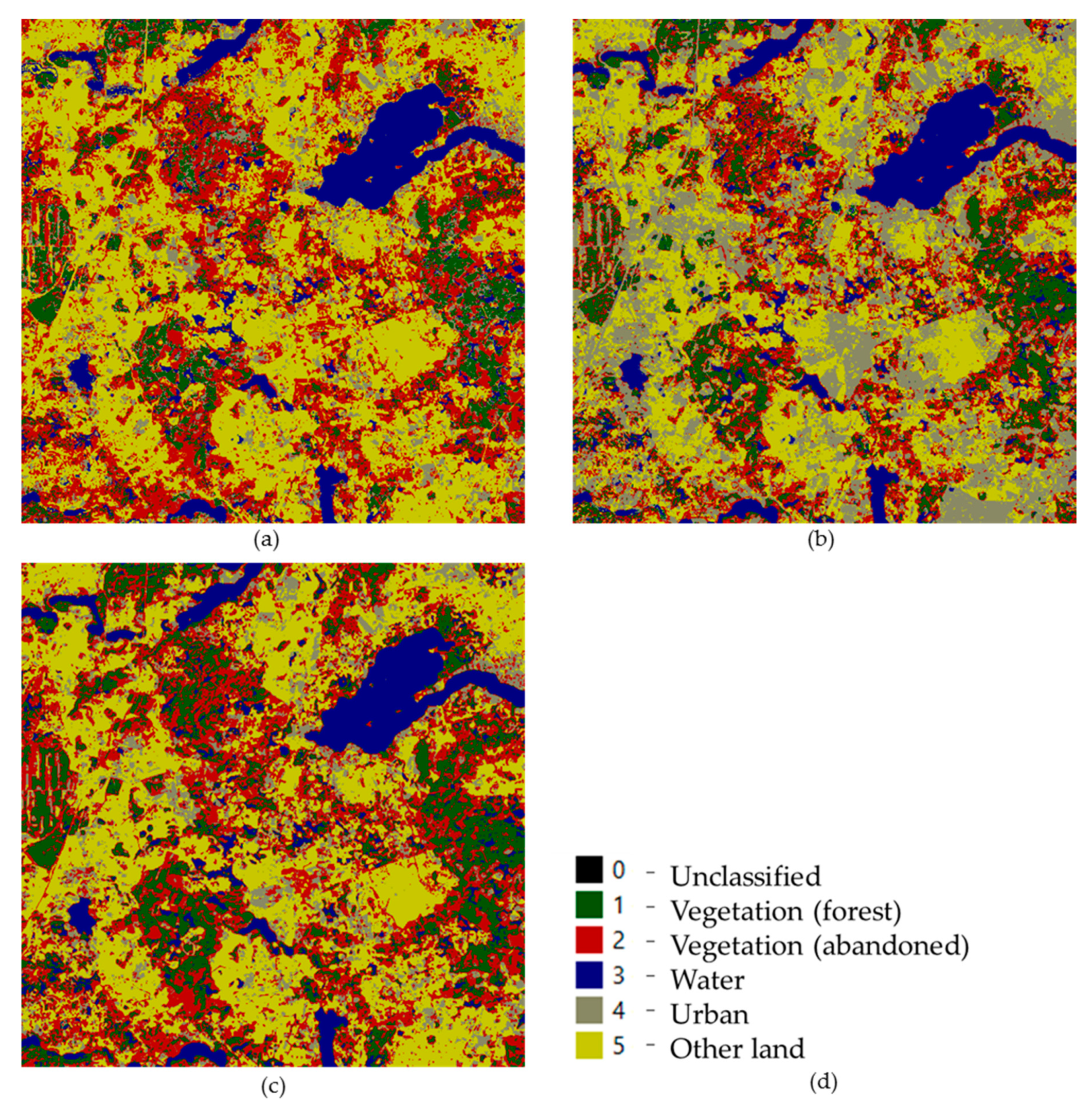
3. Result of Segmentation

In the test area, crop classes were selected: Vegetation (forest and abandoned land), water, urban land, and other land. The abandoned land class ROI was created from an existing layer: The real abandoned land layer (Figure 5a). The following ROIs were created by manually drawing a polygon in the images (Figure 5b).

The next section describes the results for a processed Sentinel-2 image from the months of April, July, and September.

The Sentinel-2 images were subset to the smaller 144-km² area and segmented with the QGIS software Semi-automatic Classification Plugin (SCP). The SCP provides tools for the download, band-processing, pre-processing, and post-processing of images. The band-processing tool has a supervised image classification function with all three used to study segmentation algorithms: Spectral Angle Mapping, Maximum Likelihood, and Minimum Distance. The pre-processing tool could be used to download the Sentinel-2 (Level 2A), which is already atmospherically corrected and could require the conversion of pixel values to a decimal value of reflectance. In this study, we did not use this function because we had our own data. SCP tools of post-processing show reports of pixel classification of different segmentation methods to the cover classes in April, July, and September (

Table 2. Image segmentation results in April.

April
Classes	Colour	Spectral Angle Mapping				Maximum Likelihood				Minimum Distance
		Area, %	Spectral Signature			Area, %	Spectral Signature			Area, %	Spectral Signature
			B3	B4	B8		B3	B4	B8		B3	B4	B8
Vegetation (forest)		9.62	467	724	1593	11.80	443	712	1593	16.28	467	728	1593
Vegetation (abandoned)		29.92	823	1119	2452	21.08	699	995	2211	29.44	823	1119	2452
Water		9.04	214	267	460	9.13	214	267	460	9.14	214	267	460
Urban		9.76	1139	1559	3005	27.84	1192	1548	3017	11.87	1139	1559	3005
Other land		41.66	1169	1552	3567	30.14	1454	1786	3434	33.26	1552	1894	3567

,

Table 3. Results of spectral angle and similarity between classes in April.

Classes	April
	SAM		ML		MD
	θ	S, %	θ	S, %	θ	S, %
Forest–Vegetation (abandoned)	5.69	81	5.61	85	5.69	81
Vegetation (abandoned)–Water	9.63	36	10.12	39	9.63	36
Vegetation (abandoned)–Urban	4.50	84	3.33	80	4.50	84
Vegetation (abandoned)–Other land	3.95	78	4.63	75	3.95	78

,

Table 4. Image segmentation results in July.

July
Classes	Colour	Spectral Angle Mapping				Maximum Likelihood				Minimum Distance
		Area, %	Spectral Signature			Area, %	Spectral Signature			Area, %	Spectral Signature
			B3	B4	B8		B3	B4	B8		B3	B4	B8
Vegetation (forest)		34.31	275	789	1768	0.76	295	632	1003	1.00	324	647	984
Vegetation (abandoned)		10.48	950	1460	2860	1.05	318	709	1315	9.82	302	738	1553
Water		5.14	214	246	222	4.98	211	245	222	5.14	214	246	222
Urban		47.58	669	1241	2541	92.95	602	1145	2343	79.19	561	1120	2357
Other land		2.5	2235	2669	3746	0.26	1480	1874	3488	4.82	1891	2369	3693

,

Table 5. Results of spectral angle and similarity between classes in July.

Classes	July
	SAM		ML		MD
	θ	S, %	θ	S, %	θ	S, %
Forest–Vegetation (abandoned)	20.12	80	2.73	89	6.81	78
Vegetation (abandoned)–Water	26.02	25	-	37	32.74	32
Vegetation (abandoned)–Urban	7.58	92	4.89	78	6.51	86
Vegetation (abandoned)–Other land	12.36	78	24.82	69	24.84	67
Forest–Urban land			5.69	68	5.94	67

,

Table 6. Image segmentation results in September.

September
Classes	Colour	Spectral Angle Mapping				Maximum Likelihood				Minimum Distance
		Area, %	Spectral Signature			Area, %	Spectral Signature			Area, %	Spectral Signature
			B3	B4	B8		B3	B4	B8		B3	B4	B8
Vegetation (forest)		48.30	261	730	1462	8.41	259	604	1276	14.15	233	569	1169
Vegetation (abandoned)		5.20	599	1053	2148	7.14	219	587	1118	35.77	321	790	1612
Water		6.08	134	166	176	6.03	134	166	177	6.23	133	166	178
Urban		39.27	472	1164	2230	78.23	4005	1004	1959	43.44	466	1175	2232
Other land		1.13	1211	1454	2757	0.17	1342	1579	3098	0.41	1462	1729	3227

and

Table 7. Results of spectral angle and similarity between classes in July.

Classes	September
	SAM		ML		MD
	θ	S, %	θ	S, %	θ	S, %
Forest–Vegetation (abandoned)	14.00	87	5.57	94	0.58	84
Vegetation (abandoned)–Water	22.00	24	25.80	33	24.43	26
Vegetation (abandoned)–Urban	23.32	21	5.3	79	2.81	85
Vegetation (abandoned)–Other land	25.85	20.5	32.62	69	28.34	74

). We used the land Macroclass IDs defined in the following classes: Vegetation—forest, vegetation—abandoned, water, urban (build-up), and other lands. The image segmentation results are presented in Section 3.1, Section 3.2 and Section 3.3.

3.1. Segmentation Results of April

The results of the Sentinel-2 (B8, B4, B3) images, segmented with three methods on 23 April 2019 are presented in Figure 6 and in the report (Table 2 and Table 3).

The results of the April image segmentation report (Table 2) were very similar. The area of abandoned lands identified by the SAM method coincided with the results obtained with the MD method. With the ML mode, the obtained area was slightly smaller and had a lower match rate. The most accurately segmented lands were water class land; the compatibility between abandoned lands and water reached 36–39% (Table 3).

Each species has their own chemical composition, which has its own specific spectral signatures. Green is used to discriminate broad vegetation classes and discriminate plant materials. A spectral signature from leaf surfaces is highlighted in the green band (B3) [21]. During spring, there are not that many green plants. Indeed, grasses prevail in such discarded lands and this is why this period is not suitable for distinguishing from satellite imagery. The determined average value of the green (B3) colour spectrum for water-covered areas was the lowest (214), abandoned lands were from 699 to 823, forest areas were from 443 to 467, and urban and other lands differed by a high average spectrum value: 1139 to 1552. The smallest colour mismatch between water and abandoned lands was 36%. (Table 3). Among other segmented land covers and abandoned lands, compatibility was high at 78–85%. This proves once again that it was difficult to single out a segment of a particular plant in an area.

In summary, the images acquired during spring were not suitable for the identification of abandoned lands because shrubs and bushes did not differ much in the colour spectrum from other types of lands.

3.2. Segmentation Results of July

The summer of 2019 was warm and a little cloudy, and therefore, the open access data of Sentinel-2 prepared by the Ministry of Agriculture of the Republic of Lithuania of 8 July 2019 was used to identify vegetation and abandoned lands. The results are presented in Figure 7.

After segmenting the image taken in July, 10.5% consisted of abandoned land areas, 34% of forests, 5% consisted of water bodies, 47% consisted of urbanised areas, and 2.5% consisted of other land were identified using the SAM algorithm (Table 4). The small area of other land indicates that the segmentation was successful because most of the pixels were assigned to some land class. The densest areas of the deserted lands should be inspected on site or compared with the abandoned layer from the Ministry of Agriculture of the Republic of Lithuania to assess their matching percentage. The determined average of the green spectra (950) in the calculations of the SAM algorithm corresponded to the average value determined in the previous studies [3]. The areas of excluded classes calculated by the ML and MD algorithms did not correspond to the real image. In the optical image, the operator easily distinguished between forests, waters, and urban land. As a result of the ML and MD methods, there were no forests and other lands left, and indeed, they were moved to urban land. The mean spectral signature obtained for abandoned lands were wrong.

The similarity between classes corresponds to the spring results (Table 5). Colour compatibility was quite high and only the water body layer (class) could be attributed to reliable information. Vegetation (forest and abandoned land) pixels fell into urban land and additional information on the similarity of forests and urban land showed a 68% compliance. Consequently, the data of abandoned lands have become close to the colour gamut of the built-up area. However, there is still not enough greenness for segmenting the images with the ML or MD algorithm.

3.3. Segmentation Results of September

The image taken in autumn Sentinel-2 (B8, B3, and B4) is characterised by the intensity and brightness of the green colour on 10 September 2019 (Figure 1). The climate is warming and because September was warmer than average, the plants began adapting to the changed natural conditions. There were no yellowing grasses in September yet and the vegetation retained its summer colours. The results of the segmentation of satellite images are shown in Figure 8.

The results are shown in Table 6 and Table 7.

The vegetation (abandoned) land class image segmentation provided good results classifying image pixels with the SAM and ML algorithms. When classifying using the MD algorithm, part of the vegetation (forest) land class was moved to the vegetation (abandoned) land class, resulting in the area of abandoned lands increasing by as much as 5 times (from 5% to 35.77%) and the reliability of the data decreased. This was also reflected in the colour compatibility results (Table 7). The compatibility between Forest and Abandoned lands was highest and ranged from 87% to 94%. However, according to the ROI sample, the compatibility of abandoned lands with water, urban land, and other lands was only 21–26%, which was the best option for image segmentation in spring, summer, and autumn.

Summarising the segmentation results of the September image, it can be stated that this was the most suitable image for the identification of abandoned lands, if the September weather corresponded to the warm summer weather (as it was in 2019). The calculated mean spectral signature of abandoned land 599 (B3) (SAM) is recommended to be used automatically when segmenting pictures taken during September. The value 219 (B3) computed with the ML algorithm was close to the mean spectral signature of the forest layer, although data can be unreliable during automatic segmentation.

3.4. Segmentation Results Analysis

Studies have found that the most appropriate time to segment abandoned lands is during September with the SAM and ML algorithms. During this period the intensity of the green colour is the highest and the colour brightness of abandoned lands differs in colour intensity with other lands (Figure 9).

The mean spectral signature of water is 134, forest—261, urban lands—472, abandoned lands—599, and other lands—1200. Mean spectral signature values vary depending on seasons. Previous studies have found and it has been confirmed in this study that the mean spectral signature of abandoned lands is 950 in summer and 699–823 in spring. This parameter needs to be known to perform automatic abandoned land segmentation.

4. Conclusions and Discussion

This paper provides the results of multispectral Sentinel-2A (falsecolour RGB (B8, B4, B3) combination) data for land cover classifications during different seasons. The April, July, and September images were segmented with three supervised segmentation methods: Spectral Angle Mapping, Maximum Likelihood, and Minimum Distance. This study showed that seasonality and the segmentation algorithm had an effect on the results of image segmentation.

Finding an optimal time and algorithm for the data acquisition is therefore important in all mapping applications based on remotely sensed datasets [1,22]. When images from different seasons are acquired, changes caused by phenological differences can result in the mapping of a change in condition, rather than a change in land cover or land use [22,23]. Otherwise, authors have recommended combining methods with different satellites systems.

Plants in early spring have little green colour, and in summer, autumn green colour intensity is affected by the climate. If the autumn is warm, as it recently has been in the territory of Lithuania, then this is the most appropriate time to identify green plants. This is evident in the colour gamma, contrast, and data structure of the images (Figure 4). In the study area, the abandoned lands identified with the SAM algorithm coincided with the results of the MD and ML methods during springtime. The vegetation, especially on abandoned lands, did not differ from the urbanised and other lands. After pixel classification, even forest land fell into the layer of “other land”. The spring images could be segmented automatically and later had their identified segments assigned to a particular land class. However, this process would take a long time without such data.

The SAM algorithm was found to be suitable for segmenting the images taken during the summer only. Segmentation by other MD and ML algorithms moved vegetation (forest and abandoned lands) data to an urbanised area, most likely due to the spectral similarity of the pixels. The spectral angle algorithms constrained active contour models, combining the level set functions that were, in general, less sensitive to the initial contour curve placement and more robust in complex images [24]. The Active Contour Model (ACM) was used to construct an initial contour for an “energy” in the ROI, and then made the initial contour evolve toward the target boundary under the principle of minimum energy by computing the optimal solution of the energy functional.

The September image was the most suitable image for identifying vegetated (forest, abandoned) lands, water, urban, and other lands. The image segmentation algorithm SAM and ML both worked. According to the physical characteristics of remote sensing, the reflection (or absorption) spectrum of the object could reflect differences in the composition and structure of objects. As a result, the shape of the spectral curve could be used to distinguish an object [24]. The spectral similarity between lands was 20–24%. The result showed that autumn images segmented with the SAM algorithm were the most accurate. To assess their reliability and accuracy the authors recommend comparing the results with known information and subtracting the differences to calculate the Kappa coefficient. In our case, the formats of the results and existing data were not suitable for this analysis. Scientist Cohen proposed using a Kappa coefficient to assess accuracy in 1960 [25,26]. However, a very accurate classification could be associated with a very wide range of Kappa values [26].

5. Recommendation

The authors of this study recommend taking out the abandoned land areas that are in the forest area from the segmentation results and checking the final results using field measurements. This is planned to be done in future.

Based on these research results, the authors recommend segmenting abandoned lands during September with the Spectral Angle Mapping (SAM) algorithm in the multispectral Sentinel-2A (falsecolour RGB (B8, B4, and B3) combination) data. However, it is necessary to take into account the current air temperature, which influences the photosynthesis of plants on which depends the mean spectral signature value.

References

1. Karila, K.; Matikainen, L.; Litkey, P.; Hyyppa, J.; Puttonen, E. The effect of seasonal variation on automated land cover mapping from multispectral airborne laser scanning data. Int. J. Remote Sens. 2018, 40. [Google Scholar] [CrossRef] [Green Version]
2. Sheeren, D.; Fauvel, O.M.; Josipović, V.; Lopes, M.; Planque, C.; Willm, J.; Dejoux, J.F. Tree Species Classification in Temperate Forests Using Formosat-2 Satellite Image Time Series. Remote Sens. 2016, 8, 734. [Google Scholar] [CrossRef] [Green Version]
3. Sužiedelytė Visockienė, J.; Tumelienė, E.; Malienė, V. Identification of Heracleum sosnowskyi-invaded land using earth remote sensing data. Sustainability 2020, 12, 759, ISSN 2071-1050. [Google Scholar] [CrossRef] [Green Version]
4. Song, W. Mapping Cropland Abandonment in Mountainous Areas Using an Annual Land-Use Trajectory Approach. Sustainability 2019, 11, 5951. [Google Scholar] [CrossRef] [Green Version]
5. Order of the Government of the Republic of Lithuania. On Establishment of Lithuanian Geodetic Coordinate System; Dėl Lietuvos Geodezinių Koordinačių Sistemos Įvedimo; No. 936; Lietuvos Respublikos Vyriausybės Nutarimas: Vilnius, Lithuania, 1994. (In Lithuanian) [Google Scholar]
6. Radiometric Resolutions. 2021. Available online: https://sentinels.copernicus.eu/web/sentinel/user-guides/sentinel-2-msi/resolutions/radiometric (accessed on 2 April 2021).
7. Spatial Information Portal of Lithuania. 2021. Available online: www.geoportal.lt (accessed on 2 April 2021).
8. Unsalan and Boyer. Multispectral Satellite Image Understanding. 2011. Available online: https://www.researchgate.net/publication/321515169 (accessed on 25 April 2021). [CrossRef] [Green Version]
9. Rosenberger, C.; Chabrier, S.; Laurent, H.; Emile, B. Unsupervised and Supervised Image Segmentation Evaluation. 2006. Available online: https://www.researchgate.net/publication/257365161 (accessed on 5 May 2021). [CrossRef]
10. Bertels, L.; Deronde, B.; Kempeneers, P.; Debruyn, W.; Provoost, S. Optimized Spectral Angle Mapper classification of spatially heterogeneous dynamic dune vegetation, a case study along the Belgian coastline. In Proceedings of the 9th International Symposium on Physical Measurements and Signatures in Remote Sensing (ISPMSRS), Beijing, China, 17–19 October 2005. [Google Scholar]
11. Dobbor, M.; Hower, S.; Shokr, M.; Yackel, J.J. Howell the Jeffries–Matusita distance for the case of complex Wishart distribution as a separability criterion for fully polarimetric SAR data. Int. J. Remote Sens. 2014, 35, 6859–6873. [Google Scholar]
12. Abkar, A.A.; Sharifi, M.A. Likelihood-Based Image Segmentation and Classification: Concepts and Applications. In Proceedings of the ISPRS 2000 Congress: Geoinformation for All, Amsterdam, The Netherlands, 16–23 July 2000; Volume XXXIII, pp. 9–16. [Google Scholar]
13. Low, F.; Fliemann, E.; Abdullaev, I.; Conrad, C.; Lamers, J.P.A. Mapping abandoned agricultural land in Kyzyl-Orda, Kazakhstan using satellite remote sensing. Appl. Geogr. 2015, 62, 377–390. [Google Scholar] [CrossRef]
14. National Land Service under the Ministry of Agriculture. Reports of State Land Fund. 2005–2021; National Land Service under the Ministry of Agriculture: Vilnius, Lithuania, 2005–2021. [Google Scholar]
15. Land Information System. Available online: https://zis.lt/ (accessed on 3 June 2021).
16. Congedo, L. Semi-Automatic Classification Plugin for QGIS; Project Title: Adapting to Climate Change in Coastal Dar es Salaam, Ref. EC Grant Contract No. 2013. 2010/254-773; Sapienza University of Rome: Rome, Italy, 2013. [Google Scholar]
17. Kruse, F.A.; Lefkoff, A.B.; Boardman, J.W.; Heidebrecht, K.B.; Shapiro, A.T.; Barloon, P.J.; Goetz, A.F.H. The spectral image processing system (SIPS)—interactive visualization and analysis of imaging spectrometer data. Remote Sens. Environ. 1993, 44, 145–163. [Google Scholar] [CrossRef]
18. Ahmad, A. Analysis of maximum likelihood classification on multispectral data. Appl. Mathemat. Sci. 2012, 6, 6425–6436. [Google Scholar]
19. Xie, J.; Tsui, H.T. Image segmentation based on maximum-likelihood estimation and optimum entropy-distribution (MLE–OED). Pattern Recognit. Lett. 2004, 25, 1133–1141. [Google Scholar] [CrossRef]
20. Richards, J.A.; Jia, X. Remote Sensing Digital Image Analysis. An Introduction; Springer: Berlin/Heidelberg, Germany, 2006; Available online: https://www.springer.com/gp/book/9783642300615#otherversion=9783642300622 (accessed on 5 May 2021).
21. GIS Geography, Spectral Signature. 2021. Available online: https://gisgeography.com/spectral-signature/ (accessed on 7 April 2021).
22. Silveira, E.M.O.; Bueno, I.T.; Acerbi-Junior, F.W.; Mello, J.M.; Scolforo, J.R.S.; Wulder, M.A. Using Spatial Features to Reduce the Impact of Seasonality for Detecting Tropical Forest Changes from Landsat Time Series. Remote Sens. 2018, 10, 808. [Google Scholar] [CrossRef] [Green Version]
23. Lu, M.; Chen, J.; Tang, H.; Rao, Y.; Yang, P.; Wu, W. Land cover change detection by integrating object-based data blending model of Landsat and MODIS. Remote Sens. Environ. 2016, 184, 374–386. [Google Scholar] [CrossRef]
24. Wang, X.; Li, Z.; Zhou, X.; Tao, J. Segmentation model for hyperspectral remote sensing images based on spectral angle constrained active contour. Multimed. Tools Appl. 2019, 78, 10141–10155. [Google Scholar] [CrossRef]
25. Cohen, J. A Coefficient of Agreement for Nominal Scales. Educ. Psychol. Meas. 1960, 20, 37–46. [Google Scholar] [CrossRef]
26. Foody, G.M. Explaining the unsuitability of the kappa coefficient in the assessment and comparison of the accuracy of thematic maps obtained by image classification. Remote Sens. Environ. 2020, 239, 111630. [Google Scholar] [CrossRef]
Figure 1. Area of agricultural land changes from 2005 to 2021 (the data were determined before 1 January of the specified year) [14].
Sustainability 13 06941 g001
Figure 2. Study area in the Moletai district municipality [15].
Sustainability 13 06941 g002
Figure 3. Dynamic of abandoned agricultural land areas (%) in the Vilnius and Moletai district municipalities from 2015 to 2021, evaluating the area of each municipality (the data were determined before 1 January of the specified year).
Sustainability 13 06941 g003
Figure 4. The fragment of false colour RGB (B8, B4, B3) images: (a) 23 April 2019; (b) 8 July 2019; (c) 10 September 2019; and (d) 10 September 2019 and abandoned land layer (area in red).
Sustainability 13 06941 g004
Figure 5. ROI in the images: (a) The abandoned land (ROI in black), and (b) water, forest, and other land (black).
Sustainability 13 06941 g005
Figure 6. April’s Sentinel-2 image segmentation results: (a) Spectral Angle Mapping segmentation; (b) Maximum Likelihood segmentation; (c) Minimum Distance segmentation; and (d) Land classes.
Sustainability 13 06941 g006
Figure 7. July’s Sentinel-2 image segmentation results: (a) Spectral Angle Mapping segmentation; (b) Maximum Likelihood segmentation; (c) Minimum Distance segmentation; and (d) Land classes.
Sustainability 13 06941 g007
Figure 8. Sentinel-2 image segmentation results for September: (a) Spectral Angle Mapping segmentation; (b) Maximum Likelihood segmentation; (c) Minimum Distance segmentation; and (d) Land classes.
Sustainability 13 06941 g008
Figure 9. Mean spectral signature value of land classes in the bands: Green—vegetation (forest); red—vegetation (abandoned); blue—water; grey—urban; and khaki—other land.
Sustainability 13 06941 g009