Article

Carbon Cycling in Mangrove Ecosystem of Western Bay of Bengal (India)

by
Kakoli Banerjee
1,*,
Abhijit Mitra
2 and
Sebastián Villasante
3
1
Department of Biodiversity & Conservation of Natural Resources, Central University of Odisha, Landiguda, Koraput 764021, India
2
Department of Marine Science, University of Calcutta, 35 B.C. Road, Kolkata 700019, India
3
Department of Applied Economics, University of Santiago de Compostela, 15705 A Coruña, Spain
*
Author to whom correspondence should be addressed.
Sustainability 2021, 13(12), 6740; https://doi.org/10.3390/su13126740
Submission received: 9 May 2021 / Revised: 8 June 2021 / Accepted: 9 June 2021 / Published: 15 June 2021

Abstract

:
Carbon cycling in the mangrove ecosystem is one of the important processes determining the potential of coastal vegetation (mangroves), sediment, and adjoining waters to carbon absorption. This paper investigates the carbon storage capacity of five dominant mangrove species (Avicenia marina, Avicenia officinalis, Excoecaria agallocha, Rhizophora mucronata, and Xylocarpous granatum) on the east coast of the Indian mangrove along with the role they play in the carbon cycling phenomenon. Soil and water parameters were analyzed simultaneously with Above Ground Biomass (AGB) and Above Ground Carbon (AGC) values for 10 selected stations along. The total carbon (TC) calculated from the study area varied from 51.35 ± 6.77 to 322.47 ± 110.79 tons per hectare with a mean total carbon of 117.89 ± 28.90 and 432.64 ± 106.05 tons of carbon dioxide equivalent (CO2e). The alarm of the Intergovernmental Panel on Climate Change for reducing carbon emissions has been addressed by calculating the amount of carbon stored in biotic (mangroves) and abiotic (soil and water) compartments. This paper focuses on the technical investigations on the factors that control the carbon cycling process in mangroves. This blue carbon will help policymakers to develop a sustainable relationship between marine resource management and coastal inhabitants so that carbon trading markets can be developed, and the ecosystem is balanced.

1. Introduction

Mangrove forests make a versatile depository for low-cost climate mitigation scenarios owing to their special adaptation [1]. Mangroves are unique halophytic vegetation (tree or shrub) that grows in tropical and subtropical regions, >1 m in elevation above MSL [2]. Considering the world’s forest status, mangroves constitute about 0.7% and 0.1% of tropical forest and total forest area respectively [3] with America 11%, Africa 20%, and Asia 42%, respectively. In the case of tropical mangroves Sundarbans, Mekong Delta, Madagascar, Papua New Guinea, and the Philippines occupy the biggest patches. The maximum number of the true mangrove species are confined to the Southeast Asian region [4,5]. Previous studies have reported globally for the potential carbon sequestration property of mangroves to be 1.8 × 10⁸ tCyr−1 and that of soil carbon to be 1.023 × 10⁹ tCm−2 [3], considering the depth of 3 m for SE Asia.
India is a sub-continental country of south Asia, with a total coastline of 7516.6 km, with the Bay of Bengal, Indian Ocean, and the Arabian Sea respectively on three sides of the country including Andaman-Nicobar and Lakshadweep islands. The mangroves are distributed in the nine major States including two union territories Puducherry, Daman and Diu, and Andaman–Nicobar Islands of India [6,7]. The mangrove forest of Bhitarkanika Wildlife Sanctuary, regarded as the second largest coastal dense forest after Sunderbans, has an area of 197 km2 out of 4921 km2 of the total mangrove forests in India [7]. Studies on biomass and carbon in Mahanadi Delta of Odisha has documented overall mean carbon stock of 147.0 ± 8.1 tCha–1 (vegetation 89.4 ± 7.6 and soil 57.6 ± 3.2 tCha–1 up to a depth of 30 cm), in which there is a natural stand of 143.4 ± 8.2 tCha–1 (vegetation 89 ± 8.9 and soil 54.3 ± 3 tCha–1) and plantation of 151.5 ± 7.9 tCha–1 (vegetation 90.6 ± 16.2 and 60.9 ± 5.6 tCha–1) [8]. Banerjee et al. [9] reported the various physical, biological and anthropogenic factors influencing the soil organic carbon. Sahoo and Dhal [10] reported the organic carbon in the sediment was found to be 1.7, 10.16, and 19.20 mg·g–1 in the Bhitarkanika mangrove ecosystem respectively.
Carbon cycling refers to the absorption of carbon dioxide from the atmosphere and conversion to carbohydrates by salt marshes, mangroves, seagrasses, phytoplankton, algae, micro-organisms, and organisms with calcium carbonate covering. During outwelling, this carbon is washed off to the sea and through transformation, carbon fluxes are established (Figure 1). Mangroves and their associated vegetation help in trapping the upwelled waters adding nutrients to the sediment and to the adjoining waters [11]. Coastal sediments in the mangrove ecosystem account for 50% of carbon storage thereby playing a major role in carbon biogeochemical cycling [12].
In recent years, blue carbon (which encompasses the carbon stored in mangroves, salt marsh grasses, seagrasses, coastal sediments, and the adjoining water bodies) research has gained momentum internationally partially in science and partially in policy. International organizations like Conservation International (CI), International Union for Conservation of Nature (IUCN), Intergovernmental Oceanographic Commission (IOC), and United Nations Educational Scientific and Cultural Organization (UNESCO) have also come up with various projects on quantification of blue carbon in different coastal ecosystems.
Mangrove carbon cycling is linked to soil carbon, stored carbon in biomass, atmosphere, and the adjacent mangrove waters which are large surface pools of dissolved inorganic matter (DIC). The present paper focuses on the carbon cycling in the bottom-top approach from sediment to seawater, mangroves, and then to the atmosphere by calculating the amount of carbon dioxide being absorbed and stored by the mangroves along with its sediment and adjoining seawater in the western Bay of Bengal. The study also suggests the use of Payment for Ecosystem Services (PES) policies not only for mangrove biomass but also for sediment carbon.

2. Materials and Methods
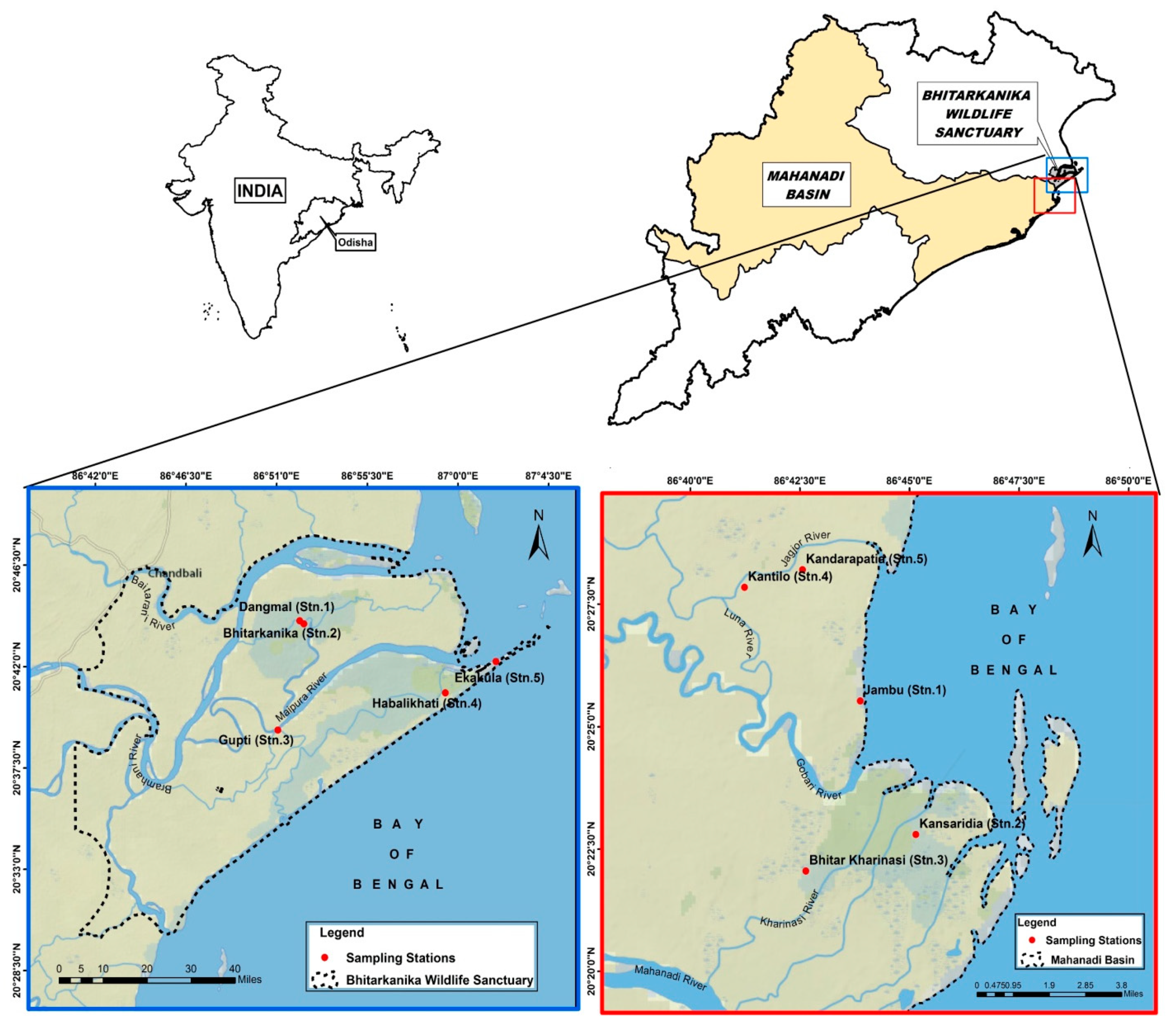
2.1. Study Area

The western Bay of Bengal comprises two major mangrove chunks viz. Bhitarkanika Wildlife Sanctuary and the southern part of it, the Mahanadi mangroves. The two mangrove chunks are noted for their own characteristics, the former being a reserve forest area with dense mangroves and the other an anthropogenically disturbed zone with moderately dense vegetation. Both the areas are located in the Kendrapara district of Odisha and form the estuarine complex of River Mahanadi with the Bay of Bengal. The Bhitarkanika Wildlife Sanctuary located between the coordinates 20°40′ to 20°48′ N latitude and 86°45′ to 87°50′ E longitude covers an area of 0.0672 ha where 5 sampling sites (Stns. 1–5) namely Dangmal, Bhitarkanika, Gupti, Habalikhati, and Ekakula were selected. The Mahanadi estuarine complex covering 6651 ha is located between 20°18′ to 20°32′ N latitude and 86°41′ to 86°48′ E longitudes in Odisha where 5 stations (Stns. 1–5) were selected in the tidal creeks namely Jambu, Kansaridia, Kandarapatia, Kantilo, and Bhitar Kharnasi, respectively. The region experiences a hot and humid climate and is regularly flooded with tidal waters from the Bay of Bengal (Table 1 and Figure 2).

2.2. Estimation of above Ground Biomass and above Ground Carbon

Around 15 sampling plots in each sampling station with 10 m × 10 m quadrats were laid seasonally and only live trees with a diameter at breast height (DBH) ≥ 5 cm were recorded for examining biomass and carbon in mixed stands focusing on the dominant species viz. Avicennia marina, Avicennia officinalis, Excoecaria agallocha, Rhizophora mucronata and Xylocarpus granatum as per standard formulae [13]. The plots were selected in such a way that all species were presented enough. Seasonal sampling (premonsoon, monsoon, and postmonsoon) during low tide has been carried out over a period of 2 years. Bosch Range Finder (DLE 40 professional) was used to determine the total height of the tree. The stem volume was calculated as: V = πr2H, where, V = volume of the plant, π = 3.14, r = radius of the plant H = height of the plant. Wood density (g/cm3) of dry wood was estimated by taking a stem core of 1 cm3 which was further converted into stem biomass as per the expression: B = WD × V, where, B = Biomass, WD = Wood density, and V = Volume of the stem. Branch groups were selected by branch diameter and then branch biomass was estimated using the equation:
B db = n 1 bw 1 + n 2 bw 2 + n 3 bw 3 =   nibwi
where Bdb is the dry branch biomass per tree, ni the number of branches in the ith branch group, bwi the average weight of branches in the ith group, and i = 1, 2, 3, n are the branch groups. The leaf biomass per tree was calculated by multiplying the average biomass of the leaves per branch with the total number of branches in that tree. Finally, the dry leaf biomass of the selected mangrove species (for each plot) was recorded as per the expression:
Ldb = n1Lw1N1 + n2Lw2N2 +...niLwiNi
where Ldb is the dry leaf biomass of selected mangrove species per stations, n1 ... ni are the number of branches of each tree of three dominant species, Lw1 ... Lwi are the average dry weight of leaves removed from the branches, and N1 ... Ni are the number of trees per species in the stations.
Carbon was analyzed by a Vario MACRO elementar CHN analyzer. CO2 equivalent was calculated for each species by multiplying factor 3.67 (ratio of molar masses) with AGC to express the value in tons of CO2. Carbon sequestration rate (CSR) is calculated by dividing the total carbon accumulated over the specific time period (at the beginning and at the end of our study period). Carbon fluxes were calculated between annual mean storages in both the study sites taking the ratio between carbon storage between atmosphere to ocean and atmosphere to land.

2.3. Analysis of Soil Organic Carbon (SOC)

The Walkley and Black [14] protocol was used to determine SOC. Soil samples (15 in number at each sampling station) were collected from 1 to 5 cm depth. These samples were cleaned leaving the underground roots, twigs, and barks. These soils along with blanks were titrated with Mohr salt solution and the volume of K2Cr2O7 consumed to oxidize organic carbon was calculated from the difference. Percentage of carbon was expressed as C (%) = 3.951/g (1-S/B), where g = weight in grams of sample, S = volume of Mohr’s salt solution concentration made by sample, B = volume of Mohr’s salt solution concentration consumed by a blank.

2.4. Analysis of Dissolved Inorganic Carbon (DIC)

DIC was analyzed in water samples through potentiometric titration as per the method outlined by Edmond [15] with an accuracy level of ±0.3 µmol/L. Total dissolved inorganic carbon (DIC) was measured on board by using a technique based on the potentiometric method with a closed-cell described by Goyet et al. [16]. The calculation of the equivalent point is estimated using a non-linear regression method of DOE [17]. During the estimation, we used the Certified Referenced Material (CRM, Batch#28). Based on CRM analyses and replicates, the analysis of surface water samples, the precision of DIC was estimated to be around 2 µmol/L, which is the precision achieved during most of the analyses.

2.5. Statistical Analyses

About 15 samples of soil and 50 samples for mangrove species were collected from each sampling station to maintain homogeneity of observations. After collection, species-wise segregations were done, processed, and then subsequently analyzed for biomass and carbon. Mean and standard deviations were calculated for the data. In order to understand the spatial and temporal variation of the selected parameters, MANOVA was computed using IBM SPSS Statistics-21 software, keeping physico-chemical parameters, AGB and AGC (per species) as dependent variables and stations and seasons as fixed factors.

3. Results and Discussion

The present research has tried to document the carbon storage capacity of adjacent seawater, soil, and selected mangroves in the study area and, in turn, calculating carbon dioxide equivalent (CO2e) for understanding the amount of CO2 that is being absorbed from the atmosphere, thereby trying to establish the carbon cycle.

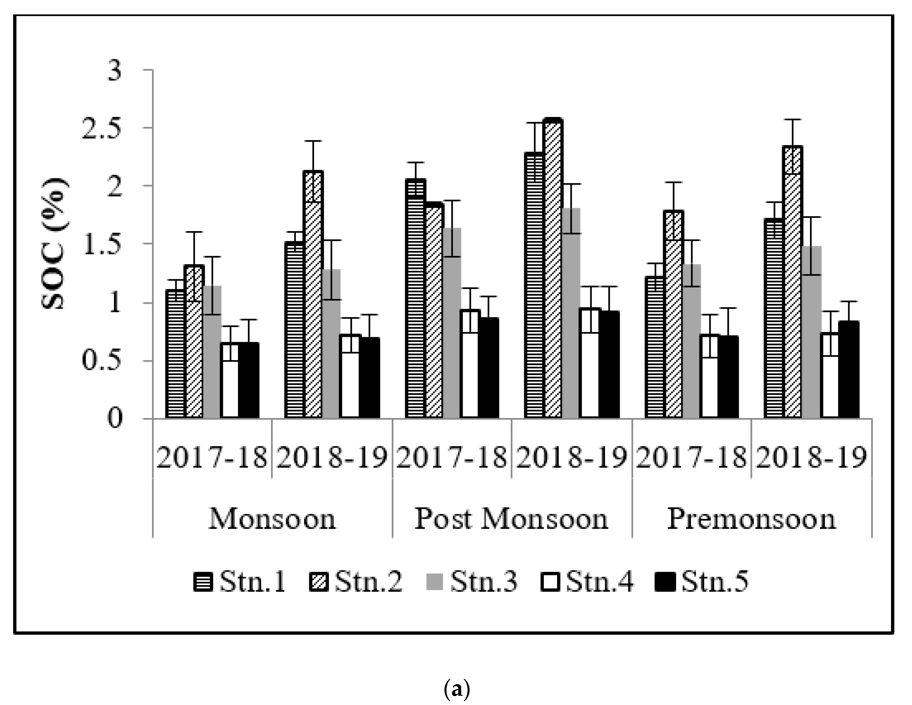
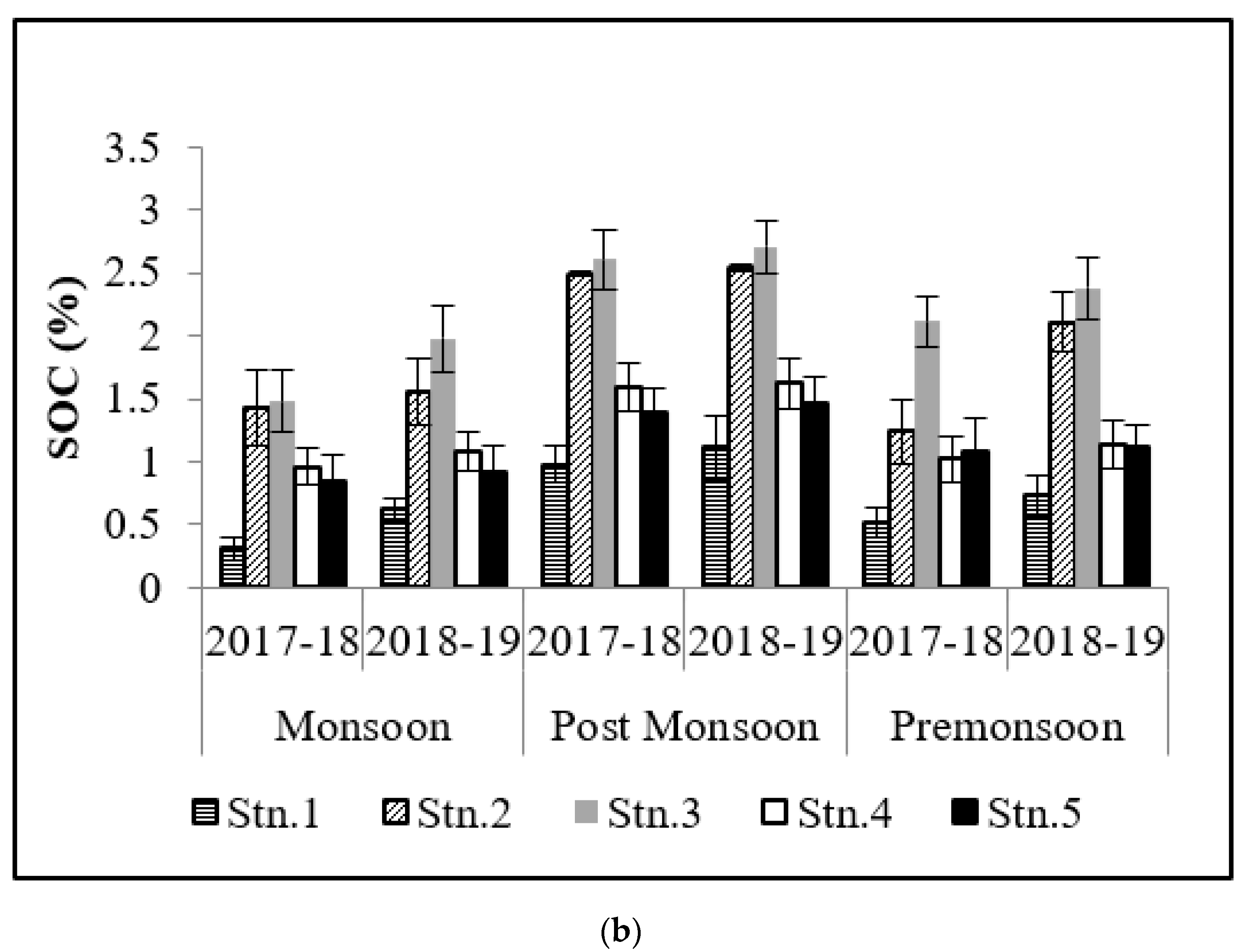
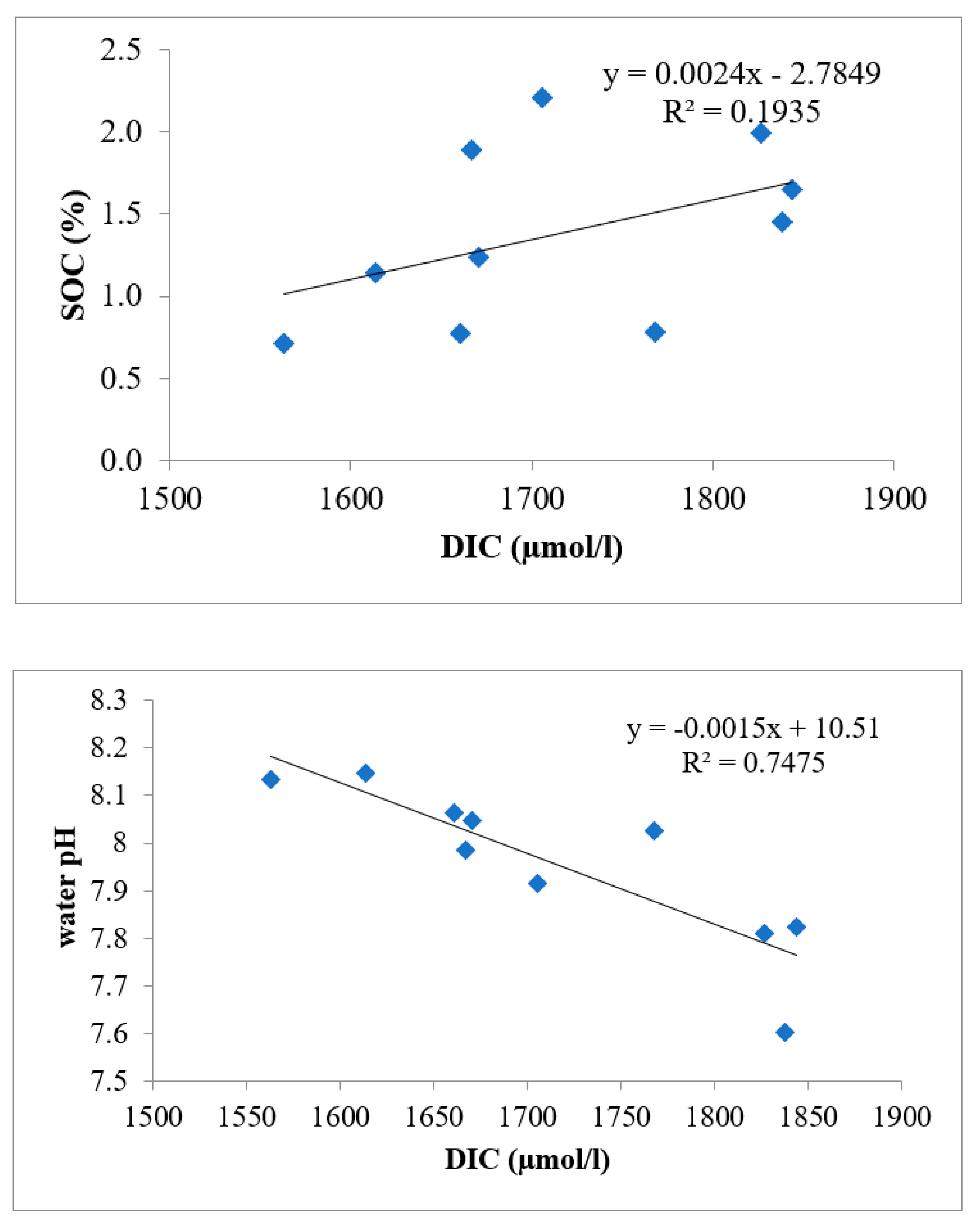
3.1. Soil Organic Carbon (SOC)

SOC contributes significantly to the carbon cycle as it plays a major role in the mineralization of hydrogen and carbon through microbes and also enriches the adjoining waters during outwelling. Hence, the density of vegetation and climate of the area both have significant roles to play [18]. The highest values of SOC in post-monsoon (2.71 ± 0.03%) is a reflection of the stored carbon after the monsoon precipitation (0.31 ± 0.04%) from the adjoining landmass (Figure 3). Over the last two years (2017–2018 and 2018–2019), it has been observed that SOC values are comparatively higher at Stns.1, 2, and 3 at Bhitarkanika and Stn.2 and 3 at Mahanadi mangrove ecosystem owing to the fact that these stations are areas with dense mangrove patches. ANOVA results have shown significant spatial and temporal variations that have also been reported by Reddy and Hariharan [19]. SOC values were lower in monsoon and higher in post-monsoon which may be attributed to the more microbial degradation (owing to the moist condition) of accumulated inorganic matter, which favors high organic matter in sediments [20]. The present study has indicated that high saline soils have a low potential for carbon storage which may be due to the poor growth of mangroves [21]. The dependence of carbon storage potential on soil quality has also been stated by Canadell et al. [22].

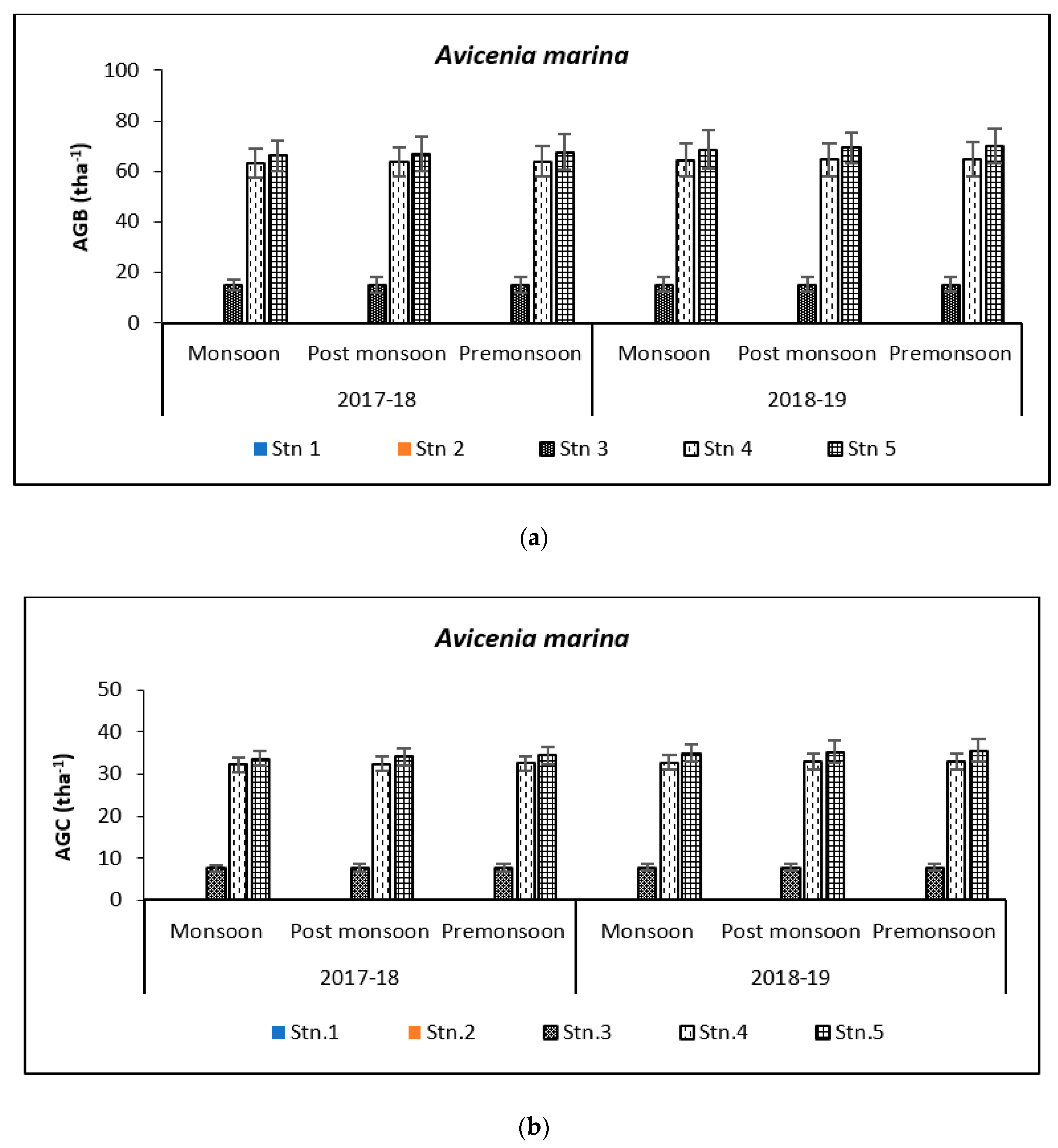
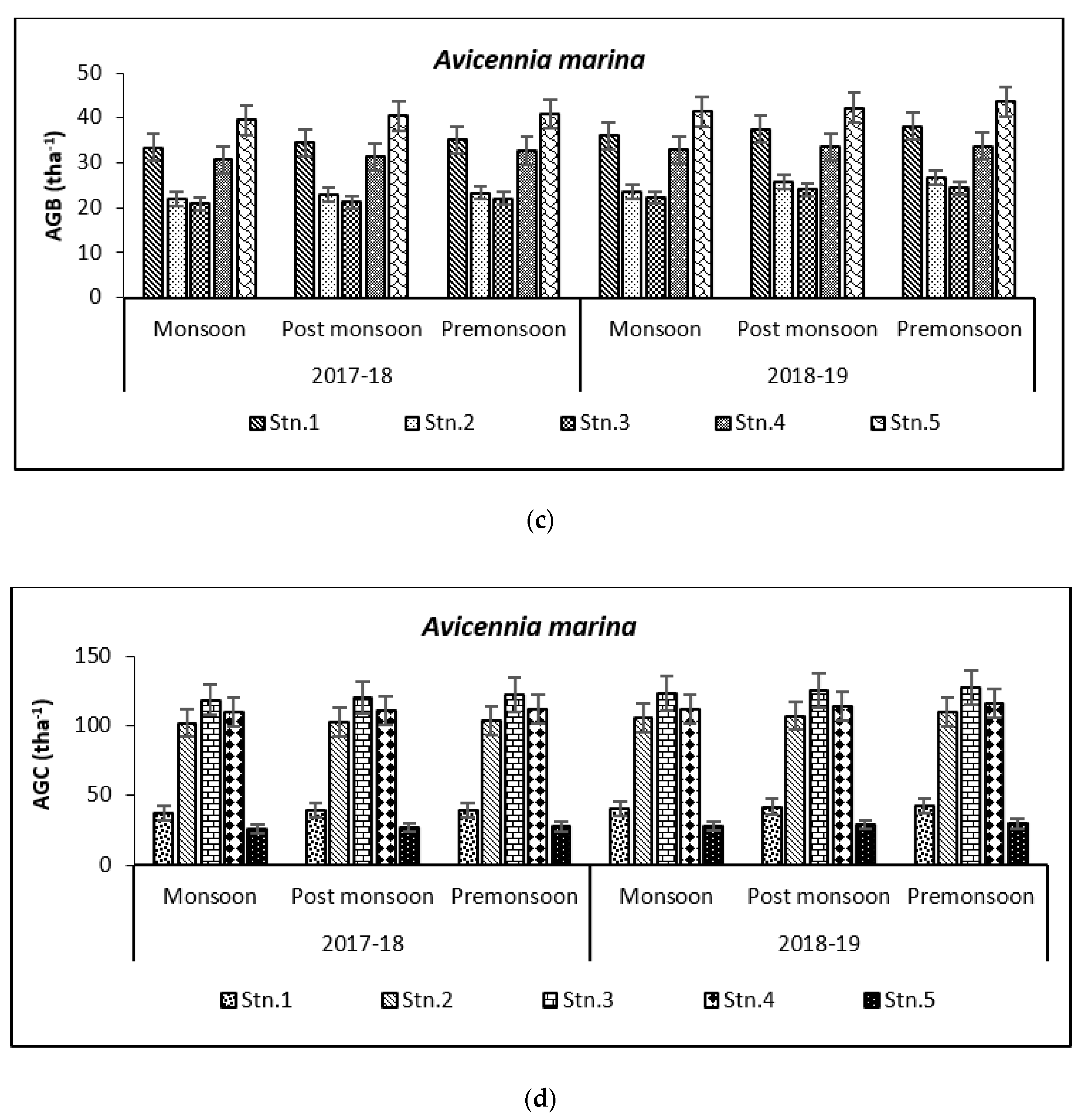
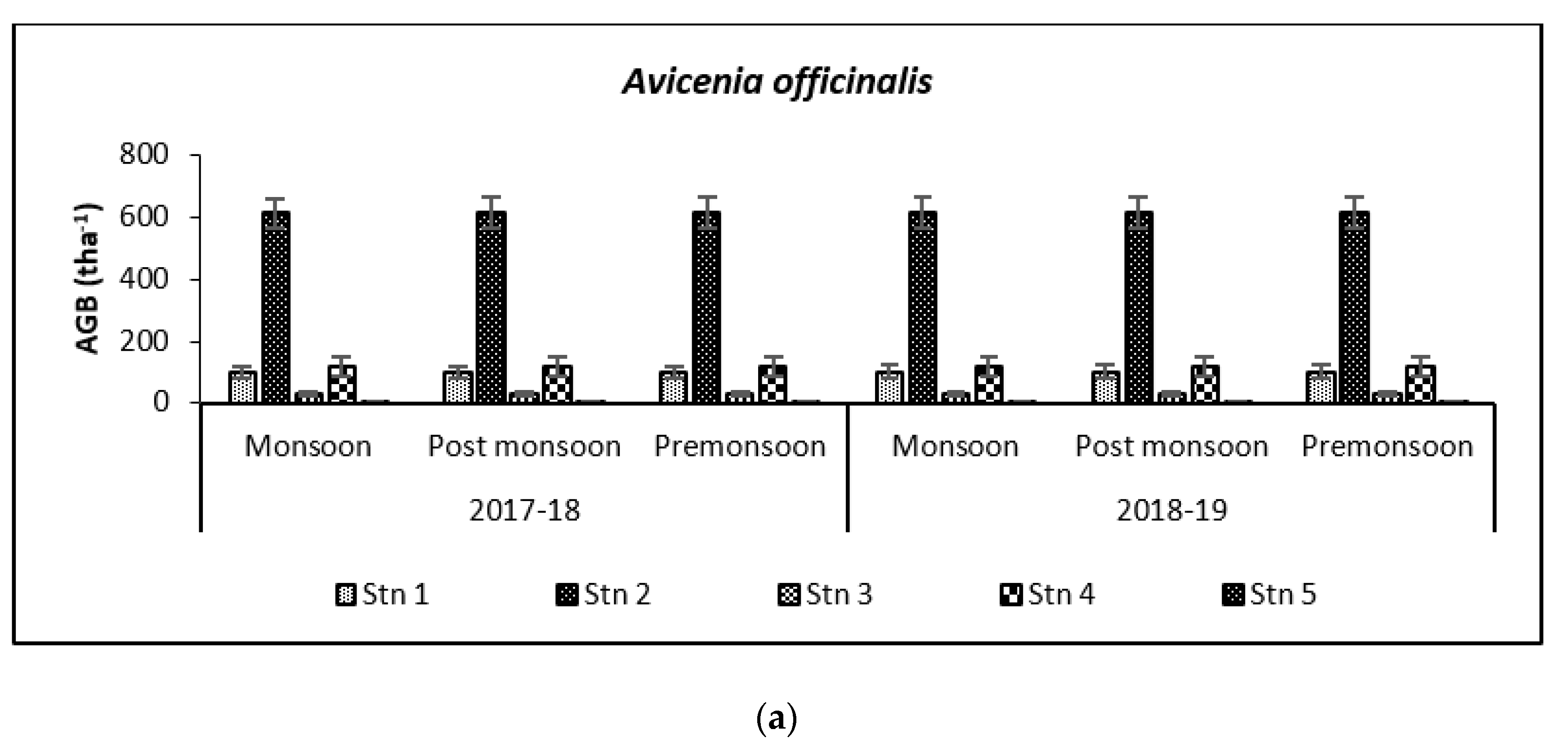
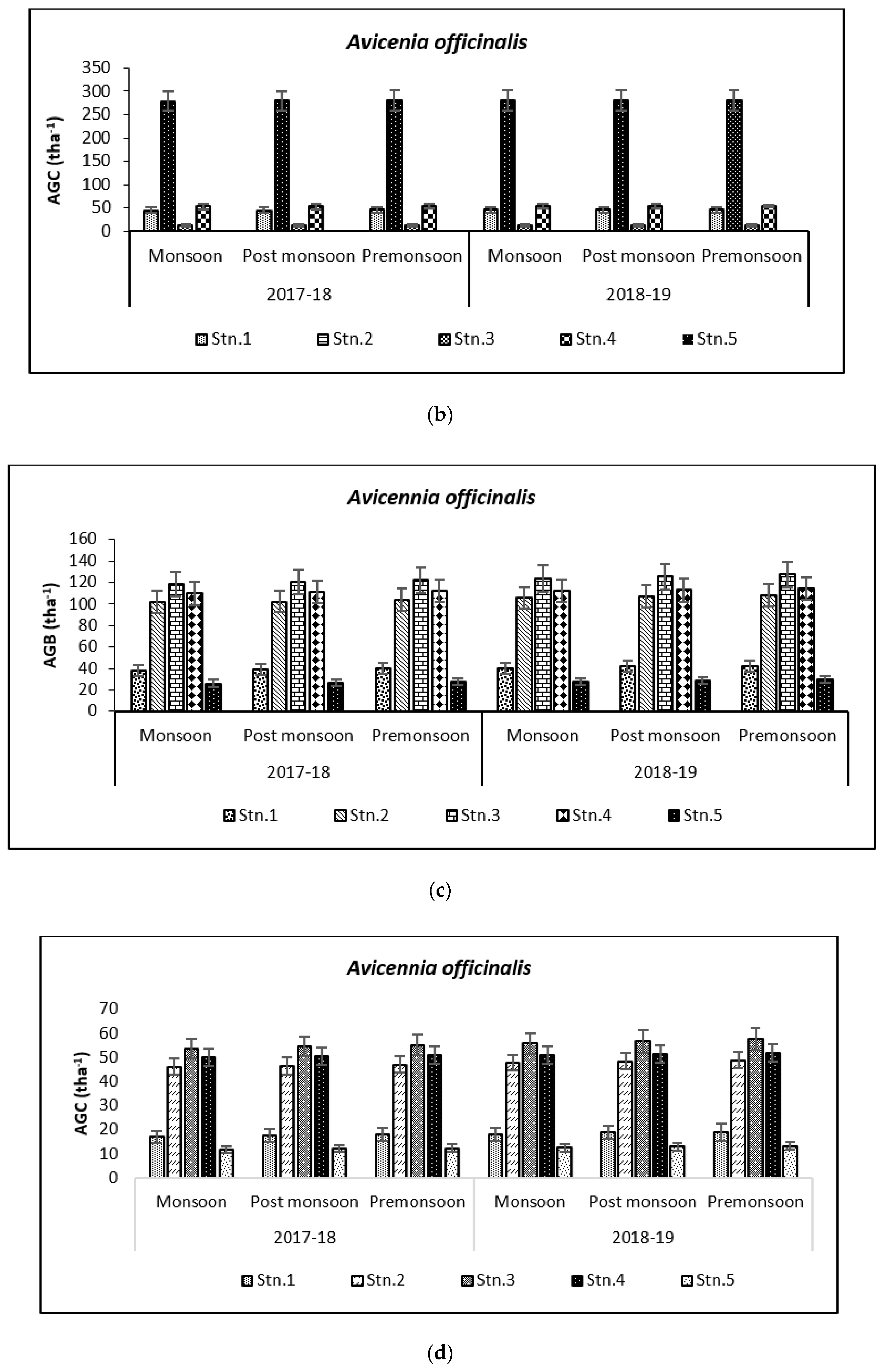
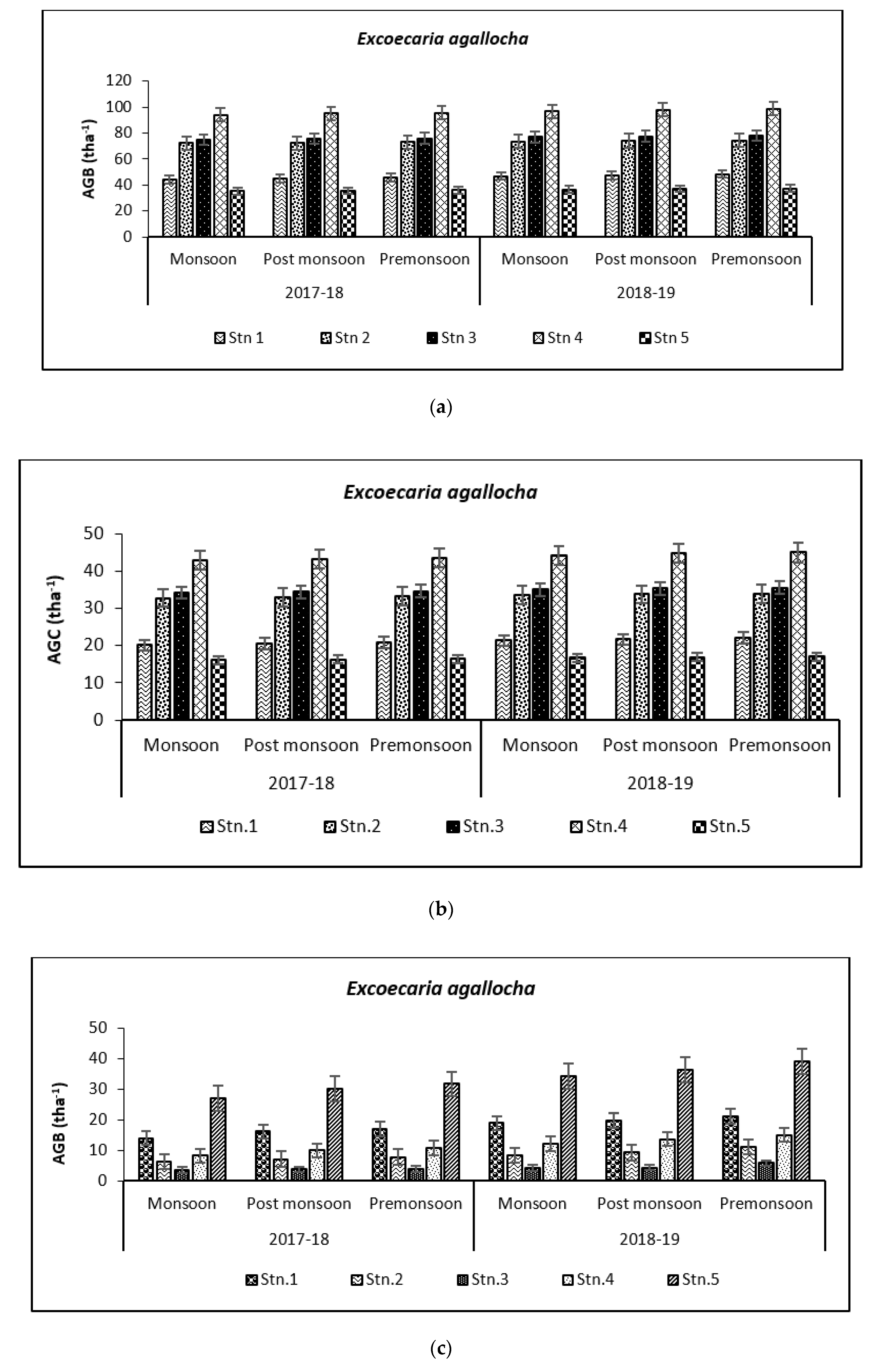
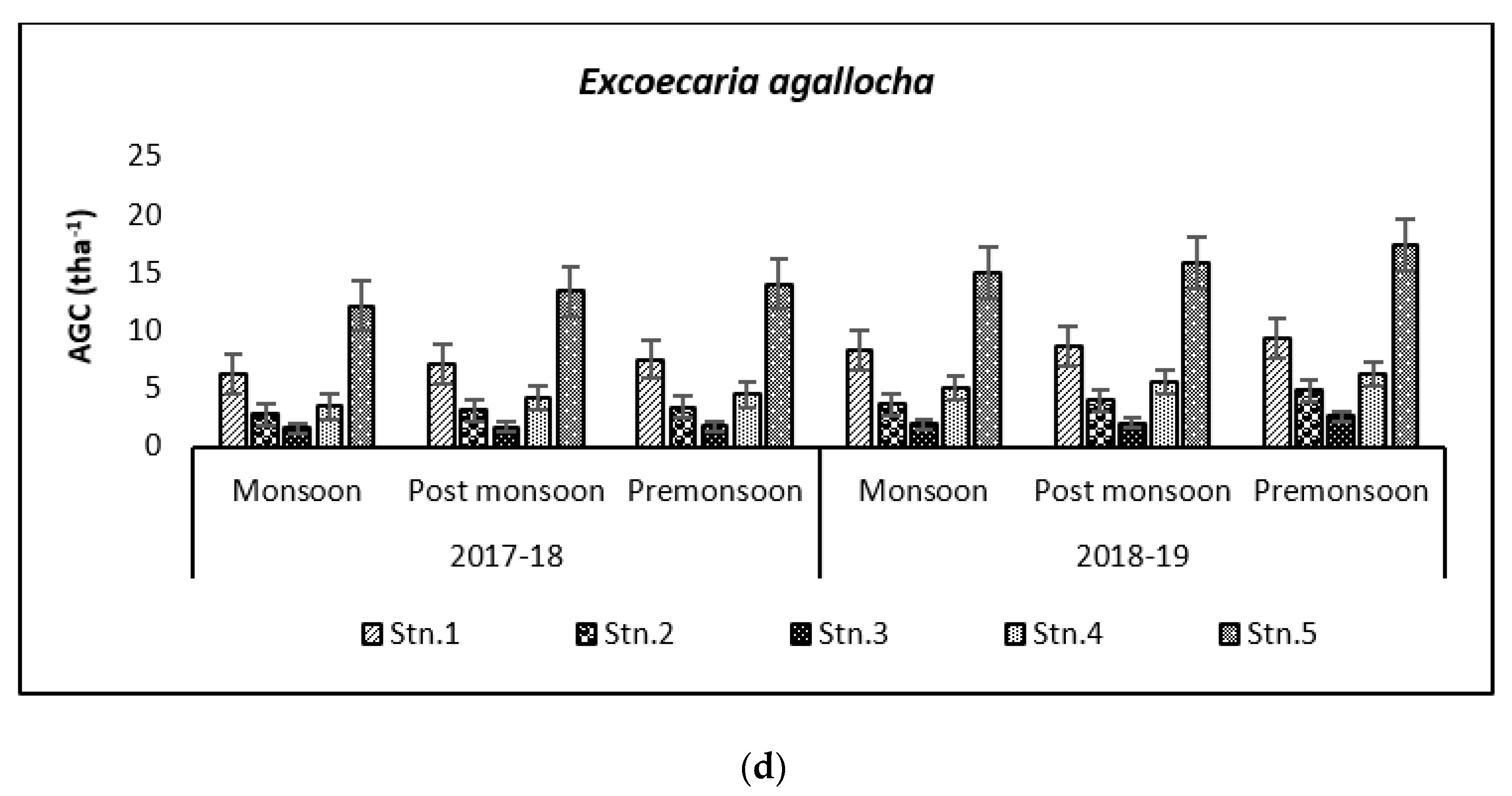
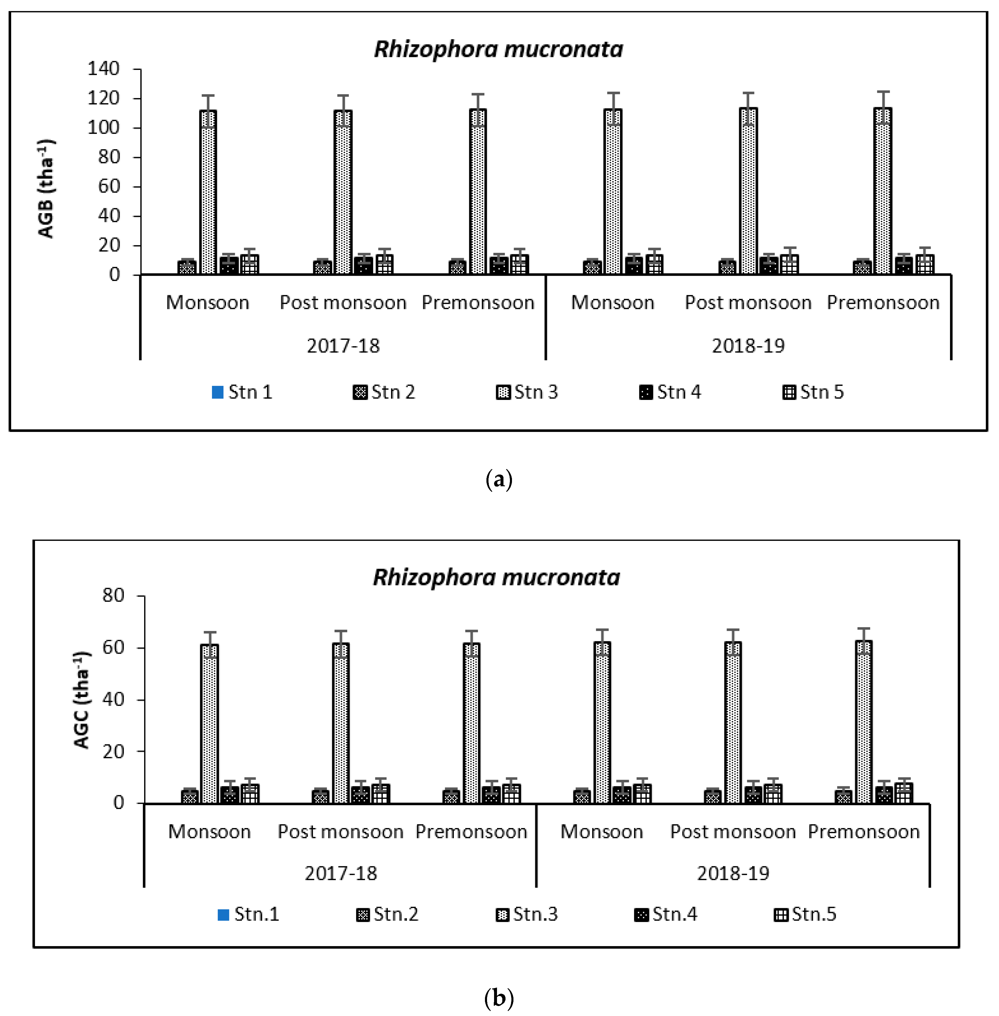
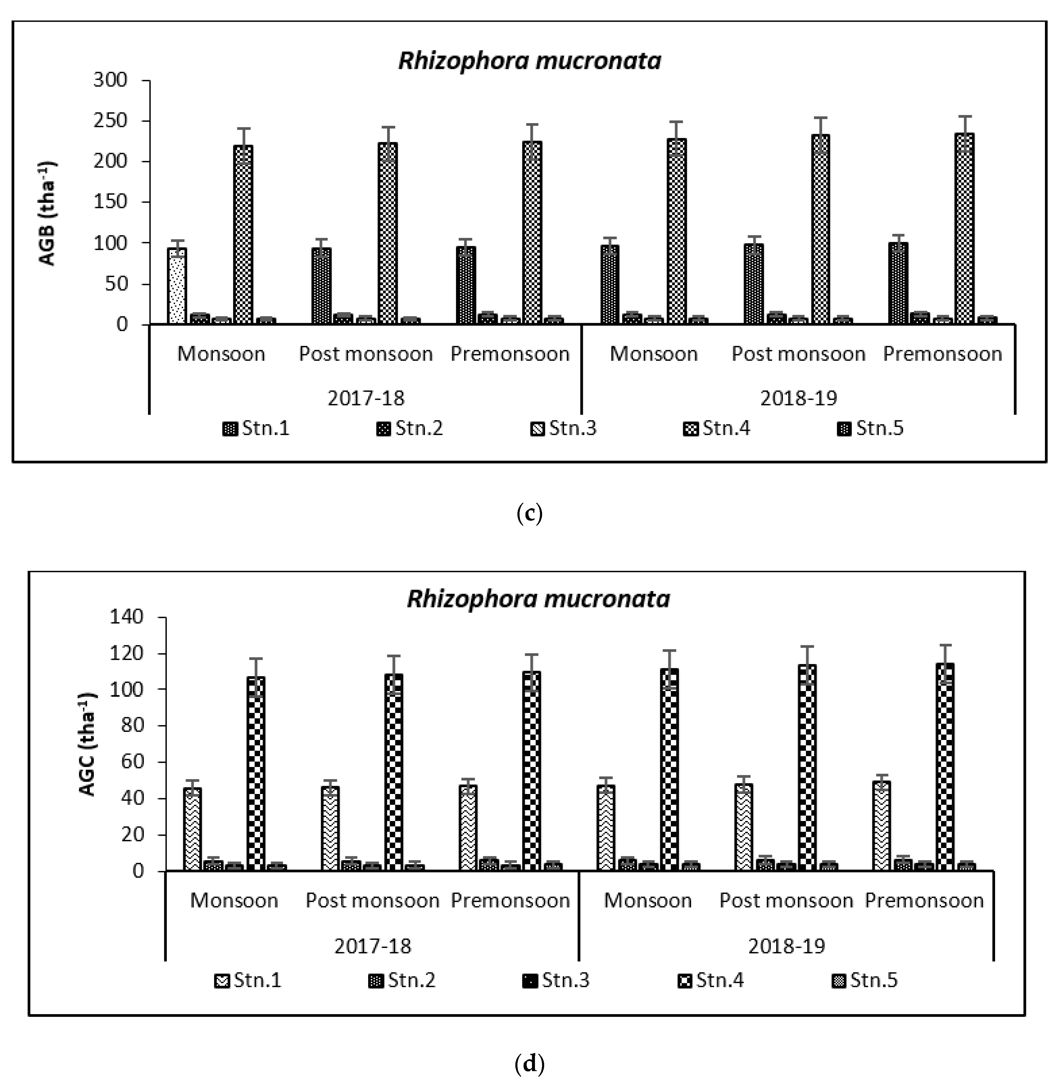
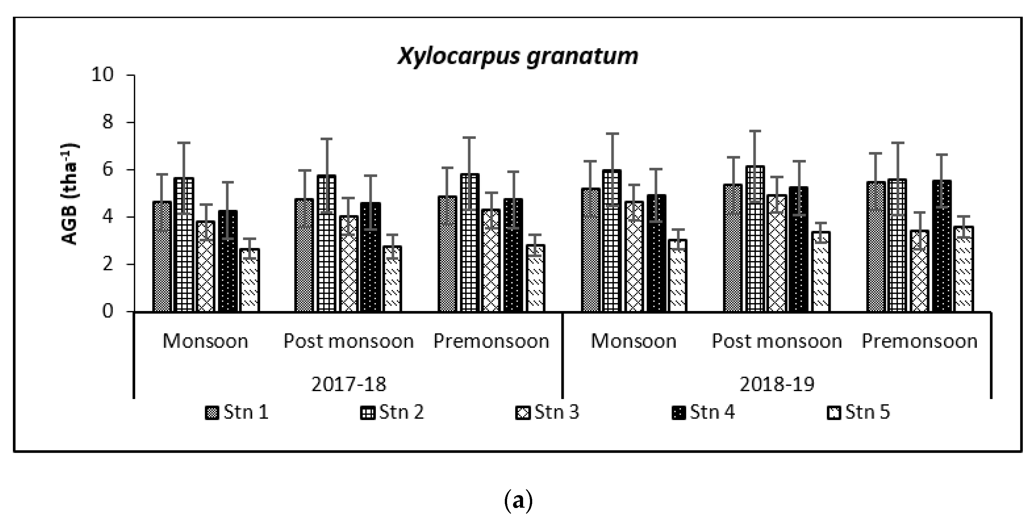
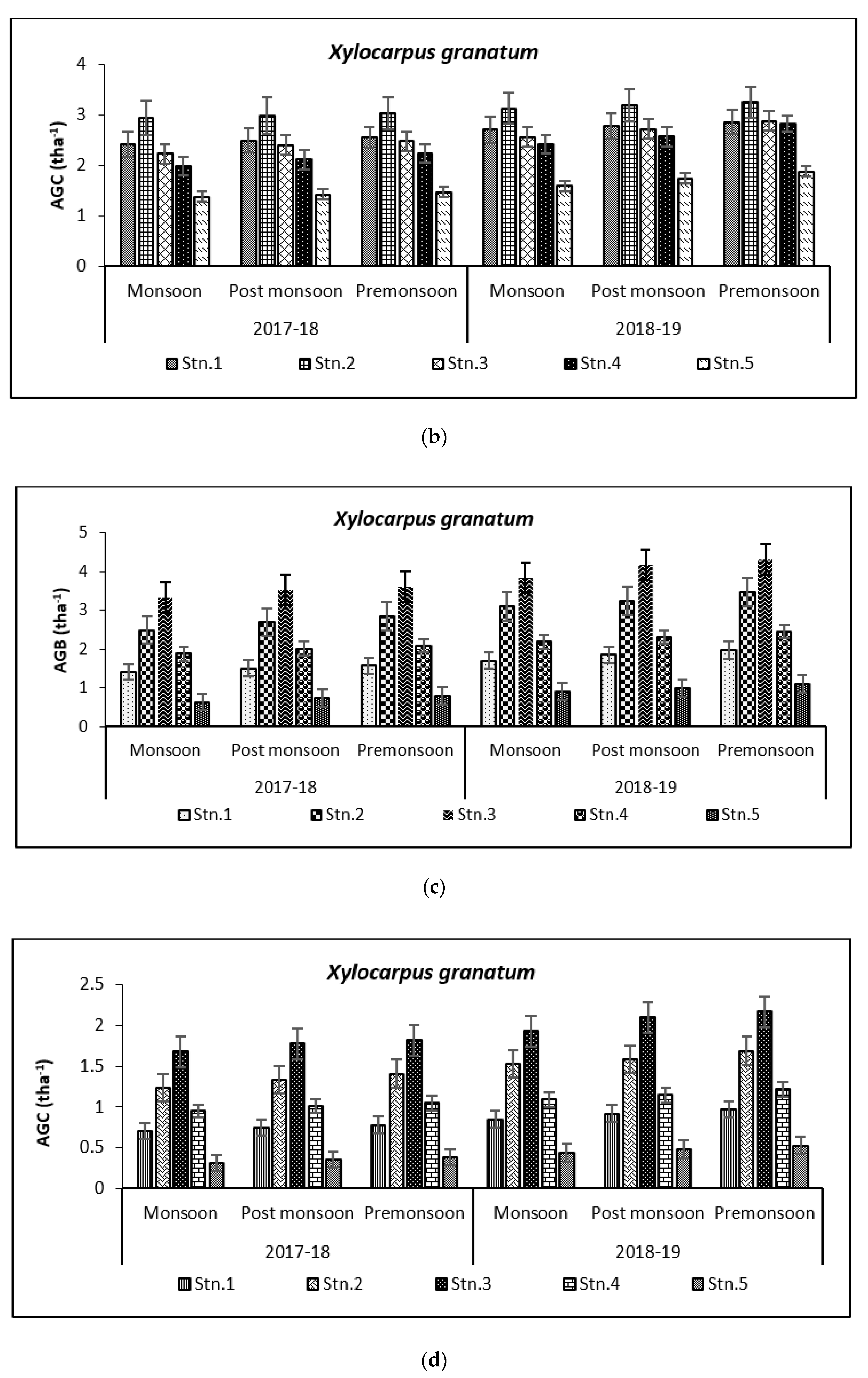
3.2. Carbon Storage in Mangroves (Species Wise)

Above Ground Biomass values ranged from 0.64 ± 0.21 tha−1 for X. granatum to 616.94 ± 50.15 tha−1 for A. officinalis in the study area. Similarly, the Above Ground Carbon values also varied from 0.31 ± 0.10 tha−1 for X. granatum to 280.83 ± 21.29 tha−1 for A. offficinalis (Figure 4, Figure 5, Figure 6, Figure 7 and Figure 8). Spatial variation between the five species that were selected showed the highest value of AGB for A. officinalis at Bhitarkanika and R. mucronata at Mahanadi, while E. agallocha showed almost a uniform growth pattern. Comparing all the species and all the stations, the biomass per hectare of E. agallocha was the highest owing to its high adaptability. This has been proved by significant MANOVA values between stations (p < 0.05) although the variation was insignificant between seasons. Biomass contribution by stem varied from 42.51 ± 21.22% to 89.53 ± 4.30% branch from 9.91 ± 3.67% to 39.97 ± 20.69% and leaf contribution to 0.90 ± 0.47% to 7.65 ± 3.76% and stilt root contributed 29.52 ± 1.11% to 34.14 ± 16.10% (Table 2 and Table 3), respectively.
Species-wise, the average carbon storage over two years (2017–2018 and 2018–2019) were of the order E. agallocha > R. mucronata > A. marina > A. officinalis > X. granatum respectively (Figure 4, Figure 5, Figure 6, Figure 7 and Figure 8). MANOVA results showed significant variation of AGC in context to stations for all species in the selected study area which is at par with the AGB values (Table 4). The percentage of carbon in the floral components in the Bhitarkanika mangrove ecosystem for the different species is given in Table 1, where stem carbon varied from 23.81 ± 11.88% to 41.12 ± 6.57%, branch carbon varies from 9.78 ± 5.40% to 17.99 ± 9.31% and leaf carbon varied from 0.80 ± 0.45% to 3.39 ± 1.67% and stilt root comprised of 18.78 ± 8.85% carbon, respectively. In the case of Mahanadi, the percentage of carbon in floral components is given in Table 3, where stem carbon varied from 23.35 ± 10.28% to 40.92 ± 5.17%, branch carbon varied from 3.89 ± 2.49% to 12.33 ± 5.31%, and leaf carbon varied from 0.37 ± 0.18% to 3.37 ± 1.32% and stilt root comprised of 14.02 ± 5.84% carbon, respectively.
It has been reported that biomass values can be even more than 250 tha−1 [23] in forests with no anthropogenic interferences. Our results are comparable with that in the Sundarbans [24,25], Japan [26], Australia [27], Senegal [28], Guade–loupe [29], Puerto Rico [30], Thailand [31], Florida [32], the Indian Bay of Bengal [33], Indonesia [34], Malaysia [35], Sri Lanka [36], Andaman Islands [37], and Philippines [38]. In the present study, the diurnal inundation of tides was dominated by A. marina, R. mucronata, and E. agallocha because all the three species dominated in high saline areas of the selected stations.
Spatial dependence of AGB with SOC in this western Bay of Bengal mangrove ecosystem is displayed by significant negative relationship (p < 0.01) of AGB with SOC in case of A. marina and positive relationship in context to AGB with SOC at 1% level of significance for A. officinalis and X. granatum respectively. R. mucronata being a more adaptive species with respect to acidity or alkalinity of the soil, showed no relationship for AGB with SOC, with the exception of E. agallocha at a mangrove patch near Mahanadi, which showed a significant negative relationship like A. marina at 5% level of significance. Ren et al. [39] also supported this view for the widespread distribution of the species to changes in SOC composition.
Biomass and carbon in mangroves are a directly proportional relationship, although the percentage of carbon in biomass differs (23.35% to 41.12%) with the age and growth type of the species. More salinity leads to less carbon due to less biomass. The global carbon cycle is very much dependent on this blue carbon, out of which mangroves contribute only a mere 0.7% of tropical forests of the world. These forests have the potential to store up to 20 billion tons of carbon, which is much higher than the carbon stock in tropical upland, temperate, and boreal forests [33]. Mangrove forests contribute a significant proportion to the global carbon cycle as they play a major role in reducing greenhouse gases (viz. CO2) through the process of photosynthesis.

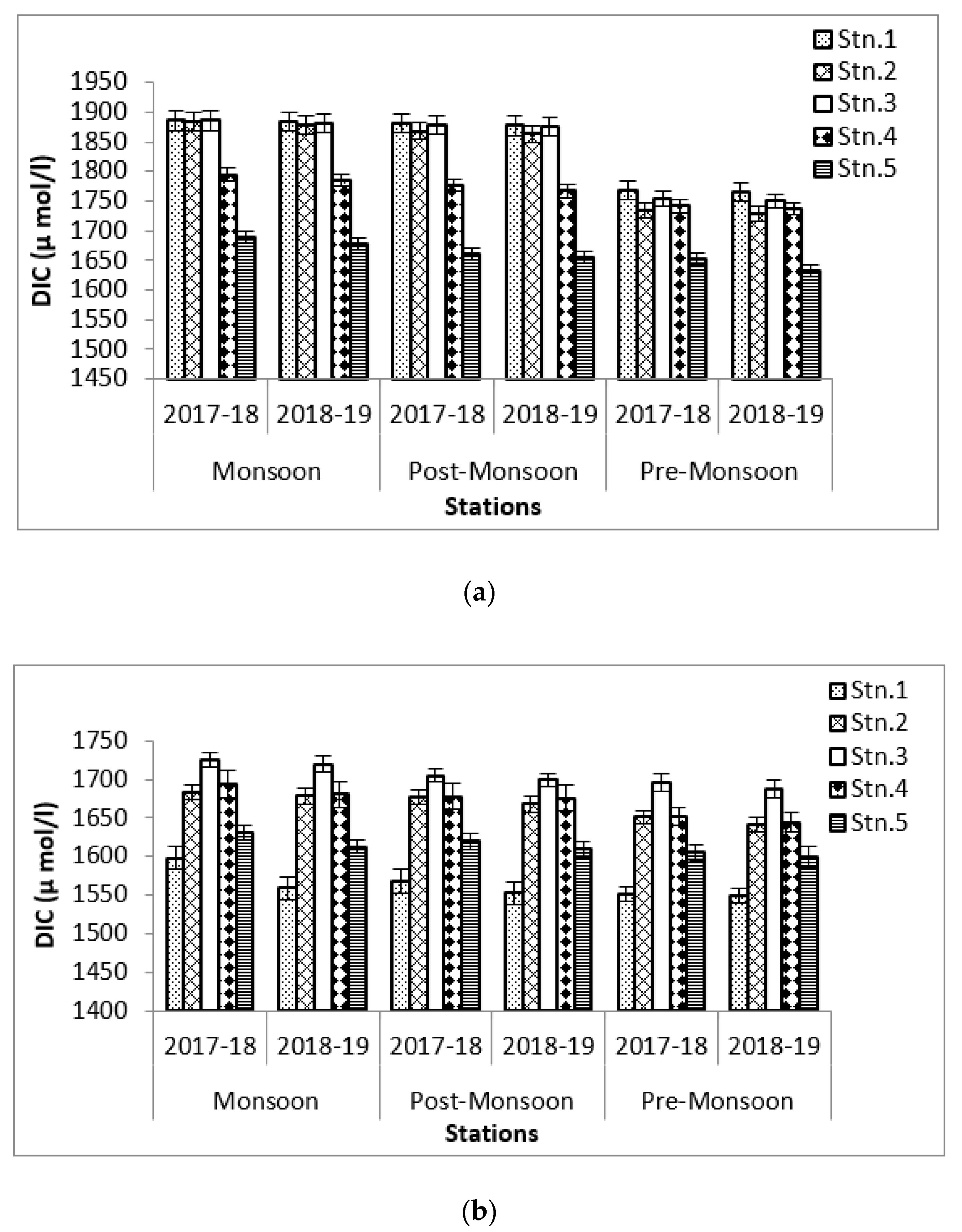
3.3. Carbon Storage in Aquatic Medium

Dissolved Inorganic Carbon (DIC) was monitored in the adjacent waters which are also the sink of carbon dioxide. The amount of carbon in the inorganic state in ambient media is also the contribution of the physico-chemical and microbial interactions (mineral complex) that occur in mangrove sediment [40,41]. The microbial biomass utilizes this newly added carbon in water leading to various metabolic byproducts [42]. These processes help in stabilizing soil organic carbon fraction and nutrient acquisition [43]. Several previous studies have also shown that there is a loss of organic carbon to adjacent saline water [44].
The present study shows that DIC values vary from 1632 ± 9.37 during premonsoon 2018–2019 at Stn.5 to 1887 ± 16.82 µmol/Lduring monsoon 2017–2018 at Stn.1 at Bhitarkanika and from 1549 ± 8.88 during premonsoon 2018–2019 at Stn.1 to 1632 ± 9.56 µmol/L during 2017–2018 at Stn.5 at Mahanadi (Figure 9). The data shows that increase in DIC is inversely proportional to the pH of seawater and positively proportional to SOC because of its dependency on seawater buffer capacity (Figure 10). The other facts on the change are due to the mixing and air-sea interaction through diffusion [45].

3.4. Prospects in Carbon Storage (Whole Ecosystem)

The ability of carbon storage in the mangrove patches in the western Bay of Bengal accounts for the highest (314.76 ± 110.34 tha−1) at Bhitarkanika WLS and lowest (45.96 ± 6.52 tha−1) at Mahanadi estuarine complex, with mean SOC (in tha−1) of 5.69 ± 1.61.
Total carbon (TC) amounts 51.35 ± 6.77 tha1 to 322.47 ± 110.79 tha1 with an average quantity of 141.56 ± 37.01 tha1 at Bhitarkanika and 94.21 ± 20.78 tha1 for Mahanadi mangrove ecosystem, respectively. Spatial CO2e varied from 225.08 ± 45.43 tons to 1183.46 ± 406.60 tons with a mean CO2e of 519.53 ± 135.83 tons for Bhitarkanika and from 188.45 ± 24.85 tons to 666.29 ± 155.68 tons with mean CO2e of 345.75 ± 76.26 tons at Mahanadi respectively (Table 3). Species-wise CSR (carbon sequestration rate) calculated in the study area were A. officinalis (197.26 tha1year1), R. mucronata (85.43 tha1year1), E. agallocha (74.89 tha1year1), A. marina (37.53 tha1year1), and X. granatum (6.10 tha1year1) respectively. Considering the fact that the amount of carbon in the atmosphere is 750 GT and the total flux out (105 Gt to ocean + 110 Gt to life on land) (http://newmaeweb.ucsd.edu accessed on 4 June 2021), the residence time of carbon is 6.81 years on land and 7.14 years on the ocean. Similarly, in the present study, in the Bhitarkanika and Mahanadi mangrove ecosystems separately, the residence time for carbon on land is 3.67 and 3.48 years respectively, whereas it is 45.09 × 10⁵ and 32.64 × 10⁵ years in the ocean, respectively. This proves that the mangrove wetlands play a significant role in governing the carbon cycle.

4. Conclusions

A large proportion of mangrove carbon is unaccounted for in global budgets in climate regulation projects. This present paper has accounted for the amount of carbon that is cycled in mangroves, their adjacent waters, and sediment. The challenge in blue carbon initiatives is to reconcile realistic time frames for its development. The amount of carbon storage in this mangrove ecosystem has been calculated to be 17,655,301.41 ha−1, which will amount to $192.442, considering the carbon price to be $10.90 per ton. The study has tried to highlight the potentiality of the carbon market and the benefits which can be shared among the beneficiaries during plantation projects. The entire study will definitely see the light of implementation if it can be linked with the Clean Development Mechanism (CDM) through the conveyor belt of policy. To achieve the goal of the Paris Climate Agreement through massive plantation, efforts will be required to make a major shift in global priority on the plantation of species with high carbon-storing potential.

Author Contributions

The work has been conceptualized by K.B. and A.M.; methodology, K.B.; software, K.B.; validation, K.B., A.M. and S.V.; formal analysis, K.B.; investigation, K.B.; resources, K.B.; data curation, K.B.; writing—original draft preparation, K.B.; writing—review and editing, A.M. and S.V.; visualization, K.B.; supervision, A.M.; project administration, K.B.; funding acquisition, K.B. All authors have read and agreed to the published version of the manuscript.

Funding

This research was funded by the MINISTRY OF EARTH SCIENCES, GOVT. OF INDIA, grant number MoES/36/OOIS/Extra/44/2015 dated 29 November 2016 nd The APC was funded by S.V.

Institutional Review Board Statement

Not applicable.

Informed Consent Statement

Not applicable.

Data Availability Statement

Not applicable.

Acknowledgments

The authors duly acknowledge Ministry of Earth Sciences, Govt. of India project (Sanction No. MoES/36/OOIS/Extra/44/2015 dated 29 November 2016) for providing financial support. We would like to thank the Institute of Forest Biodiversity, Hyderabad for helping us in analysing the samples. We also thank the Forest Department, Govt. of Odisha for providing necessary permissions to carry on this work. The funding entity for this paper is Xunta de Galicia (Spain).

Conflicts of Interest

The authors declare that there is no conflict of interest.

References

  1. The IUCN Red List of Threatened Species. Available online: http://www.iucnredlist.org. (accessed on 4 January 2019).
  2. Duke, N.C. Mangrove floristics and biogeography. In Tropical Mangrove Ecosystems; Coastal and Marine Estuarine Series 41; Robertson, A.I., Alonghi, D.M., Eds.; American Geophysical Union: Washington, DC, USA, 1992; pp. 63–100. [Google Scholar]
  3. Donato, C.D.; Kauffman, J.B.; Murdiarso, D.; Kurni-Anto, S.; Stidham, M.; Kanninen, M. Mangroves among the most carbon-rich forests in the tropics. Nat. Geosci. 2011, 4, 293–297. [Google Scholar] [CrossRef]
  4. Mathew, G.; Jeyabaskaran, R.; Prema, D. Mangrove ecosystems in India and their conservation. In Coastal Fishery Resources of India-Conservation and Sustainable Utilization; Society of Fisheries Technologists: Kerala, India, 2010; pp. 186–196. [Google Scholar]
  5. Basha, S.K.M.; Indira Priyadarsini, A.; John Paul, M. Mangrove diversity of south east coast of Andhra Pradesh, India. Int. J. Eng. Res. Technol. 2018, 7, 333–337. [Google Scholar]
  6. Naskar, K.; Mandal, R. Ecology and Biodiversity of Indian Mangrove (Part-1: Global Status); Daya Publishing House: Delhi, India, 1999; pp. 1–356. [Google Scholar]
  7. Forest Survey of India (Ministry of Environment and Forests) Dehradun. State Forest Report; Forest Survey of India: Uttarakhand, India, 2017. [Google Scholar]
  8. Sahu, S.C.; Suresh, H.S.; Murthy, I.K.; Ravindranath, N.H. Mangrove area assessment in India: Implications of loss of mangroves. J. Earth Sci. Clim. Chang. 2016, 6, 1–7. [Google Scholar]
  9. Banerjee, K.; Chowdhury, M.R.; Sengupta, K.; Sett, S.; Mitra, A. Influence of anthropogenic and natural factors on the mangrove soil of Indian Sundarbans wetland. Arch. Environ. Sci. 2012, 6, 80–91. [Google Scholar]
  10. Sahoo, K.; Dhal, N.K. Potential microbial diversity in mangrove ecosystems: A review. Indian J. Mar. Sci. 2003, 38, 249–256. [Google Scholar]
  11. Abu Hena, M.K.; Ashrafu, M.A.K. Coastal and estuarine resources of Bangladesh: Management and conservation issues. Maejo Intern J. Sci. Technol. 2009, 3, 313–342. [Google Scholar]
  12. Duarte, C.M.; Losada, I.J.; Hendriks, I.E.; Mazarrasa, I.; Marba, N. The role of coastal plant communities for climate change mitigation and adaptation. Nat. Clim. Chang. 2013, 3, 961–968. [Google Scholar] [CrossRef] [Green Version]
  13. Mitra, A.; Sundaresan, J. How to Study Stored Carbon in Mangroves; CSIR-National Institute of Science Communication: New Delhi, India; Information Resources (NISCAIR): New Delhi, India, 2016; ISBN 978-81-7236-349-9. [Google Scholar]
  14. Walkley, A.; Black, I.A. An examination of the Degtjareff method for determining soil organic matter, and proposed modification of the chromic acid tritation method. Soil Sci. 1934, 37, 29–38. [Google Scholar] [CrossRef]
  15. Edmond, J.M. High precision determination of titration alkalinity and total carbon dioxide content of seawater by potentiometric titration. Deep-Sea Res. 1970, 17, 737–750. [Google Scholar]
  16. Goyet, C.; Beauverger, C.; Brunet, C.; Poisson, A. Distribution of carbon dioxide partial pressure in surface waters of the southwest Indian Ocean. Tellus 1991, 43B, 1–11. [Google Scholar]
  17. D.O.E. Handbook of Methods for Analysis of the Various Parameters of the Carbon Dioxide System in Sea Water, 2nd ed.; Dickson, A.G., Goyet, C., Eds.; ORNL/CDIAC/USDOE: Washington, DC, United States, 1994; p. 74. [Google Scholar]
  18. Das, S.; Ganguly, D.; Maiti, T.K.; Mukherjee, A.; Jana, T.K.; De, T.K. A Depth-wise diversity of free living N2 fixing and Nitrifying Bacteria and its seasonal variation with nitrogen containing nutrients in the mangrove sediments of Sundarbans, WB, India. Open J. Mar. Sci. 2013, 3, 112–119. [Google Scholar] [CrossRef] [Green Version]
  19. Reddy, H.R.V.; Hariharan, V. Distribution of nutrients in the sediments of the Netravathi Gurupur estuary, Mangalore. Indian J. Fish. 1986, 33, 123–126. [Google Scholar]
  20. Sverdrup, H.U.; Johnson, M.W.; Fleming, R.H. The Oceans, Their Physics, Chemistry, and General Biology; Printice Hall, Inc.: Hoboken, NJ, USA, 1942; p. 1087. [Google Scholar]
  21. Mitra, A.; Sengupta, K.; Banerjee, K. Standing biomass and carbon storage of above-ground structures in dominant mangrove trees in the Sundarbans. For. Ecol. Manag. 2011, 261, 1325–1335. [Google Scholar] [CrossRef]
  22. Canadell, J.G.; Pitelka, L.F.; Ingram, J.S.I. The effects of elevated [CO2] on plant-soil carbon below-ground: A summary and synthesis. Plant Soil 1995, 187, 391–400. [Google Scholar] [CrossRef]
  23. Hall, G.M.J.; Wiser, S.K.; Allen, R.B.; Beets, P.N.; Goulding, C.J. Strategies to estimate national forest carbon stocks from inventory data: The 1990 New Zealand baseline. Glob. Chang. Biol. 2001, 7, 389–403. [Google Scholar] [CrossRef]
  24. Joshi, H.G.; Ghose, M. Community structure, species diversity, and aboveground biomass of the Sundarbans mangrove swamps. Trop. Ecol. 2014, 55, 283–303. [Google Scholar]
  25. Banerjee, K. Decadal change in the surface water salinity profile of Indian Sundarbans: A Potential Indicator of Climate Change. J. Mar. Sci. Res. Dev. 2013, 2, 3. [Google Scholar] [CrossRef]
  26. Suzuki, E.; Tagawa, H. Biomass of a mangrove forest and a sedge marsh on Shigaki Island, South Japan. Jpn. J. Ecol. 1983, 33, 231–234. [Google Scholar]
  27. Woodroffe, C.D. Studies of a mangrove basin, Tuff Crater, New Zealand. I: Mangrove biomass and production of detritus, Estuarine. Coast. Shelf Sci. 1985, 20, 265–280. [Google Scholar] [CrossRef]
  28. Doyen, A. La mangrove a usage multiple de I’estuarine Saloum (Senegal). In Selected Papers of the Dakar Symposium on Acid Sulphate Soils; Publication no. 44; Dost, H., Ed.; International Institute for Land Reclamation and Improvement: Wageningen, The Netherlands, 1986; pp. 176–201. [Google Scholar]
  29. Imbert, D.; Rollet, B. Phytomass eaerienneet production primairedans la mangrove du Grand Cul-de-Sac Maria (Guadeloupe, Antilles francaises). Bull. D’écol. 1989, 20, 27–39. [Google Scholar]
  30. Golley, F.; Odum, H.T.; Wilson, R. The structure and metabolism of a Puerto Rican red mangrove forest in May. Ecology 1962, 43, 9–19. [Google Scholar] [CrossRef] [Green Version]
  31. Christensen, B. Biomass and productivity of Rhizophora apiculata B1 in a mangrove in southern Thailand. Aquat. Bot. 1978, 4, 43–52. [Google Scholar] [CrossRef]
  32. Lugo, A.E.; Snedaker, S.C. The ecology of mangroves. Annu. Rev. Ecol. Evol. Syst. 1974, 5, 39–64. [Google Scholar] [CrossRef]
  33. Kathiresan, K.; Gomathi, V.; Anburaj, R.; Saravanakumar, K.; Asmathunisha, N.; Sahu, S.K.; Shanmugaarasu, V.; Anandhan, S. Carbon sequestration potential of Rhizophora mucronata and A. marina as influenced by age, season, growth and sediment characteristics in southeast coast of India. J. Coast Conserv. 2013, 17, 397. [Google Scholar] [CrossRef]
  34. Komiyama, A.; Moriya, H.; Prawiroatmodjo, S.; Toma, T.; Ogino, K. Forest primary productivity. In Biological System of Mangrove; Ogino, K., Chihara, M., Eds.; Ehime University: Matsuyama, Japan, 1988; pp. 97–117. [Google Scholar]
  35. Putz, F.; Chan, H.T. Tree growth, dynamics, and productivity in a mature mangrove forest in Malaysia. For. Ecol. Manag. 1986, 17, 211–230. [Google Scholar] [CrossRef]
  36. Amarasinghe, M.D.; Balasubramaniam, S. Net primary productivity of two mangrove forests stands on the northwest coast of Sri Lanka. Hydrobiologia 1992, 247, 37–47. [Google Scholar] [CrossRef]
  37. Mall, L.P.; Singh, V.P.; Garge, A. Study of biomass, litter fall, litter decomposition and soil respiration in monogenetic mangrove and mixed mangrove forests of Andaman Islands. Trop. Ecol. 1991, 32, 144–152. [Google Scholar]
  38. Camacho, L.D.; Gevana, D.T.; Carandang, A.P.; Camacho, S.C.; Combalicer, E.A.; Rebugio, L.L.; Youn, Y.C. Tree biomass and carbon stock of a community managed mangrove forest in Bohol, Philippines. For. Sci. Technol. 2011, 7, 161–167. [Google Scholar] [CrossRef]
  39. Ren, H.; Chen, H.; Li, Z.A.; Han, W. Biomass accumulation and carbon storage of four different aged Sonneratia apetala plantations in Southern China. Plant Soil 2010, 327, 279–291. [Google Scholar] [CrossRef]
  40. Plaza, C.; Courtier-Murias, D.; Fernandez, J.M.; Polo, A.; Simpson, A.J. Physical, chemical and biochemical mechanisms of soil organic matter stabilization under conservation tillage systems: A central role for microbes and microbial by-products in C sequestration. Soil. Biol. Biochem. 2013, 57, 124–134. [Google Scholar] [CrossRef] [Green Version]
  41. Justrow, J.; Miller, R. Soil Processes and the Carbon Cycle; Rattan Lal, J.M.K., Ronald, F.F., Bobby, S., Eds.; CRC Press: Boca Raton, FL, USA, 1997; pp. 207–223. [Google Scholar]
  42. Cotrufo, M.F.; Soong, J.L.; Horton, A.J.; Campbell, E.E.; Haddix, M.L.; Wall, D.H.; Parton, W.J. Formation of soil organic matter via biochemical and physical pathways of litter mass loss. Nat. Geosci. 2015, 8, 776–779. [Google Scholar]
  43. Kuzyakov, Y.; Friedel, J.K.; Stahr, K. Review of mechanisms and quantification of priming effects. Soil Biol. Biochem. 2000, 32, 1485–1498. [Google Scholar] [CrossRef]
  44. Conde, E.; Cardenas, M.; Ponce-Mendoza, A.; Luna-Guido, M.L.; Cruz-Mondragón, C.; Dendooven, L. The impacts of inorganic nitrogen application on mineralization of 14C labelled maize and glucose, and on priming effect in saline alkaline soil. Soil Biol. Biochem. 2005, 37, 681–691. [Google Scholar] [CrossRef]
  45. Olafsson, J.; Olafsdittir, S.R.; Benoit-Cattin, A.; Takahashi, T. The Irminger sea and the Iceland sea time series measurements of sea water carbon and nutrient chemistry 1983–2008. Earth Syst. Sci. Data 2010, 2, 99–104. [Google Scholar] [CrossRef] [Green Version]
Figure 1. Schematic representation of carbon cycling in the western Bay of Bengal.
Sustainability 13 06740 g001
Figure 2. Western Bay of Bengal map showing Bhitarkanika WLS and Mahanadi estuarine complex.
Sustainability 13 06740 g002
Figure 3. Graph showing variation in soil OC (%) in (a) Bhitarkanika and (b) Mahanadi estuarine complex.
Sustainability 13 06740 g003aSustainability 13 06740 g003b
Figure 4. Graph showing biomass (tha−1) (a) and carbon (tha−1) (b) in Bhitarkanika WLS. Graph showing biomass (tha−1) (c) and carbon (tha−1) (d) in Mahanadi estuarine complex.
Sustainability 13 06740 g004aSustainability 13 06740 g004b
Figure 5. Graph showing biomass (tha−1) (a) and carbon (tha−1) (b) in Bhitarkanika WLS. Graph showing biomass (tha−1) (c) and carbon (tha−1) (d) in Mahanadi estuarine complex.
Sustainability 13 06740 g005aSustainability 13 06740 g005b
Figure 6. Graph showing biomass (tha−1) (a) and carbon (tha−1) (b) in Bhitarkanika WLS. Graph showing biomass (tha−1) (c) and carbon (tha−1) (d) in Mahanadi estuarine complex.
Sustainability 13 06740 g006aSustainability 13 06740 g006b
Figure 7. Graph showing biomass (tha−1) (a) and carbon (tha−1) (b) in Bhitarkanika WLS. Graph showing biomass (tha−1) (c) and carbon (tha−1) (d) in Mahanadi estuarine complex.
Sustainability 13 06740 g007aSustainability 13 06740 g007b
Figure 8. Graph showing biomass (tha−1) (a) and carbon (tha−1) (b) in Bhitarkanika WLS. Graph showing biomass (tha−1) (c) and carbon (tha−1) (d) in Mahanadi estuarine complex.
Sustainability 13 06740 g008aSustainability 13 06740 g008b
Figure 9. Graph showing DIC values (µmol/L) (a) at Bhitarkanika WLS and (b) at Mahanadi estuarine complex.
Sustainability 13 06740 g009
Figure 10. Relationship of DIC with SOC and water pH at the study site.
Sustainability 13 06740 g010
Table 1. (a) Station description of Bhitarkanika mangrove ecosystem. (b) Station description of Mahanadi mangrove ecosystem.
StationsCoordinatesSite Description
Latitude (N)Longitude (E)
(a)
Stn.120°44′21.37″86°52′00.00″It is a protected mixed natural mangrove forest dominated by H. fomes, E. agallocha, and A. officinalis. The vegetation has a mean stand density of 60 trees per 100 m2, mean DBH is 0.50 m, and mean height of 12 m. The area is a tourist site that receives a freshwater discharge from rivers like Bramhani, Baitarani, and the distributaries of Bhitarkanika river and different creeks, channels, etc. Eighty percent of crocodile nesting occurs here and it has huge reptile diversity like snakes, turtles, monitor lizards, etc. Owing to dense mangrove vegetation, the sediment is often black in color.
Stn.220°42′56.85″86°51′48.40″This site is similar to Dangmal in all conditions (climatic, vegetation, and river-fed) but it is more pristine and undisturbed w.r.t mangrove habitat. This site is famous for crocodile nesting and bird watching sites, Baga–gahana. The biomass of the A. officinalis is very high in comparison to all other study sites. The vegetation has a mean stand density of 80 trees per 100 m2, mean DBH is 0.60 m, and mean height of 12 m. The soil is also very rich in organic matter derived from mangrove litter.
Stn.320°38′38.81″86°52′20.29″This site is an anthropogenically stressed area in comparison to other stations. The area is mostly surrounded by villages and agriculture and aquaculture are the main occupations of the residents. Other activities include ecotourism, transportation, fishing, and household pollution. This is the gateway for BWLS. The distributions of mangrove species are unequal and are found in patches due to cutting and plantation. The dominant species include P. paludosa, E. agallocha and R. mucronata. The vegetation has a mean stand density of 70 trees per 100 m2, mean DBH is 0.40 m, and mean height of 8 m. This site also comes under subtropical and humid climatic zones. The area receives a lot of anthropogenic wastes from adjoining villages, agriculture, and aquaculture discharges.
Stn.420°41′08.12″86°59′16.03″The site is near the sea mouth. One side is open to the Bay of Bengal and the other side is on the bank of river Bausagada. Both the ends of this river are open to the sea, hence it is always tide fed and maintains higher salinity than other study stations. This site also faces anthropogenic pressures like cutting of forest trees, fishing, ecotourism, and other anthropogenic effects. Plastic pollution is very high on this site, mostly on the oceanic coast. The area was dominated by E. agallocha, A. marina, L. racemosa and C. decandra. The vegetation has a mean stand density of 180 trees per 100 m2, mean DBH is 0.30 m, and mean height 6 m. Owing to the position of the station, the station is very dynamic with fresh water on one side and marine water on the other. Organic matter load is comparatively higher.
Stn.520°42′16.91″86°01′56.34″The site is called Ekakula, which means one mouth is open to the rivers Bausagada and Patsala. Both sides are open to the Bay of Bengal, hence it always maintains the highest salinity. The site is dominated by high salt-tolerant species like A. marina, E. agallocha, A. corniculatum, A. rotundifolia, A. alba, R. mucronata, and S. alba. The vegetation has a mean stand density of 120 trees per 100 m2, the mean DBH is 0.15 m, and the average height of the tree is below 7 m but the density of the species is more. The soil is usually loose, sandy in character, but due to the high density of mangroves has rich litterfall.
(b)
Stn.120°25′50.05″86°43′50.21″It is a Proposed Forest (PF) block with an area of 369.75 ha and surrounded by the Gobari river in the south and Chataka in the east, Kandarapatia PRF block in the north, and Gobari river with Jambu village in the west. The waterway plays an important role by inundating the forest block diversity. The dominant species are Avicennia marina Ceriops decandra, Excocecaria agallocha, Acanthus ilicifolius and Avicennia officinalis. Aegiceras corniculatum, Avicennia alba, and Rhizophora mucronata are also found in small numbers. Xylocarpus granatum is rare in this site. Dalbergia spinosa, Sonneratia apetala, Tamarix troupii, Aegialitis rotundifolia and Phoenix paludosa are found in this forest block. One of the non-mangrove species Casuarina species forest patches is also found in this region. The vegetation has a mean stand density of 55 trees per 100 m2, mean DBH is 0.60 m, and mean height 10 m. The forest block is degraded by agricultural runoff, anthropogenic activity, shrimp culture, and grazing.
Stn.220°22′48.89″86°45′09.31″This forest block is the highest area among the selected study sites which comprises about 1394.744 ha. This study site comes under Proposed Reserved Forest (PRF) block. Distributaries of the Gobari river play a crucial role in mangrove growth and regeneration. Kharnasi River separates Kansaridia and Bhitara Kharnasi forest block in the west and one of the creek formations called Kalpana Jore, in the northern part nearer to the Bay of Bengal called as the Chataka and extending to the east. In the southern part, Hetamundia forest and Kajalapatia village are present.
Excoecaria agallocha is the dominant species on this site. Rhizophora mucronata, Ceriops decandra, and Brownlowia tersa are mostly dominant in the area. Xylocarpus granatum, Rhizophora apiculata, Avicennia officinalis, Avicennia marina and Dalbergia spinosa are moderately distributed. Apart from that other species present are Agiceras corniculatum, Acanthus ilicifolius, Sonneratia apetala, Avicennia alba, Kandelia candel, Bruguiera cylindrical and Bruguiera gymnorrhiza. The vegetation has a mean stand density of 50 trees per 100 m2, mean DBH is 0.35 m, and mean height of 7 m. The forest block exhibits rich species diversity but it is in a degraded state due to anthropogenic activity and overexploitation.
Stn.320°22′03.197″86°43′13.18″Kharnasi forest block is classified as Bhitara Kharnasi Reserved Forest (RF-A) and Bahara Kharinasi Reserved Forest (RF-B). Our study site is the Bhitara Kharnasi (RF-A), which has a total area of 577.072 ha. It is surrounded by the distributaries of Kharnasi river and Gobari river which meet the Bay of Bengal. Kharnasi River separates the Bhitara Kharnasi and Bahara Kharnasi in the western part. In the north, the name of the water body is called Chataka which connects with the Bay of Bengal. Kansaridia and Sanatubi forest blocks are present in the east and south respectively. Distributaries play an important role by flushing fresh water inside the region and making it a dense forest.
Excocecaria agallocha is a dominant species in this region followed by Avicennia officinalis, Heritiera fomes, Brownlowia tersa, Ceriops decandra, Rhizophora mucronata, Avicennia marina and Xylocarpus granatum are small in number along with Sonneratia apetala, Avicennia alba, Bruguiera gymnorrhiza and Phoenix paludosa. The vegetation has a mean stand density of 80 trees per 100 m2, mean DBH is 0.45 m, and mean height of 9 m. Anthropogenic activities, shrimp culture, and polluted agricultural flushing by the waterways are the main reasons for the diminishing of mangrove growth.
Stn.420°27′53.61″86°41′15.41″This forest block comes under the Reserve Forest (RF) block with an area of about 137.784 ha. This forest patch is a mixture of natural and plantation forests. The plantation program was done by MSSRF with the help of local villagers and the Forest department of Odisha. The forest block is surrounded by the Gobari river in the south, the Chataka and distributaries of the Jagjore river in the east and north respectively, and Kantilo village with Luna nai which falls in the Gobari river in the western part of the forest block. To get a sufficient tidal inundation, canals have been excavated in the Kantilo forest block.
The dominant species at this site is Rhizophora mucronata. Avicennia marina, Avicennia officinalis, Excocecaria agallocha are also found in numbers. Xylocarpus granatum is rare and Ceriops decandra, Agiceras corniculatum, Acanthus ilicifolius, Sonneratia apetala, Avicennia alba, Kandelia candel, Tamarix troupii, Phoenix paludosa, Bruguiera parviflora and Sonneratia alba are also found in the region. The vegetation has a mean stand density of 150 trees per 100 m2, mean DBH is 0.30 m, and mean height of 8 m.
The main causes of mangrove destruction are anthropogenic activities, agricultural runoff, grazing, shrimp culture and plastics, polythene, etc., inside the forest area.
Stn.520°26′52.77″86°43′32.83″This forest block comes under the Proposed Reserve Forest (PRF), which has represented an area of about 105.668 ha. It is surrounded by Jambu forest block in the south, the Bay of Bengal in the east (Chataka), the Jagajhore river at Jagajhore in the north, and Kandarapatia village with a non-mangrove land patch in the west. The forest block is inundated during high tide which is favorable for the distribution of species composition.
Excoecaria agallocha is dominant in the study area followed by Avicennia marina and Avicennia officinalis along with Ceriops decandra. A very small number of Rhizophora mucronata is found near the saline embankment of the site. Xylocarpus granatum is rare in this region. Other species found are Aegiceras corniculatum, Avicennia alba, Bruguiera cylindrica, Tamarix troupii, Aegialitis rotundifolia, Phoenix paludosa and Pongamia pinnata. The vegetation has a mean stand density of 70 trees per 100 m2, a mean DBH is 0.30 m, and a mean height of 7 m. Runoff from agricultural land, polluted water from shrimp culture, grazing, and anthropogenic activities are the main cause for the destruction of this dense mangrove patch.
Table 2. Percentage sharing of floral components of AGB and AGC at Bhitarkanika WLS.
SpeciesBiomass Contribution by Different Floral Components towards AGB (in %)Carbon Contribution by Different Floral Components towards AGC (in %)
StemBranchLeafStilt RootsStemBranchLeafStilt Roots
A. marina63.01 ± 19.1634.45 ± 17.922.54 ± 1.3828.98 ± 8.8115.16 ± 7.881.07 ± 0.58
(46 ± 0.4) *(44 ± 0.3) *(42 ± 0.4) *
A. officinalis77.58 ± 12.3920.81 ± 11.501.61 ± 0.9041.12 ± 6.579.78 ± 5.400.80 ± 0.45
(53 ± 0.3) *(47 ± 0.2) *(50 ± 0.8) *
E. agallocha57.81 ± 21.6939.97 ± 20.692.22 ± 1.2526.59 ± 9.9817.99 ± 9.310.98 ± 0.55
(46 ± 0.4) *(45 ± 0.2) *(44 ± 0.3) *
R. mucronata42.51 ± 21.2219.69 ± 8.483.65 ± 1.7334.14 ± 16.1023.81 ± 11.8810.63 ± 4.581.79 ± 0.8518.78 ± 8.85
(56 ± 0.4) *(54 ± 0.2) *(49 ± 0.4) *(55 ± 0.6) *
X. granatum71.22 ± 13.9221.28 ± 10.307.50 ± 3.70 36.98 ± 7.2310.26 ± 4.963.39 ± 1.67
(51.93 ± 0.4) *(48.2 ± 0.2) *(45.2 ± 0.4) *
* Data represents percentage of carbon (Mean ± SD of 5 stations, 3 seasons, and 2 years).
Table 3. Percentage sharing of floral components of AGB and AGC at Mahanadi estuarine complex.
SpeciesBiomass Contribution by Different Floral Components towards AGB (in %)Carbon Contribution by Different Floral Components towards AGC (in %)
StemBranchLeafStilt RootsStemBranchLeafStilt Roots
A. marina79.03 ± 7.4320.07 ± 7.100.90 ± 0.4734.62 ± 9.318.39 ± 6.380.37 ± 0.18
(43.8 ± 0.5) *(41.8 ± 0.2) *(41.4 ± 0.3) *
A. officinalis89.53 ± 4.309.91 ± 3.671.28 ± 0.6840.92 ± 5.173.89 ± 2.490.61 ± 0.25
(45.7 ± 0.3) *(39.3 ± 0.2) *(47.3 ± 0.6) *
E. agallocha56.89 ± 19.4337.37 ± 16.965.75 ± 2.6426.74 ± 8.4812.33 ± 5.312.71 ± 0.95
(47 ± 0.5) *(33 ± 0.3) *(47.2 ± 0.4) *
R. mucronata44.90 ± 4.4122.54 ± 3.103.04 ± 0.4229.52 ± 1.1123.35 ± 10.287.84 ± 3.281.23 ± 0.6614.02 ± 5.84
(52 ± 0.2) *(34.8 ± 0.4) *(40.3 ± 0.3) *(47.5 ± 0.5) *
X. granatum71.93 ± 13.8820.43 ± 10.197.65 ± 3.76 36.68 ± 6.489.34 ± 4.413.37 ± 1.32
* Data represents percentage of carbon (Mean ± SD of 5 stations, 3 seasons, and 2 years.
Table 4. Carbon storage prospects of Bhitarkanika WLS (B) and Mahanadi (M) estuarine complex.
StationsAGC (tha–1)SOC (tha–1)TC (tha–1)CO2 Equivalent (t)
Stn.1 (B)62.43 ± 16.966.68 ± 0.4769.11 ± 17.43253.63 ± 63.97
(M)83.39 ± 15.743.61 ± 0.3087.00 ± 16.04319.29 ± 58.87
Stn.2 (B)314.76 ± 110.347.71 ± 0.45322.47 ± 110.791183.46 ± 406.60
(M)65.85 ± 16.907.55 ± 0.5673.40 ± 17.46269.38 ± 64.08
Stn.3 (B)111.59 ± 21.975.83 ± 0.24117.42 ± 22.21430.93 ± 81.51
(M)70.02 ± 20.777.71 ± 0.4577.73 ± 21.22285.27 ± 77.88
Stn.4 (B)133.96 ± 22.123.52 ± 0.12137.48 ± 22.24504.55 ± 81.62
(M)176.19 ± 42.135.36 ± 0.29181.55 ± 42.42666.29 ± 155.68
Stn.5 (B)57.78 ± 12.273.55 ± 0.1161.33 ± 12.38225.08 ± 45.43
(M)45.96 ± 6.525.39 ± 0.2551.35 ± 6.77188.45 ± 24.85
Mean ± SD (B)136.10 ± 36.735.46 ± 1.68141.56 ± 38.41519.53 ± 140.96
(M)93.22 ± 21.565.92 ± 1.5499.14 ± 23.07345.75 ± 84.66
Publisher’s Note: MDPI stays neutral with regard to jurisdictional claims in published maps and institutional affiliations.

