Should There Be Industrial Agglomeration in Sustainable Cities?: A Perspective Based on Haze Pollution

Abstract

Haze pollution is a problem that cannot be ignored in the process of building sustainable cities, and while shifting industrial enterprises can solve the problem at the root, it is not conducive to the sustainable development of urban economies. This paper discusses the role of industrial agglomeration on urban pollution amelioration (haze pollution) using a sample of 253 prefecture-level cities in China. The highlight of this paper is the study of economic and environmental factors in the development of sustainable cities in the same framework and a series of econometric treatments that greatly increase the accuracy of the empirical evidence. Research intuitively shows that China’s haze pollution is clustered in spatial distribution and is spatially heterogeneous in concentration. With the passage of time, haze pollution has a tendency to move from an H–H concentration area to an L–L concentration area. The regression results show that an increase in the scale of local industrial agglomeration will lead to a decrease in local haze pollution; but an increase in the scale of local industrial agglomeration will lead to an increase in haze pollution in adjacent areas. Industrial agglomeration has significant spatial spillover effects, which are spatially heterogeneous. In addition, spillover effects between regions are greater than those within regions. After replacing the spatial weight matrix and controlling the endogenous problem using the instrumental variable method, the conclusion is still robust.

1. Introduction

Sustainable development is the theme of economic development in the world today. In Our Common Future, sustainable development was first defined as “development that meets the needs of the present without compromising the ability of future generations to meet their needs”. Sustainable cities give the concept of sustainable development to cities, implying that sustainable cities have a rich connotation. In China, research on sustainable cities is still immature, with current studies focusing more on their environmental components such as ecological construction or environmental protection [1] but neglecting the economic sustainability of cities. However, for developing countries, economic development and environmental protection are often at odds with each other. In the rapid development of more than 20 years, the new type of economy represented by China has always paid attention to the expansion of “quantity” but ignored the improvement of “quality” [2]. This crude economic development method has promoted China’s economic take-off on the one hand [3], but on the other hand, it has also led to increasingly serious environmental pollution problems in China and reduced the quality of economic development [4], which is not conducive to the long-term stable and sustainable development of China’s economy [5]. Abandoning local industrial enterprises seems to be the radical cure for achieving environmental performance of sustainable cities, but it is also the worst way. Industrial enterprises are the backbone of many cities, such as: the revitalization strategy of the old industrial base in Northeast China [6,7], the strategy of China’s western development [8], and the “Belt and Road” initiative [9]. These projects affect the economic lifeblood of many cities and are by their very nature industrial agglomerations. It is therefore unscientific and unwise to try to abandon industrial agglomeration and talk about sustainable development, leaving the economy behind.

At present, China’s industrial agglomeration still shows the characteristics of low-level and unbalanced development. Compared with the industrial agglomeration in the United States, the gap of industrial production between Chinese cities is larger, and the overall economic development and population distribution are more unbalanced. The internal industrial connection of urban agglomeration is not close enough, and the level of coordinated development among industries is poor. According to the characteristics of China’s regional scale distribution, we calculated the industrial spatial concentration degree in China and found that the industrial concentration degree of most industries is still at a medium or low level. High-end technology industries with fast core technology renewal, such as precision instruments, fine chemicals, and pharmaceutical industries, have not yet formed an agglomeration effect in China. China’s industrial space agglomeration still has large technical barriers, the core high-tech is still in the hands of foreign investors, and for a long period of time, low-end and outsourcing businesses still occupy the mainstream of China’s industry.

Research on regional industrial agglomeration and environmental governance has not been uniform in its findings [10]. The idea that industrial agglomeration is beneficial to environmental pollution control was first based on the Porter hypothesis [11]. The Porter hypothesis has been used to explain the problem in the same way, as they argue that the reduction in labour and transport costs brought about by industrial agglomeration will promote technological improvements in enterprises, as well as social responsibility and green innovation [12]. This innovation compensation mechanism reduces the pressure of regional pollution control. This theory was later developed into the scale effect theory [13] and the knowledge spillover theory [14]. The scale effect theory suggests that the scale effect of specialised division of labour among industrial enterprises stimulates sustainable production behaviour [15,16]. At the same time, industrial agglomeration brings about centralized pollution control and pollution outsourcing, which can improve production efficiency and thus alleviate haze pollution [17]. The “learning effect” and “competition effect” brought about by knowledge spillover will eventually promote technological progress, adjust the regional industrial structure, promote regional green production, and thus reduce haze pollution [18,19]. Studies suggesting that industrial agglomeration exacerbates haze pollution are based on the “crowding effect” hypothesis [20], which suggests that industrial agglomeration creates severe economic competition and that the pressure on enterprises to survive leads to unsustainable production behaviour [21]. The government, in order to develop the economy, will indulge in such behaviour, further creating a “pollution haven” [22] and exacerbating environmental pollution. However, as the Chinese government has taken environmental issues more seriously [23], it has elevated the results of environmental management to the forefront of officials’ competitive evaluation [24]. This “crowding effect” is also decreasing.

Of course, a good environment is also one of the necessary conditions for a sustainable city. Haze pollution is the main pollutant of air pollution, which is formed by water vapour and particulate pollutants, of which PM2.5 and PM10 are the most important observations [25], and it has a clear spatial and temporal variability [26,27]. Therefore, the prevention and control of haze pollution are some of the core steps in the process of development of sustainable cities. There is a large literature on haze, such as urban agglomeration development [28], road traffic pollution [29], public health expenditure [30], and residents’ health and mortality [31]. Furthermore, PM10 produced by industrial point sources was significantly higher than that produced by other regions [32].

Both industrial agglomeration and haze pollution control are important components of sustainable cities. Much of the research between the two has focused on the economic consequences, industrial agglomeration and pollution emission supervision [33], land-use pattern after pollution [34], financial consequences of pollution estimation [35], industrial structure characteristics [14], and many other aspects. At the same time, due to the spillover effects of industrial agglomeration and the mobility of pollution, some scholars have studied the spatial nature of the relationship between the two [36], but most of them do not discuss causality identification caused by endogenous problems [29,30]. This greatly reduces the credibility of the results. In addition, there are still many other problems, such as excessively high selection of sample levels leading to insufficient sample size [3], excessively simple setting of spatial weight matrix [2], or unreasonable setting of spatial weight matrix [14].

The vigorous development of design-based spatial econometrics in recent years has provided us with effective tools to solve these problems. This paper starts with the producer’s production decision, improves on the Ciccone and Hall research foundation, establishes a production–pollution decision model, and further includes the spatial factor into the model. [36] The following paragraph explains the measurement and selection reasons of the relevant variables in the model.

This paper selects contiguity-based spatial weights matrix for baseline research. Moran’s I is used to analyse the global spatial auto-correlation and investigate the spatial agglomeration of the entire spatial sequence. The results show that industrial agglomeration and PM2.5 have a positive spatial auto-correlation, so that it is sufficient and necessary to select a spatial measurement model for research. Furthermore, we used Moran’s I scatterplot to depict local spatial correlations and found that China’s haze pollution is clustered in spatial distribution and spatially heterogeneous in concentration. Over time, the trend of moving from high-value and high-value (H–H) concentrated areas to low-value and low-value (L–L) concentrated areas indicates that the haze concentration in prefecture-level cities in China has declined from 2012 to 2016. Then, this paper uses the two-way fixed spatial Durbin model (SDM) to perform regression analysis on industrial agglomeration and haze pollution. The regression results show that the increase in the scale of local industrial agglomeration will lead to the reduction of local haze pollution. However, the increase in the scale of local industrial agglomeration will lead to an increase in haze pollution in adjacent areas. Industrial agglomeration has significant spatial spillover effects, and the spillover between spatially heterogeneous regions is greater than that within regions.

In order to ensure the robustness of the conclusions, this study further replaces the adjacency matrix with the inverse distance matrix and the economic geographic nesting matrix and re-substitutes it into the SDM for empirical research. The results of the robustness test show that the signs of the coefficients of the variables in the direct and indirect effects are the same, and the significance is roughly the same. Among them, the direct and indirect effects of industrial agglomeration (IA) terms are both significant. Overall, the empirical results are consistent with the baseline study, indicating that the conclusions are robust. Furthermore, in order to alleviate the “pseudo-saliency” caused by the endogenous problem, this paper uses the two-stage least squares regression method and the Generalized Spatial Two-stage Least Square proposed at the same time, using topographic undulation as an instrumental variable to explain industrial agglomeration. After conducting instrumental variables to deal with the endogenous problems, the empirical results are still robust.

The marginal contributions of this paper are: Firstly, the paper discusses the research questions within the framework of causal identification, making the empirical results purer and increasing the credibility of the study. Secondly, the paper expands the sample size and uses more spatial weight matrices, which largely alleviates the empirical bias brought about by the study and increases the persuasiveness of the study. Finally, linking the environmental element of sustainable cities to the lesser regarded economic element is a useful addition to the research in the field of sustainable cities from a “double-win” perspective.

2. Methodology

2.1. Spatial Econometric Model Derivation and Design

According to Cobb–Douglas Production Function, and incorporating industrial agglomeration into the production function, the model in this paper is derived as follows:

$$y=K^{\alpha }{L}^{1-\alpha },$$

(1)

where $K$ is the capital input and L is the labor input.

By adding the aggregation effect function $G\left(al\right)$ to the production function, we get:

$$Y=G\left(al\right)y=G\left(al\right)K^{\alpha }{L}^{1-\alpha }.$$

(2)

The following conditions are known:

• Production $Q=\left(1-\theta \right)Y$
• Haze pollution $PM=h\left(\theta \right)Y$

where the haze pollution function $h\left(\theta \right)=A^{-1}{\left(1-\theta \right)}^{\frac{1}{\beta }}$.

A is the level of technology, $\beta \in \left(0,1\right)$, and $\theta \in \left(0,1\right)$ denotes the proportion of all production resources used by the firm to reduce pollution.

This study sets out the following production decisions for firms:

Step 1. Given the cost of capital and wages, choose the optimal capital–labour ratio that minimises the production cost of potential output, i.e., solve the convex optimisation problem:

$$c_l\left(c_f,c_w\right)=\min \left\{c_{f}K+c_{w}L,Y=G\left(al\right)y=1\right\},$$

(3)

Get the first-order condition:

$$\frac{\frac{\partial Y}{\partial K}}{\frac{\partial Y}{\partial L}}=\frac{c_w}{c_f}.$$

(4)

Step 2. Given the cost of emissions and the cost per unit of potential output, choose the optimal amount of emissions and potential output that minimises the cost of production per unit of product, i.e., solve the convex optimisation problem:

$$c_q\left(c_l,c_p\right)=\min \left\{c_{p}APM+c_{l}Y,{\left(A·P\right)}^{\beta }{Y}^{1-\beta }=1\right\},$$

(5)

Get the first-order condition:

$$\frac{\left(1-\beta \right)A·PM}{\beta Y}=\frac{c_l}{c_p}.$$

(6)

This study sets out the following pollution decisions for firms:

• Let the price of product $Q$ be exogenously given as $p$.
• Then total revenue $E=pQ$, total cost $C=c_{l}Y+c_{p}AY$, and profit $R=E-C$, assuming that the market is perfectly competitive, i.e., $pQ=c_{l}Y+c_{p}AY$.

Then, by taking the above equation into (6), we get:

$$PM=\beta \frac{pQ}{c_{p}A}=\beta \left(1-\theta \right)p{c}_p{}^{-1}{A}^{-1}G\left(al\right)K^{\alpha }{L}^{1-\alpha },$$

(7)

Dividing both sides simultaneously by $L$, logarithm gives:

$$lnPM=\ln \left[\beta \left(1-\theta \right)p\right]-ln{c}_p-lhA+lnG\left(al\right)+\alpha lnk,$$

(8)

where $\ln \left[\beta \left(1-\theta \right)p\right]$ is constant. $G\left(al\right)=I{A}^{{\beta }_1}$. Equation (9) can therefore be organized as:

$$lnPM={\beta }_0+{\beta }_{1}lnIA+lnZ,$$

(9)

where ${\beta }_0=\ln \left[\beta \left(1-\theta \right)p\right]$ and $Z=c_p{}^{-1}{A}^{-1}k$.

Anselin argues that economic units in any region do not exist in isolation but are linked to their neighbours in some way; the closer the geographical distance the stronger the link [36]. Lesage and Pace constructed a spatial Durbin model (SDM) with both spatial lagged terms of the dependent variable and spatial lagged terms of the independent variable, taking into account the spatial dependence of the dependent and independent variables. [37] Based on the spatial panel Durbin model and with reference to the STIRPAT model applied in York et al. and Li and Lin, the model is widely used in the field of environmental economics. [38,39] In this paper, a spatial econometric model of industrial agglomeration and haze pollution in Chinese prefecture-level cities is developed, with the expressions:

$$\begin{array}{ll}lnP{M}_{it}& =a+\rho WlnP{M}_{it}+b_{1}lnI{A}_{it}+b_{2}ln{C}_{it}\\ & +q_{1}WlnI{A}_{it}+q_{2}Wln{C}_{it}+e_{it}\end{array},$$

(10)

where: $a$ is the intercept term; $W$ is a spatial weight matrix of order 253 × 253, which is represented by the adjacency matrix, inverse-distance matrix, and nested matrix, respectively, in this paper; $\rho$ refers to the direction and degree of spatial interaction between local PM2.5 concentration and PM2.5 concentration in adjacent areas; $lnP{M}_{it}$ is the spatial lag term of the explanatory variable PM2.5 concentration; $b_1$ is the elasticity coefficient of the explanatory variable industrial agglomeration (IA); $C_{it}$ is the other control variables; $WlnI{A}_{it}$ is the spatial lag term of the explanatory variable industrial agglomeration (IA); $Wln{C}_{it}$ is the spatial lag term of the other control variables; and $e_{it}$ is the random error term.

2.2. Selection of Spatial Weight Matrix

Spatial weight matrix quantifies the degree of association through the locational geographic information of sample observation points (mainly latitude and longitude coordinates) and contain spatially dependent and spatially heterogeneous spatial correlations; thus, a correct and reasonable choice of spatial weight matrices is crucial for the spatial econometric analysis of haze concentrations. The commonly used spatial weight matrices in empirical studies are the adjacency matrix [2], the inverse-distance matrix [37], the economic distance matrix [38], and the nested matrix [38]. The underlying form of the spatial weight matrix, a spatial section symmetric matrix with diagonal elements of zero, is shown in Equation (1).

$$W_{ij}=\left(\begin{array}{cccc}0& w_{12}& \dots & w_{1n}\\ w_{21}& 0& \dots & w_{2n}\\ ⋮& ⋮& & ⋮\\ w_{n1}& w_{12}& \dots & 0\end{array}\right),$$

(11)

The following section shows the basics of the three spatial weight matrices used in this paper and how they were constructed.

2.2.1. Contiguity-Based Spatial Weights Matrix

The contiguity-based spatial weights matrix is the earliest spatial measurement model used in the literature [39]. The adjacency matrix assumes that two spatial units are spatially correlated if they share a common boundary of non-zero length and a common vertex and assigns the weights $w_{ij}$ of spatial units i and j to 1 and vice versa to 0. Due to the proximity of cities, haze pollution is significantly spatially correlated, and the adjacency weight matrix can represent the mutual adjacency of spatial units. The specific form is:

$$W_{ij}=\{\begin{array}{ll}1,& Province i is adjancent to province j\\ 0,& Ohterwise\end{array},$$

(12)

2.2.2. Inverse-Distance-Based Spatial Weights Matrix

The first law of geography states that everything is connected to everything else in the vicinity and that things that are closer together are more closely connected than things that are further away [40]. According to this law, the inverse-distance-based spatial weights matrix assumes that the distance between two spatial units measures their spatial relatedness, with larger distances being less spatially related and, conversely, smaller distances being more spatially related. Unlike the adjacency matrix, the inverse distance matrix does not assume that spatial effects exist only in adjacent areas but rather that spatial effects exist when the spatial unit $i\ne j$ is present. This paper uses urban landmark distances to construct the weights [37]. The specific form is:

$$W_{ij}=\{\begin{array}{cc}\hfill 1/d^2,& i\ne j\hfill \\ \hfill 0,& i=j\hfill \end{array},$$

(13)

2.2.3. Nested Weights Matrix

The vast majority of current researchers have set the two-way interaction between the spatial units characterised by the numerical elements in the spatial weight matrix as equivalent, i.e., ($w_{ij}=w_{ji}$), while the reality is that regions with higher levels of economic development have stronger spatial effects on regions with lower levels of economic development; therefore, referring to Wang et al., we constructed an economic distance nested matrix [37]. The nested weights matrix covers both geographical and economic factors, and the inverse-distance matrix and the economic feature weight matrix are used in combination to accurately portray the comprehensiveness and complexity of the spatial effects. The specific form is:

$$W_{}=W_d\mathrm{diag}\left({\overline{Y}}_1/\overline{Y},{\overline{Y}}_2/\overline{Y},\mathrm{L},{\overline{Y}}_n/\overline{Y}\right),$$

(14)

where $W_d$ is the inverse-distance matrix described previously, $\mathrm{diag}\left({\overline{Y}}_1/\overline{Y},{\overline{Y}}_2/\overline{Y},\mathrm{L},{\overline{Y}}_n/\overline{Y}\right)$ is a diagonal matrix whose diagonal element ${\overline{Y}}_i={\displaystyle \sum _{i_0}^{t_1}{Y}_{it}}/\left(t_1-t_0+1\right)$ is the mean value of the economic variable Y of spatial cell i within time period $t_0$ to $t_1$, and $\overline{Y}={\displaystyle \sum _{i=1}^n{\displaystyle \sum _{t_0}^{t_1}{Y}_{it}}}/n\left(t_1-t_0+1\right)$ is the mean value of the economic variable Y of all spatial cells within the period under examination. The nested weights matrix is set to be the product of an inverse-distance weight matrix and a diagonal matrix, such that when the mean value of the economic variable Y for one spatial cell is relatively large, i.e., ${\overline{Y}}_i/\overline{Y}>{\overline{Y}}_j/\overline{Y}$, its effect on the other spatial cells is also large, i.e., $w_{ij}>w_{ji}$.

3. Selection and Explanation of Variables

3.1. Selection of Variables

3.1.1. Explained Variable

Haze pollution (PM): Following the serious exceedance of the PM2.5 index in various regions of China in October 2011, the PM2.5 index was included in the compulsory monitoring of provinces and cities in 2012 and was officially included in the Ambient Air Quality Standards by the Chinese Ministry of Environmental Protection. The two sessions in 2014 and 2015 made the reduction of the PM2.5 index a priority for environmental management. People’s growing demand for a better environment has forced governments around the world to strengthen the regulation and management of PM2.5 emissions. PM2.5 is the main cause of haze, and thus this paper uses urban PM2.5 concentrations as the explanatory variable. Since PM2.5 data in China vary from one monitoring agency to another, this paper uses the global PM2.5 concentration mean raster data published by the Socioeconomic Data and Applications Center (SEDAC) of Columbia University, which is widely used by scholars [41,42], and further parses this raster data into prefecture-level city-level data by using ArcGIS software combined with administrative area vector maps and compares it with the data from the China Research Data Service (CNR). The PM2.5 data were cross-validated with the PM2.5 data from the China Research Data Service Platform (CNRDS). Compared with ground-based data, the satellite observation data are surface-source data, which can reflect the regional PM2.5 concentrations and their evolution characteristics more comprehensively.

3.1.2. Explanatory Variables

Industrial agglomeration (IA): There are many indicators used to measure the level of industrial agglomeration, such as concentration ration of industry, space Gini coefficient [43], Hirschman–Herfindahl index, concentration index of industrial space [44], and entropy index. Among the various measures of industrial agglomeration, concentration ration of industry is the simplest and most commonly calculated index and is an important indicator of the degree of competition in a given market. The concentration of industry is the share of industrial output of n firms in a given region in the industrial output of all N firms in the country in that year. An increase in the share of industry in a region indicates that industrial agglomeration is occurring in that location. The specific formula is:

$$I{A}_n=\frac{{{\displaystyle \sum }}_{i=1}^n{X}_i}{{{\displaystyle \sum }}_{i=1}^N{Y}_i},$$

(15)

where $I{A}_n$ represents the industrial concentration of region X, $X_i$ represents the production value of the ith firm in region X, n represents the number of firms in region X, and N represents the number of firms in country Y. $I{A}_n$ is a graphical representation of the level of concentration in the industrial market and measures the degree of monopoly and competition in the national industrial market in important industrial regions.

3.1.3. Control Variables

The detailed explanation of the control variables is shown in

Table 1. Control variables.

Variable	Symbol	Explanation
Demographic factors	POP	Human activity is the primary source of PM2.5 pollution [45]. Scholars have different views on the relationship between population density and haze pollution. Hui et al. believed that areas with concentrated populations consume less energy due to the presence of centralised heating systems [46]. Meanwhile, Ding et al. argued that the higher the population density of an area, the greater the environmental damage it brings. Therefore, this paper adds the population factor to the model [47]. Referring to Ji et al., Xie et al., and Jin and Zhang, the year-end population of each prefecture-level city is used in this paper. [48,49,50]
Economic development	GDP	Economic development is a key factor related to environmental issues [51]. According to the “environmental Kuznets curve (EKC)” hypothesis [52], when the level of economic development is low, the level of environmental pollution is low, but as the per capita income increases, the level of environmental pollution tends to increase, and the level of environmental degradation increases with economic growth [3]; when the economic development reaches a certain level of economic development, that is, after a certain critical point or “inflection point” is reached, with a further increase in per capita income, the level of environmental pollution decreases and the quality of the environment gradually improves, i.e., there is an inverted U-shaped relationship between pollutant emissions and GDP per capita [53]. Referring to Liu et al., this paper uses GDP per capita to measure the level of local economic development [54].
Investment in science and technology	TEC	Research and development in science and technology can help reduce the cost of emissions for enterprises, and government investment in science and technology can help develop technologies to reduce pollution emissions [54]. Considering the composition of local government expenditure in China, this paper uses regional government expenditure on science and technology to measure the level of science and technology investment.
Transportation	TRA	Transportation is an intensive economic activity that contributes to PM2.5 pollution [29]. Not only are motor vehicle emissions from road transport a primary source of haze pollution, but the pollutants CO2, SO2, and NO2 are also important secondary sources of PM2.5 pollution. Considering the availability of city-level data, we use road passenger traffic to reflect transport intensity.

.

3.2. Data Source

During the Eleventh Five-Year Plan period, China attached particular importance to environmental protection and formulated a number of environmental policies. In the 12th Five-Year Plan, China has further strengthened its environmental policies. Therefore, in order to better capture these impacts, we set the starting point of the study to 2012. As the data for important variables such as PM2.5 are only updated to 2016, the study period is 2012–2016. The data used for the other explanatory and control variables in this paper come from the China City Statistical Yearbook and the China Research Data Service Platform (CNRDS). After omitting cities with missing data, the 253 prefecture-level cities in China were finally used as the study population. The adjacency relationships between regions in the adjacency matrix were obtained from the 1:4,000,000 electronic map provided by the National Geographic Information System website. The coordinates of the geographical centre locations of each prefecture-level city in the inverse-distance matrix and nested matrix were obtained from the above maps by GeoDa 095i software, and the distances between the coordinates were calculated by Stata 16.1 SE. Descriptive statistics for each variable are shown in

Table 2. Descriptive statistics.

Variable	Unit	N	Mean	Sd	Min	Max
PM	μg/m3	1265	36.49	16.66	2.85	86.35
IA	%	1265	0.0039	0.0200	0.0001	0.0269
GDP	RMB10,000/person	1265	51,113	33,902	10,090	470,000
TRA	10 thousand people	1260	8546	14,947	93	290,000
TEC	RMB	1265	68,730	170,000	753	4,000,000
POP	10 thousand people	1265	436	258	20	1399

.

4. Empirical Results

4.1. Sample Description Analysis

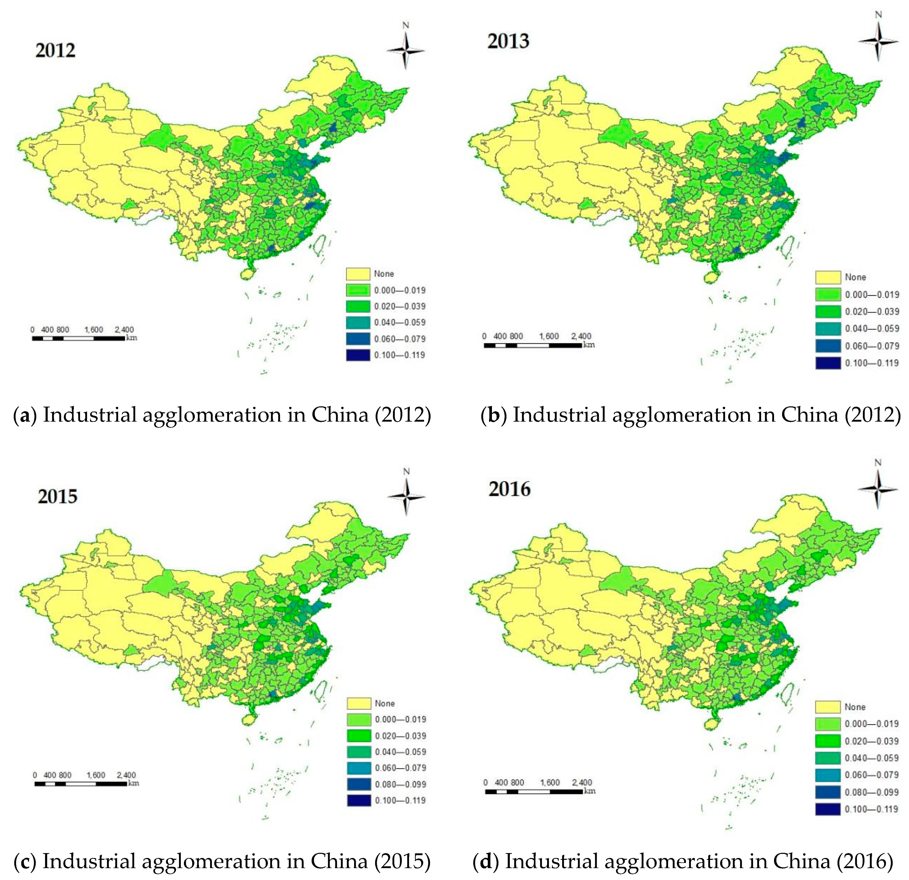
4.1.1. Spatio-Temporal Distribution of Industrial Agglomeration

Figure 1 shows that there are obvious spatial distribution characteristics of industrial agglomeration in China, which are characterised by high agglomeration in the eastern region, low agglomeration in the western region, and the highest level of industrial agglomeration in the coastal region. In addition, a clear correlation can be found between the level of industrial agglomeration in cities and their level of economic development. The exceptions to this are Beijing, Shanghai, and Shenzhen. This is because these first-tier cities have moved towards an innovation-driven and sustainable development path and have shifted many industrial enterprises out of the city.

Figure 1 shows that the temporal distribution of industrial agglomeration in China has been stable. From 2012 to 2016, the spatial distribution characteristics of industrial agglomeration did not change significantly, indicating that the distribution characteristics of industrial agglomeration in China are stable, indicating that China’s industrial development pattern has formed a more complete system.

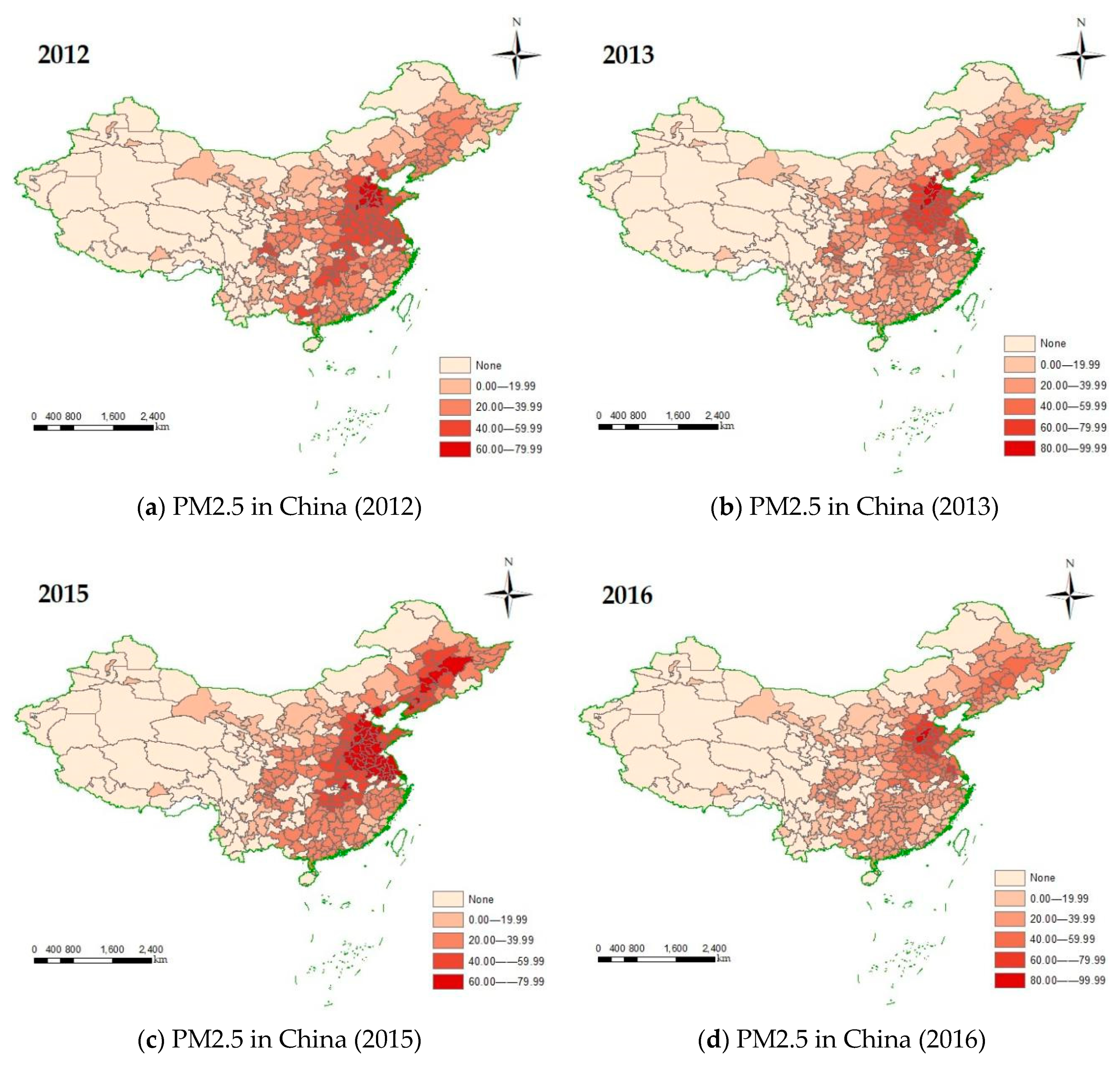
4.1.2. Spatio-Temporal Distribution of PM2.5

Figure 2 shows that there are obvious spatial distribution characteristics of PM2.5 pollution in China, and the overall pattern is similar to the distribution pattern of industrial agglomeration, specifically: PM2.5 pollution in the east and central regions (mainly in the Yangtze River Delta city cluster and the Pearl River Delta city cluster) is significantly higher than that in other regions, PM2.5 pollution in the southeast coastal region is smaller, and PM2.5 in the western and northern regions is at a very low level. The cities in Hebei Province have the highest PM2.5 pollution levels, and the PM2.5 pollution levels in its neighbouring provinces are decreasing in a radial manner. Furthermore, similar to the level of industrial agglomeration, the three first-tier cities of Beijing, Shanghai and Shenzhen have much lower PM2.5 levels than their neighbouring cities, indirectly indicating the relationship between industrial agglomeration and PM2.5.

Figure 2 shows that there is a clear temporal distribution of PM2.5 pollution in China. It can be found that the spatial pattern has not changed significantly over time, but the PM2.5 pollution levels across China show a decreasing trend year by year. Even in the urban masses of Hebei Province, where PM2.5 pollution is most serious, the number of cities meeting the highest standards of PM2.5 pollution has been decreasing.

4.2. Spatial Auto-Correlation Analysis

“Everything is related to everything else, but near things are more related than distant things” [40]. This view is known as the “first law of geography” and is one of the basic theories of spatial econometrics. The need to add spatial effects to the STIRPAT model depends on the existence of spatial auto-correlation between PM2.5 concentrations and industrial agglomeration variables at the prefecture level in China; thus it is necessary to conduct spatial auto-correlation tests on the explanatory variables PM2.5 concentrations and industrial agglomeration variables to determine their spatial distribution characteristics. If the regional PM2.5 concentration and industrial agglomeration show random distribution characteristics, then there is no need to use spatial measures; if they show spatial agglomeration characteristics, then spatial measures should be used. Since the article chooses the first-order adjacency matrix as the spatial weight matrix of the main regression model, the spatial auto-correlation analysis of regional PM2.5 concentration is carried out based on the first-order adjacency matrix.

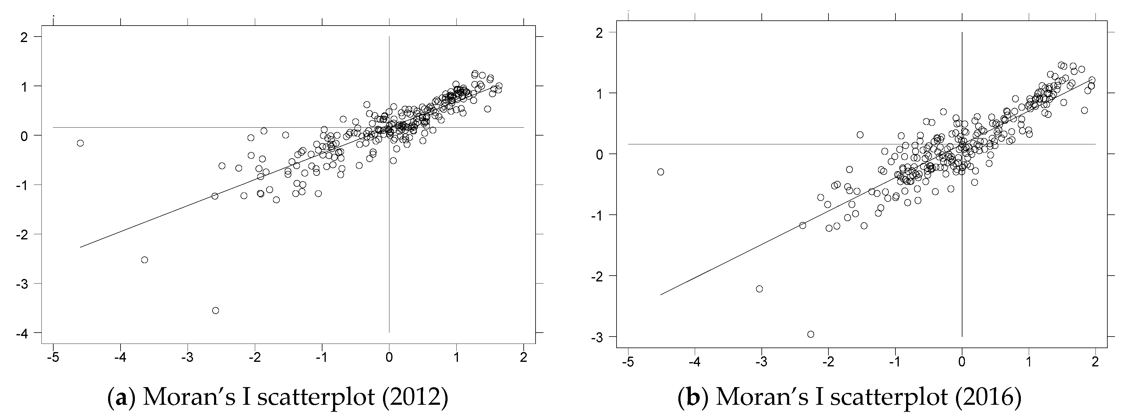
4.2.1. Global Spatial Auto-Correlation Analysis

Global spatial auto-correlation analysis examines the spatial clustering of the entire spatial sequence. The Moran’s I test is commonly used, with values in the range [–1, 1], indicating positive spatial auto-correlation when the value is greater than 0, negative spatial auto-correlation when the value is less than 0, and no spatial auto-correlation when the value is equal to 0. When the value is equal to 0, there is no spatial auto-correlation. The specific formula is as follows:

$$I=\frac{{{\displaystyle \sum }}_{i=1}^n{{\displaystyle \sum }}_{j=1}^n{w}_{ij}\left(x_i-\overline{x}\right)\left(x_j-\overline{x}\right)}{S^2{{\displaystyle \sum }}_{i=1}^n{{\displaystyle \sum }}_{j=1}^n{w}_{ij}},$$

(16)

where, $S^2=\frac{{{\displaystyle \sum }}_{i=1}^n{\left(x_i-\overline{x}\right)}^2}{n}$ is the sample variance and $w_{ij}$ is the spatial weight matrix element; n is the sample size, i.e., the number of regions under study; $x_i$ and $x_J$ denote the attribute, i.e., PM2.5 concentration, for regions i and j, respectively; and $\overline{x}=\frac{1}{n}{\displaystyle \sum }_{i=1}^n{x}_i$, i.e., the mean value of $x_i$.

Using Stata 16.1 SE, PM2.5 concentrations and industrial agglomeration data of 253 prefectural-level cities in China were selected to calculate Moran’s I index for both variables in China from 2012–2016. As shown in

Table 3. Moran’s I (2012–2016).

Panel A: ln PM
Year	Moran’s I	p-value
2012	0.174	0.000
2013	0.162	0.000
2014	0.168	0.000
2015	0.232	0.000
2016	0.194	0.000
Panel B: ln IA
Year	Moran’s I	p-value
2012	0.126	0.000
2013	0.128	0.000
2014	0.113	0.000
2015	0.135	0.000
2016	0.142	0.000

. It can be found that the Moran’s I values of PM2.5 concentration and industrial agglomeration for all years are greater than 0 and pass the 1% significance test, indicating that there is a significant positive spatial auto-correlation and a significant spatial dependence between PM2.5 concentration and industrial agglomeration in China, and therefore it is necessary to further investigate the relationship between industrial agglomeration and PM2.5 concentration using a spatial Durbin model.

4.2.2. Local Spatial Auto-Correlation Analysis

The Moran’s I index reveals the global spatial correlation of regional haze concentrations, while the Moran’s I scatterplot is used to depict local spatial correlations, thus illustrating the spatial clustering of high (or low) observations of haze concentrations. Moran’s I scatterplot is based on a standardised Cartesian coordinate system, with the horizontal coordinate representing the attributes of the region and the vertical coordinate representing the mean of the attributes of neighbouring regions, while the Moran’s I index mentioned above can be considered as the slope of the regression line of the scatterplot. In the four quadrants of the Moran’s I scatterplot, each quadrant represents a different spatially correlated state. The meaning of spatial correlation in each of the four quadrants is: (1) in the upper right quadrant, it represents areas with high PM2.5 concentrations and adjacent areas with high PM2.5 concentrations, i.e., high values are spatially correlated with high values; (2) in the lower left quadrant, it represents areas with low PM2.5 concentrations and adjacent areas with low PM2.5 concentrations, i.e., low values are spatially correlated with low values; (3) in the lower right quadrant, it represents areas with high PM2.5 concentrations whose neighbouring areas have low PM2.5 concentrations, i.e., a spatial correlation between high and low values; (4) in the upper left quadrant, it represents areas with low PM2.5 concentrations whose neighbouring areas have high PM2.5 concentrations, i.e., a spatial correlation between low and high values.

This paper plots the Moran’s I scatterplot from 2012 to 2016, but as the distribution of the scatterplot does not change significantly with increasing years, this paper only shows the Moran’s I scatterplot for 2012 and 2016, as shown in Figure 3. An overview of all regions reveals that: (1) The spatial clustering distribution of regional PM2.5 concentrations in China is stable, mostly in the upper right quadrant and lower left quadrant, showing positive spatial correlation, which indicates that PM2.5 concentrations in each region are clustered in spatial distribution (spatial dependence) and also reflects the variability of PM2.5 concentrations in general (spatial heterogeneity). (2) The scatter density in the upper right quadrant decreases as the year increases, with a number of areas moving from the upper right quadrant to the lower left quadrant, i.e., from areas of concentration of high and high values to areas of concentration of low and low values. This indicates a decrease in haze concentrations in China’s prefecture-level cities from 2012 to 2016.

4.3. Further Improvement of Empirical Model

4.3.1. Panel Model Effects Test

Panel models come in various forms and can usually be classified as: mixed regression models, fixed-effects models, and random-effects models. The specificity of panel data for prefecture-level cities has led to the use of fixed-effects models. However, there are three forms of fixed-effects models: spatial fixed effects, time fixed effects, and two-way fixed effects. In order to select the appropriate form of panel model, this paper uses the Durbin–Wu–Hausman test to see whether the model should use fixed effects. As the model is estimated using the great likelihood method, the likelihood ratio test (LR) is used to determine exactly which fixed-effects model should be used in this paper.

Table 4. Panel effect test.

Hypothesis	LR	Durbin–Wu–Hausman
Hypothesis: Time fixed effect nested in two-way fixed effect	3448.00 ***	103.67 ***
Hypothesis: Individual fixed effect nested in two-way fixed effect	43.33 ***

*** indicate statistical significance at the 1% level.

shows the results of the LR test and the Durbin–Wu–Hausman test. The Durbin–Wu–Hausman coefficient is significant at the 1% level, indicating that a fixed-effects model should be used in this paper. Both results of the LR test reject the original hypothesis at the 1% level, and therefore, a two-way fixed-effects model should be used in this paper.

4.3.2. Spatial Model Effects Tests

Starting with a spatial Durbin model for modelling analysis of spatial econometric models may be a good option, but a series of spatial correlation tests are needed to confirm which spatial econometric model is more effective in explaining the data. (i) We use the classical LM test and the robust LM test to test both whether a spatial lag model or a spatial error model is more appropriate to describe the data relative to the OLS model [55]. (ii) If the OLS model is rejected in favour of the spatial lag model or the spatial error model, the spatial Durbin model should be used for estimation. As the model is estimated using the great likelihood method, the likelihood ratio test (LR) is used in this paper to select the model to determine whether the spatial Durbin model can be reduced to a spatial lag model and a spatial error model.

The results of the LM and LR tests are shown in

Table 5. Spatial panel model test.

Hypothesis	LM	Robust-LM	Hypothesis	LR
Null hypothesis: SEM is not better than OLS model	2406.781 ***	2396.70 ***	Null hypothesis: SDM can be simplified to SEM	13.92 **
Alternative hypothesis: SEM is better than OLS model			Alternative hypothesis: SDM cannot be simplified to SEM
Null hypothesis: SLM is not better than OLS model	12.667 ***	2.587	Null hypothesis: SDM can be simplified to SLM	26.81 ***
Alternative hypothesis: SLM is better than OLS model			Alternative hypothesis: SDM cannot be simplified to SLM

***, ** respectively, indicate statistical significance at the 1% and 5% levels.

. In both the LM test and the robust LM test, most of the LM values passed the 1% significance test, rejecting the original hypothesis and indicating that the spatial model outperforms the OLS model; in the LR test, the LR values passed the 5% and 1% significance tests, respectively, indicating that the spatial Durbin model (SDM) could not be simplified to the spatial lag model (SLM) or the spatial error model (SEM). Therefore, SDM is the most suitable spatial model for this paper.

4.4. Spatial Econometric Analysis

4.4.1. Estimated Results of the Spatial Econometric Model

In this paper, the model of Equation (10) was operated using maximum likelihood estimation based on annual panel data of 253 prefecture-level cities in China from 2012–2016 using Stata 16.1 SE. To test the robustness of the regression results, we gradually added control variables to the regression process of SDM, and the final regression results are shown in

Table 6. Comparison results of spatial Durbin model.

Variable	(1)	(2)	(3)	(4)	(5)
IA	−0.1669 *** (−10.46)	−0.1386 *** (−7.51)	−0.1403 *** (−7.53)	−0. 1198 *** (−6.12)	−0.1124 *** (−5.67)
W*IA	0.3701 *** (3.74)	0.4452 *** (3.34)	0.4559 *** (3.37)	0. 4754 *** (3.49)	0. 4381 *** (3.17)
GDP		−0.0887 *** (−3.02)	−0.0817 *** (−2.72)	−0. 0693 ** (−2.30)	−0.0770 ** (−2.55)
W*GDP		0.0362 (0.69)	0.1946 * (1.67)	0.2921 * (1.91)	0.3412 ** (2.21)
TRA			−0.0053 (−0.70)	−0.0064 (−0.86)	−0.0065 (−0.86)
W*TRA			0.0509 * (1.71)	0. 0583 * (1.95)	0. 0521 * (1.72)
TEC				−0.0308 *** (−3.26)	−0.0294 *** (−3.12)
W*TEC				−0.0387 (−0.60)	−0. 0149 (−0.22)
POP					−0.2049 ** (−2.39)
W*POP					−1.0508 (−1.31)
R2	0.1679	0.2245	0.2451	0.2560	0.2768
Spat-rho	0.8125 *** (16.77)	0.7866 *** (14.18)	0.7613 *** (12.64)	0. 7614 *** (12.61)	0.7475 *** (12.03)
Log-L	1094.5435	1099.7333	1101.2793	1106.7502	1110.3296

*, **, and *** indicate statistical significance at the 10%, 5%, and 1% levels, respectively. Z statistics in parentheses.

. Column 1 is the regression result including only the independent variable IA and its spatial lag term, while column 5 is the regression result including all control variables and their spatial lag terms. We found that the coefficient of IA is always negatively significant at the 1% level when the control variables are gradually added, suggesting that industrial agglomeration suppresses the level of local haze pollution. The coefficient of W*IA is always positively significant at the 1% level, suggesting that industrial agglomeration increases the level of haze pollution in the surrounding area. However, Elhorst pointed out that the regression coefficients of SDM do not have explanatory power and it is meaningless to discuss the values and significance of their coefficients. He emphasised that the coefficients should be decomposed into direct and indirect effects before the regression results are interpreted. [56] Therefore, the empirical results in Table 6 merely demonstrate that the results are robust and provide some evidence for our conclusions. Further, the paper decomposes the coefficients of the independent variables to obtain direct and indirect effects, as shown in

Table 7. Direct and indirect effects.

Direct Effect	Coefficient	Z-Value	p-Value	Indirect Effect	Coefficient	Z-Value	p-Value
IA	−0.105	−5.10	0.000	IA	1.400	3.06	0.002
GDP	−0.073	−2.42	0.016	GDP	1.165	1.49	0.137
TRA	−0.004	−0.66	0.507	TRA	0.186	1.34	0.181
TEC	−0.030	−3.13	0.002	TEC	−0.158	−0.50	0.614
POP	−0.227	−2.67	0.007	POP	−4.966	−1.37	0.172

.

Based on the spatial Durbin model (SDM) partial differential method to decompose the spillover effects, the total effect can be decomposed into two parts: one is the direct effect, which indicates the impact of local industrial agglomeration on local haze pollution; the other is the indirect effect, also known as the spillover effect, which indicates the impact of local industrial agglomeration on haze pollution in neighbouring areas. According to the decomposition results in Table 7, (i) the coefficient of industrial agglomeration under the direct effect is −0.105 and is significant at the 1% level, which means that an increase in the scale of local industrial agglomeration will lead to a decrease in local haze pollution; (ii) the coefficient of industrial agglomeration under the indirect effect is 1.400 and is significant at the 1% level, which means that an increase in the scale of local industrial agglomeration will lead to an increase in haze pollution in neighbouring areas. It can be seen that there is a significant spatial spillover effect of industrial agglomeration, and the inter-regional spillover is greater than the intra-regional spillover.

4.4.2. Conclusion Analysis and Explanation

In the context of China’s reality, the possible reasons are as follows:

• Local industrial agglomeration creates economies of scale, brings advanced technology to the local area, promotes the upgrading of local industry [3], improves the energy-saving and emission reduction capabilities of industrial enterprises [6], and develops towards an environment-friendly and clean green economy [12]. The positive externalities brought about by agglomeration, such as reduced transport and information communication costs (labour and technology spillover effects) between enterprises [43], have led to an increase in the overall economic productivity of local enterprises, improved energy efficiency, and reduced pollutant emissions [57], thus improving the efficiency of the green economy in the region [58]. Therefore, the expansion of local industrial agglomeration is beneficial to the control of haze and reduces the concentration of PM2.5 [59].
• Due to the mobility of technology, capital, and talent, when the scale of local industrial agglomeration rises and industrial density becomes too high, the local workforce cannot keep up with the demand for efficient production [2], and thus local enterprises recruit more labour from neighbouring areas and attract more talent, creating a “siphon effect” on neighbouring cities [3]. As a result, technology, capital, and talent will inevitably move to cities with high levels of industrial development, further increasing the technological gap between local and neighbouring areas [60]. At this point, the negative externalities of industrial agglomeration on neighbouring regions are greater than the positive externalities, which is not conducive to neighbouring cities improving their technology and developing a green economy [61]. In addition, due to the existence of promotion tournaments between regional governments in China, when the scale of local industrial agglomeration rises, neighbouring regions are forced to increase their industrial development due to promotion pressure [62], seeking regional economic development and forming inter-regional industrial level competition. However, due to the inadequate technology level of the neighbouring regions, they cannot form economies of scale like the regions with high industrial agglomeration scale [63], making the development of industry in the neighbouring regions instead increase the level of haze pollution.

5. Discussion

Some studies believe that an important reason for the spatial dependence of haze pollution is industrial agglomeration and point out that with the growth of GDP, the degree of haze pollution will continue to rise [6,7]. Therefore, industrial agglomeration not only promotes regional economic growth and development but also leads to many environmental problems that cannot be ignored. Britain and the United States caused serious haze to the country’s environment during the great development. As a developing country, China’s industrial agglomeration areas have low production efficiency, poor industrial relevance, and lack of innovation ability, which leads to the pollution spillover effect of industrial agglomeration areas, especially in the northeast, which is a heavy industry area. This requires that all regions in China actively explore the innovation of industrial science and technology, enhance the industrial value chain, and form a development mode of energy conservation and environmental protection.

This paper provides some enlightenment for thinking about the differences in haze pollution in different regions of China. Being similar to the research [3,42], this study concludes that industrial agglomeration has a negative external effect on haze pollution and will cause the deterioration of the ecological environment. There is much literature on industrial agglomeration and environmental pollution, but few studies related to haze pollution. Therefore, this paper brings industrial agglomeration and haze pollution into the framework to investigate the internal relationship between industrial agglomeration and haze pollution. Most previous studies on industrial agglomeration took provinces as the unit and did not subdivide urban areas. This study took Chinese cities as the research objects to investigate the impact of industrial agglomeration within cities on haze pollution. Considering the spatial spillover effect of industrial agglomeration and haze pollution, this paper uses a spatial econometric model to test the external effect of industrial agglomeration, and analyses the direct impact of industrial agglomeration on haze pollution in different urban areas and the spatial spillover impact on haze pollution in neighbouring urban areas. At the same time, some parts of this study need to be improved in the future.

5.1. Robustness Test Using Inverse-Distance Matrix and Economic Geography Nested Matrix

To ensure the robustness of the conclusions, the paper will further replace the adjacency matrix and re-substitute it into the spatial Durbin model for empirical evidence. In this paper, the same partial differential decomposition of the spillover effects of industrial agglomeration is done, and the direct and indirect effects of industrial agglomeration are shown in

Table 8. Inverse-distance-based spatial weights matrix.

Direct Effect	Coefficient	Z-Value	p-Value	Indirect Effect	Coefficient	Z-Value	p-Value
IA	−0.099	−4.50	0.000	IA	0.213	2.42	0.015
GDP	−0.063	−2.06	0.040	GDP	−0.109	−0.84	0.399
TRA	−0.009	−1.20	0.229	TRA	−0.017	−0.60	0.548
TEC	−0.022	−2.07	0.039	TEC	0.059	1.21	0.227
POP	−0.196	−2.12	0.034	POP	−0.611	−1.05	0.296

and

Table 9. Nested Weights Matrix.

Direct Effect	Coefficient	Z-Value	p-Value	Indirect Effect	Coefficient	Z-Value	p-Value
IA	−0.095	−4.31	0.000	IA	0.186	1.86	0.063
GDP	−0.066	−2.16	0.031	GDP	−0.033	−0.24	0.811
TRA	−0.006	−0.92	0.358	TRA	−0.014	−0.50	0.616
TEC	−0.023	−2.21	0.027	TEC	0.024	0.50	0.618
POP	−0.188	−2.04	0.041	POP	−0.204	−0.30	0.763

.

The direct and indirect effects of industrial agglomeration are shown in Table 8 and Table 9: the signs of the coefficients of the variables in the direct and indirect effects are the same, and the significance is approximately the same. Both the direct effect of the IA term and its indirect effect are significant. Overall, the empirical results are consistent with the previous paper, indicating that the previous conclusions are robust.

5.2. Discussion on Endogeneity Based on GS2SLS

The previous regression results suggest that high levels of industrial agglomeration can reduce local haze pollution; however, areas with low levels of haze pollution may attract more industrial presence due to low environmental regulation, leading to reverse causality in the empirical model. Therefore, this paper employs both two-stage least squares regression and Generalized Spatial Two-stage Least Square, using topographic relief (RDLS) as an instrumental variable for the explanatory variable industrial agglomeration (IA).

Topographic relief is one of the most important factors affecting population distribution and labour intensity in China. The topographic relief of a region is determined by the combination of the highest and lowest elevation, the flat land area, and the total area of the region and is a naturally occurring and geographically objective factor. It can therefore be assumed that this indicator does not directly affect the level of haze pollution. Topographic relief, however, affects population inflow and thus negatively influences the degree of industrial agglomeration. It is therefore reasonable to use topographic relief as an instrumental variable for industrial agglomeration. Using GIS technology and China’s 1:1 million geographic digital elevation simulation data, raster data were extracted based on a 1 km × 1 km specification, and a 10 km × 10 km raster was selected as the measurement unit. Within each measurement unit (100 km²), the relief degree of terrain (RDLS) was measured using the formula:

$$RDLS=\frac{[\max (H)-\min (H)]\times [1-P(A)/A]}{500},$$

(17)

where max(H) and min(H) are the maximum and minimum elevation within each measurement unit, A is the area of the measurement unit, and P(A) is the area of flat land within the measurement unit, where the difference between the maximum and minimum elevation within 25 km² is less than or equal to 30 m.

Columns 1–2 of

Table 10. Direct and indirect effects.

Variable	2SLS		GS2SLS
	(1)	(2)	(3)	(4)	(5)
	Stage I	Stage II	Results	Direct Effect	Indirect Effect
RDLS	−0.1903 *** (−11.53)
IA		−2.0973 *** (−12.23)	−2.1510 *** (−5.01)	−2.0071 *** (−4.42)	2.7075 *** (3.50)
GDP	1.2089 *** (34.70)	−2.5677 *** (−11.22)	−2.6906 *** (−4.52)	−2.5340 *** (−4.18)	2.9479 *** (3.08)
TRA	0.0682 *** (4.44)	−0.1319 *** (−4.09)	0.0121 (0.14)	0.0266 (0.33)	0.2736 (0.68)
TEC	0.0857 *** (4.84)	−0.1580 *** (−4.20)	−0.2570 *** (−3.04)	−0.2242 ** (−2.49)	0.6174 * (1.96)
POP	0.8425 *** (30.44)	−1.5616 *** (−9.35)	−1.6410 *** (−3.80)	−1.5681 *** (−3.69)	1.3715 ** (2.32)
Constant	−23.88 *** (−64.51)	52.64 *** (12.08)	29.85 (1.16)
R2	0.8337		0.2110
F	1262.73
Minimum eigenvalue	132.866	10%, 16.38
N	1265	1265	1265	1265	1265

*, **, and *** indicate statistical significance at the 10%, 5%, and 1% levels, respectively.

present the results of the estimation using the instrumental variable 2sls, and Columns 3–5 show the results using the instrumental variable Generalized Spatial Two-stage Least Square. To test the plausibility of the instrumental variables, the F-test of the Cragg–Donald Wald rank test is adopted in this paper. The original hypothesis is that the relationship between the instrumental variables and the endogenous variables is weak. As a rule of thumb, an F-value greater than 10 rejects the original hypothesis. Therefore, the instrumental variables are strongly correlated with the endogenous variables in this paper. The minimum eigenvalue test statistic of 132.866 is greater than the critical value of 16.38, indicating that there is no weak instrumental variable problem.

Column 1 of Table 10 shows the results of the first stage of the 2SLS regression, and it can be seen that topographic relief (RDLS) and industrial agglomeration (IA) are negatively correlated. This is due to the fact that areas with high topographic relief are more difficult for population inflows and outflows and thus more difficult for industrial agglomeration effects to develop. Column 1 shows the regression results after controlling for the endogeneity between industrial agglomeration and haze using topographic relief. The regression results show that the coefficient of IA is significantly negative at the 1% level, indicating that industrial agglomeration suppresses local haze pollution levels. Column 3 considers both the endogeneity and spatial spillover effects between industrial agglomeration and haze. After considering the spatial spillover effect, the coefficient of IA is still significantly negative at the 1% level, but the effect of industrial agglomeration on the surrounding area cannot be observed. Columns 4–5 decompose the effect of industrial agglomeration on haze into a direct effect and an indirect effect. The results show that the direct effect of industrial agglomeration on haze is significantly negative, i.e., industrial agglomeration has a suppressive effect on local haze pollution. At the same time, the indirect effect of industrial agglomeration on haze is significantly positive, which indicates that industrial agglomeration exacerbates the haze pollution in the surrounding areas. This is consistent with the main regression results. It can be argued that its empirical results remain robust after the endogeneity of this paper has been treated using instrumental variables.

5.3. Limitations and Future Research

We believe that although we achieved the objectives of this paper to a certain extent, there are still some shortcomings and areas for future improvement:

• Using spatial econometrics as an analytical tool, this paper extends the study to 253 prefecture-level cities. To a certain extent, it alleviates the endogeneity implications of the lack of freedom in previous studies and the neglect of the causal identification problem, e.g., [3,26]. The possible endogeneity problems due to insufficient causal identification are also discussed. However, due to the difficulty of obtaining data and the limitations of the development of spatial econometrics, the scientific tools for the discussion of the endogeneity problem are still relatively homogeneous. With the introduction of new spatial econometric causal inference methods, further improvements to the study will be made.
• In the baseline regression and robustness tests, three spatial weight matrices are used to discuss the problem, which to some extent ameliorates the problem of unrobustness in previous studies. However, the reasonableness of the choice of spatial weight matrix has been a major problem in such studies. We will also follow up on related studies and improve on them.
• For the reasons of the results, due to the consideration of space and other factors, this paper mainly adopts a qualitative research method based on the combination of previous literature. In subsequent studies, we will try to discuss the mechanism issue in detail empirically.

6. Conclusions and Policy Implications

Economic factors are easily ignored in sustainable urban development. The highlight of this paper is the exploration of whether economic factors can be compatible with environmental factors. Specifically, based on data related to 253 prefecture-level cities in 30 provincial administrative units in China from 2012–2016, this paper uses spatial measurement as a tool to explore whether industrial agglomeration should exist in sustainable cities from the perspective of haze pollution prevention and control and further analyses the spatial heterogeneity and spatial spillover effects of pollution reduction effects of industrial agglomeration.

This study found that there is an obvious positive spatial correlation between industrial agglomeration and haze pollution, and the strong and weak agglomeration has been stable in the past five years, with a typical High–High and Low–Low divergence phenomenon. In other words, haze pollution in China is clustered in terms of spatial distribution and spatially heterogeneous in terms of concentration. However, there is a tendency to move from areas of concentration of High–High values to areas of concentration of Low–Low values over time, indicating a decrease in haze concentrations in Chinese prefecture-level cities from 2012 to 2016.

SDM with spatial and time-period fixed effects is used to regress industrial agglomeration and haze pollution. The regression results show that an increase in the scale of local industrial agglomeration leads to a decrease in local haze pollution; however, an increase in the scale of local industrial agglomeration leads to an increase in haze pollution in neighbouring areas. There is a significant spatial spillover effect of industrial agglomeration, with spatial heterogeneity and the inter-regional spillover being greater than the intra-regional spillover.

This paper will further use the inverse-distance matrix and economic geography nested matrix to replace the adjacency matrix and re-substitute into the spatial Durbin model for empirical research. The results of the robustness test show that the signs of the coefficients of the variables in the direct effect and the indirect effect are consistent and approximately the same in terms of significance. In particular, both the direct effect of the IA term and its indirect effect are significant, and overall, this empirical result is consistent with the baseline study. The empirical results remain robust after the instrumental variables are used to treat the endogeneity of this paper.

In sustainable urban planning, the spatial distribution of industrial enterprises is rationalised, rather than simply shifting polluting enterprises away from the region. The findings of this paper suggest that high-intensity industrial agglomeration is conducive to the reduction of haze pollution, suggesting that economic development and environmental protection may lead to a “double-win” path.

Performance evaluation policies for industrial development, especially environmental evaluation policies, should reflect regional synergy. The findings of this paper show that the increase in the level of regional industrial agglomeration produces negative externalities on haze pollution in other cities. Therefore, when evaluating the performance of environmental protection in regional economic development, isolated assessments should be avoided and an overall regional performance assessment can be conducted to avoid malicious competition between regional officials, which increases this negative externality.

In the construction of urban agglomerations, the “siphoning effect” should be avoided, and the coordinated development of regional industries should be achieved. The results of this study show that the negative impact of industrial agglomeration in the region on other regions is mainly due to the “siphon effect”. Therefore, industrial policies should be reasonably arranged and planned to avoid excessive competition and factor congestion. While forming large urban agglomerations, the surrounding small and medium-sized cities should not be turned into “industrial graveyards”.

Green transformation of traditional manufacturing industries and establishment of a green, low-carbon, and circular development system: The results of this study show that improving the efficiency of the manufacturing industry can indeed improve haze pollution, accelerate the development of advanced manufacturing industries, support green and clean production, promote the green transformation of traditional manufacturing industries, and establish a green low-carbon recycling development system. On the one hand, encourage the separation of the manufacturing industry, actively develop the service industry, vigorously guide the development of productive services in the direction of specialisation and socialisation, and cultivate a number of specialised service enterprises with strong competitive ability and high level of research and development; on the other hand, continuously expand the length of the industrial chain of manufacturing industry synergistic agglomeration, manufacturing efficiency, and haze pollution industry, and enhance such high-end value chain as research and development design, engineering management, financial leasing, equipment testing the design of the ring, and more service elements into the final product to enhance the level of industry chain services and product added value.

References

1. Zhu, X.T.; Ye, C.; Li, S.M. Research progress of sustainable cities and its implications for national territory spatial plan. J. Nat. Resour. 2020, 35, 2120–2133. [Google Scholar]
2. Li, Y.; Tang, Y.; Wang, K.; Zhao, Q. Environmental Regulation and China’s Regional Innovation Output—Empirical Research Based on Spatial Durbin Model. Sustainability 2019, 11, 5602. [Google Scholar] [CrossRef]
3. Zhao, H.; Cao, X.; Ma, T. A spatial econometric empirical research on the impact of industrial agglomeration on haze pollution in China. Air Qual. Atmos. Health 2020, 13, 1305–1313. [Google Scholar] [CrossRef]
4. Wang, K.; Tang, Y.; Chen, Y.; Shang, L.; Ji, X.; Yao, M.; Wang, P. The Coupling and Coordinated Development from Urban Land Using Benefits and Urbanization Level: Case Study from Fujian Province (China). Int. J. Environ. Res. Public Health 2020, 17, 5647. [Google Scholar] [CrossRef] [PubMed]
5. Guan, X.; Wei, H.; Lu, S.; Dai, Q.; Su, H. Assessment on the urbanization strategy in China: Achievements, challenges and reflections. Habitat Int. 2018, 71, 97–109. [Google Scholar] [CrossRef]
6. Guo, Y.; Tong, L.; Mei, L. The effect of industrial agglomeration on green development efficiency in Northeast China since the revitalization. J. Clean. Prod. 2020, 258, 120584. [Google Scholar] [CrossRef]
7. Chen, W.; Lei, Y.; Wu, S.; Li, L. Opportunities for low-carbon socioeconomic transition during the revitalization of Northeast China: Insights from Heilongjiang province. Sci. Total Environ. 2019, 683, 380–388. [Google Scholar] [CrossRef]
8. Lin, W.L.; Chen, T.P. China’s widening economic disparities and its ‘Go West Program’. J. Contemp. China 2004, 13, 663–666. [Google Scholar] [CrossRef]
9. Liu, H.; Wang, Y.; Jiang, J.; Wu, P. How green is the “Belt and Road Initiative”?—Evidence from Chinese OFDI in the energy sector. Energy Policy 2020, 145, 1117. [Google Scholar] [CrossRef]
10. Zeng, D.; Zhao, L. Pollution havens and industrial agglomeration. J. Environ. Econ. Manag. 2009, 58, 141–153. [Google Scholar] [CrossRef] [Green Version]
11. Porter, M.E. Towards a dynamic theory of strategy. Strat. Manag. J. 1991, 12, 95–117. [Google Scholar] [CrossRef]
12. Kesidou, E.; Wu, L. Stringency of environmental regulation and eco-innovation: Evidence from the eleventh Five-Year Plan and green patents. Econ. Lett. 2020, 190, 109090. [Google Scholar] [CrossRef]
13. Wang, X.; Klemeš, J.J.; Dong, X.; Fan, W.; Xu, Z.; Wang, Y.; Varbanov, P.S. Air pollution terrain nexus: A review considering energy generation and consumption. Renew. Sustain. Energy Rev. 2019, 105, 71–85. [Google Scholar] [CrossRef]
14. Tang, Y.; Chen, Y.; Wang, K.; Xu, H.; Yi, X. An Analysis on the Spatial Effect of Absorptive Capacity on Regional Innovation Ability Based on Empirical Research in China. Sustainability 2020, 12, 3021. [Google Scholar] [CrossRef] [Green Version]
15. Cavaco, S.; Crifo, P. CSR and financial performance: Complementarity between environmental, social and business behaviours. Appl. Econ. 2014, 46, 3323–3333. [Google Scholar] [CrossRef]
16. Javorcik, B.S.; Wei, S.J. Pollution Havens and Foreign Direct Investment: Dirty Secret or Popular Myth? Contrib. Econ. Anal. Policy 2005, 3, 12. [Google Scholar] [CrossRef] [Green Version]
17. Yao, M.; Zhang, Y. Evaluation and Optimization of Urban Land-Use Efficiency: A Case Study in Sichuan Province of China. Sustainability 2021, 13, 1771. [Google Scholar] [CrossRef]
18. Tsai, K.; Yang, S. Firm innovativeness and business performance: The joint moderating effects of market turbulence and competition. Ind. Mark. Manag. 2013, 42, 1279–1294. [Google Scholar] [CrossRef]
19. Singh, J.; Gupta, P.; Gupta, D.; Verma, S.; Prakash, D.; Payra, S. Fine particulate pollution and ambient air quality: A case study over an urban site in Delhi, India. J. Earth Syst. Sci. 2020, 129, 1–15. [Google Scholar] [CrossRef]
20. Chen, C.; Sun, Y.; Lan, Q.; Jiang, F. Impacts of industrial agglomeration on pollution and ecological efficiency-A spatial econometric analysis based on a big panel dataset of China’s 259 cities. J. Clean. Prod. 2020, 258, 120721. [Google Scholar] [CrossRef]
21. Zhu, X.; Zeng, A.; Zhong, M.; Huang, J.; Qu, H. Multiple impacts of environmental regulation on the steel industry in China: A recursive dynamic steel industry chain CGE analysis. J. Clean. Prod. 2019, 210, 490–504. [Google Scholar] [CrossRef]
22. Levinson, A.; Taylor, M.S. Unmasking the Pollution Haven Effect. Int. Econ. Rev. 2010, 49, 223–254. [Google Scholar] [CrossRef] [Green Version]
23. Bu, M.; Liu, Z.; Wagner, M.; Yu, X. Corporate social responsibility and the pollution haven hypothesis: Evidence from multinationals’ investment decision in China. Asia-Pac. J. Account. Econ. 2013, 20, 85–99. [Google Scholar] [CrossRef]
24. Tao, F.; Zhao, J.; Zhou, H. Does Environmental Regulation Improve the Quantity and Quality of Green Innovation: Evidence from the Target Responsibility System of Environmental Protection. China Ind. Econ. 2021, 2, 136–154. [Google Scholar] [CrossRef]
25. Lin, Y.; Zou, J.; Wei, Y.; Li, C.Q. A Review of Recent Advances in Research on PM5 in China. Int. J. Environ. Res. Public Health 2018, 15, 438. [Google Scholar] [CrossRef] [Green Version]
26. Ethan, C.J.; Mokoena, K.; Yu, Y.; Shale, K.; Fan, Y.; Rong, J.; Liu, F. Association between PM2.5 and mortality of stomach and colorectal cancer in Xi’an: A time-series study. Environ. Sci. Pollut. Res. 2020, 27, 22353–22363. [Google Scholar] [CrossRef]
27. Monks, P.; Granier, C.; Fuzzi, S.; Stohl, A.; Williams, M.; Akimoto, H.; Amann, M.; Baklanov, A.; Baltensperger, U.; Bey, I.; et al. Atmospheric composition change—Global and regional air quality. Atmos. Environ. 2009, 43, 5268–5350. [Google Scholar]
28. Liu, X.; Zou, B.; Feng, H.; Liu, N.; Zhang, H. Anthropogenic factors of PM5 distributions in China’s major urban agglomerations: A spatial-temporal analysis. J. Clean Prod. 2020, 264, 1217. [Google Scholar] [CrossRef]
29. Askariyeh, M.H.; Venugopal, M.; Khreis, H.; Birt, A.; Zietsman, J. Near-Road Traffic-Related Air Pollution: Resuspended PM2.5 from Highways and Arterials. Int. J. Environ. Res. Public Health 2020, 17, 2851. [Google Scholar] [CrossRef] [PubMed]
30. Li, H.; Lu, J.; Li, B. Does pollution-intensive industrial agglomeration increase residents’ health expenditure? Sustain. Cities Soc. 2020, 56, 10–20. [Google Scholar] [CrossRef]
31. Yun, X.; Shen, G.; Shen, H.; Meng, W.; Chen, Y.; Xu, H.; Ren, Y.; Zhong, Q.; Du, W.; Ma, J.; et al. Residential solid fuel emissions contribute significantly to air pollution and associated health impacts in China. Sci. Adv. 2020, 6, eaba7621. [Google Scholar] [CrossRef]
32. Reizer, M.; Juda-Rezler, K. Explaining the high PM10 concentrations observed in Polish urban areas. Air Qual. Atmos. Health 2015, 9, 517–531. [Google Scholar] [CrossRef] [PubMed]
33. Liu, S.; Zhu, Y.; Du, K. The impact of industrial agglomeration on industrial pollutant emission: Evidence from China under New Normal. Clean Technol. Environ. Policy 2017, 19, 2327–2334. [Google Scholar] [CrossRef]
34. Kyriakopoulou, E.; Xepapadeas, A. Atmospheric pollution in rapidly growing industrial cities: Spatial policies and land use patterns. J. Econ. Geogr. 2016. [Google Scholar] [CrossRef]
35. Czechowski, P.O.; Dąbrowiecki, P.; Oniszczuk-Jastrząbek, A.; Bielawska, M.; Czermański, E.; Owczarek, T.; Rogula-Kopiec, P.; Badyda, A. A Preliminary Attempt at the Identification and Financial Estimation of the Negative Health Effects of Urban and Industrial Air Pollution Based on the Agglomeration of Gdańsk. Sustainability 2019, 12, 42. [Google Scholar] [CrossRef] [Green Version]
36. Ciccone, A.; Hall, R.E. Productivity and the Density of Economic Activity. Am. Econ. Rev. 1996, 86, 54–70. [Google Scholar]
37. Yu, Y. CHINA_SPATDWM: Stata Module to Provide Spatial Distance Matrices for Chinese Provinces and Cities; Statistical Software Components; CORE: Bucks, UK, 2009. [Google Scholar]
38. Wang, S.K. The type and selection of weight matrix in spatial econometric model. J. Econ. Math. 2013, 30, 57–63. [Google Scholar]
39. Getis, A. Spatial weights matrices. Geogr. Anal. 2009, 41, 404–410. [Google Scholar] [CrossRef]
40. Tobler, W.R. A Computer Movie Simulating Urban Growth in the Detroit Region. Econ. Geogr. 1970, 46, 234. [Google Scholar] [CrossRef]
41. Van Donkelaar, A.; Martin, R.V.; Brauer, M.; Boys, B.L. Use of Satellite Observations for Long-Term Exposure Assessment of Global Concentrations of Fine Particulate Matter. Environ. Health Perspect. 2015, 123, 135–143. [Google Scholar] [CrossRef] [Green Version]
42. Liu, N.; Zou, B.; Feng, H.; Wang, W.; Tang, Y.; Liang, Y. Evaluation and comparison of multiangle implementation of the atmospheric correction algorithm, Dark Target, and Deep Blue aerosol products over China. Atmos. Chem. Phys. Discuss. 2019, 19, 8243–8268. [Google Scholar] [CrossRef] [Green Version]
43. Krugman, P. Increasing Returns and Economic Geography. J. Political Econ. 1991, 99, 483–499. [Google Scholar] [CrossRef]
44. Ellison, G.; Glaeser, E.L. Geographic Concentration in U.S. Manufacturing Industries: A Dartboard Approach. J. Political Econ. 1997, 105, 889–927. [Google Scholar] [CrossRef] [Green Version]
45. Wu, J.; Zheng, H.; Zhe, F.; Xie, W.; Song, J. Study on the relationship between urbanization and fine particulate matter (PM2.5) concentration and its implication in China. J. Clean Prod. 2018, 182, 872–882. [Google Scholar] [CrossRef]
46. Shen, H.; Tao, S.; Chen, Y.; Ciais, P.; Güneralp, B.; Ru, M.; Zhong, Q.; Yun, X.; Zhu, X.; Huang, T.; et al. Urbanization-induced population migration has reduced ambient PM2.5 concentrations in China. Sci. Adv. 2017, 3, e1700300. [Google Scholar] [CrossRef] [Green Version]
47. Ding, Y.; Zhang, M.; Qian, X.; Li, C.; Chen, S.; Wang, W. Using the geographical detector technique to explore the impact of socioeconomic factors on PM2.5 concentrations in China. J. Clean. Prod. 2019, 211, 1480–1490. [Google Scholar] [CrossRef]
48. Ji, S.; Cherry, C.R.; Zhou, W.; Sawhney, R.; Wu, Y.; Cai, S.; Wang, S.; Marshall, J.D. Environmental Justice Aspects of Exposure to PM2.5 Emissions from Electric Vehicle Use in China. Environ. Sci. Technol. 2015, 49, 13912–13920. [Google Scholar] [CrossRef]
49. Xie, X.; Wang, Y.; Yang, Y.; Xu, J.; Zhang, Y.; Tang, W.; Guo, T.; Wang, Q.; Shen, H.; Zhang, Y. Long-term exposure to fine particulate matter and tachycardia and heart rate: Results from 10 million reproductive-age adults in China. Environ. Pollut. 2018, 242, 1371–1378. [Google Scholar] [CrossRef]
50. Jin, Y.; Zhang, S. An Economic Evaluation of the Health Effects of Reducing Fine Particulate Pollution in Chinese Cities. Asian Dev. Rev. 2018, 35, 58–84. [Google Scholar] [CrossRef]
51. Li, G.; Fang, C.; Wang, S.; Sun, S. The Effect of Economic Growth, Urbanization, and Industrialization on Fine Particulate Matter (PM2.5) Concentrations in China. Environ. Sci. Technol. 2016, 50, 11452–11459. [Google Scholar] [CrossRef] [PubMed]
52. Grossman, G.M.; Krueger, A.B. Economic Growth and the Environment. Q. J. Econ. 2000, 110, 353–377. [Google Scholar] [CrossRef] [Green Version]
53. Selden, T.M.; Song, D. Environmental Quality and Development: Is There a Kuznets Curve for Air Pollution Emissions? J. Environ. Econ. Manag. 1994, 27, 147–162. [Google Scholar] [CrossRef]
54. Liu, X. Dynamic evolution, spatial spillover effect of technological innovation and haze pollution in China. Energy Environ. 2018, 29, 968–988. [Google Scholar] [CrossRef]
55. Anselin, L.; Smirnov, O. Efficient Algorithhms for Constructing Proper Higher. J. Reg. Sci. 1996, 36, 67. [Google Scholar] [CrossRef]
56. Elhorst, J.P. Matlab software for spatial panels. Int. Reg. Sci. Rev. 2014, 37, 389–405. [Google Scholar] [CrossRef] [Green Version]
57. Cumming, D.J.; Leboeuf, G.; Schwienbacher, A. Crowdfunding cleantech. Energy Econ. 2017, 65, 292–303. [Google Scholar] [CrossRef]
58. Bilgaev, A.; Dong, S.; Li, F.; Hao, C.; Sadykova, E.; Mikheeva, A. Assessment of the Current Eco-Socio-Economic Situation of the Baikal Region (Russia) from the Perspective of the Green Economy Development. Sustainability 2020, 12, 3767. [Google Scholar] [CrossRef]
59. Li, X.; Xu, Y.; Yao, X. Effects of industrial agglomeration on haze pollution: A Chinese city-level study. Energy Policy 2021, 148, 111928. [Google Scholar] [CrossRef]
60. Yin, X.; Guo, L. Industrial efficiency analysis based on the spatial panel model. EURASIP J. Wirel. Commun. Netw. 2021, 2021. [Google Scholar] [CrossRef]
61. Antonioli, D.; Borghesi, S.; Mazzanti, M. Are regional systems greening the economy? Local spillovers, green innovations and firms’ economic performances. Econ. Innov. New Technol. 2016, 25, 692–713. [Google Scholar] [CrossRef]
62. Wang, F.; Feng, L.; Li, J.; Wang, L. Environmental Regulation, Tenure Length of Officials, and Green Innovation of Enterprises. Int. J. Environ. Res. Public Health 2020, 17, 2284. [Google Scholar] [CrossRef] [Green Version]
63. Chen, D.; Chen, S.; Jin, H. Industrial agglomeration and CO2 emissions: Evidence from 187 Chinese prefecture-level cities over 2005–2013. J. Clean. Prod. 2018, 172, 993–1003. [Google Scholar] [CrossRef]
Figure 1. Spatio-temporal distribution of industrial agglomeration in China.
Sustainability 13 06609 g001
Figure 2. PM2.5 distribution in China.
Sustainability 13 06609 g002
Figure 3. Moran’s I scatterplot.
Sustainability 13 06609 g003