Article

Three-Echelon Closed-Loop Supply Chain Network Equilibrium under Cap-and-Trade Regulation

School of Business, Qingdao University, Qingdao 266071, China
*
Author to whom correspondence should be addressed.
Sustainability 2021, 13(11), 6472; https://doi.org/10.3390/su13116472
Submission received: 28 April 2021 / Revised: 23 May 2021 / Accepted: 25 May 2021 / Published: 7 June 2021
(This article belongs to the Special Issue Sustainable Product Design and Manufacturing)

Abstract

:
This paper investigates the impacts of cap-and-trade (CAT) regulation on a three-echelon closed-loop supply chain network (CLSCN) that consists of suppliers, high-emission and low-emission manufacturers, demand markets and carbon trading centers. The presented CLSCN model includes both product trading and carbon trading subnets. Combining variational inequality theory (VI) with complementary theory, we first characterize the optimal conditions for members in each tier first, and then derive that of the entire CLSCN. In addition, we focus on the effects of carbon caps and EOL collection rate target on CLSCN performances with numerical examples. The results reveal that, in some cases, there is a consistency between carbon emission reduction target of the government and the profit target of enterprises. The government should choose reasonable and moderate carbon caps for all the enterprises to balance the CLSCN members’ economic interests, carbon emissions, as well as resources utilization rate. Moreover, the government should not blindly pursue a high collection rate target. The above conclusions can provide practical guidance for governments and enterprises in a CLSCN under CAT regulation.

1. Introduction

In recent years, accompanied by persistent economic growth, the issues of resource shortage and environmental pollution have become increasingly prominent. For example, greenhouse gas (GHG) emissions are, by far, the most responsible for global warming, rising sea levels, increased pests and diseases, air pollution, frequent ocean storms and other disasters [1,2]. Thus, further reductions in GHG emissions are advantageous [3]. At the global level, from the Kyoto Protocol to the Paris Agreement, China has steadfastly abided by strategies to address climate change and has achieved remarkable progress in carbon dioxide emission reduction and energy conservation [4]. Additionally, the 14th Five-Year Plan of China calls for accelerating energy transformation and explicitly pledges to peak carbon emissions by 2030 and achieve carbon neutrality by 2060. This not only serves as a bellwether for economic development after COVID-19 but also contributes to progress in sustainable development.
With the goal of mitigating climate change, governments around the world have developed low-carbon policies to reduce GHG emissions and strongly supported the implementation of low-carbon technologies [5,6,7]. Among policies, Cap-and-Trade (CAT) is regarded as one of the most effective market-based mechanisms for reducing emissions [8]. This regulation allows one member to buy/sell some of its allocated carbon credits from/to another member via emission permit trading [9]. In China, carbon trading is being tested in specific places, which has huge implications both in practice and in theory [10]. In particular, a CAT pilot was implemented in seven provinces to establish a carbon trading market in 2012, which laid a strong foundation for the construction of a national carbon market [5]. In 2017, as a breakthrough point, the government took the lead by launching the national carbon emission trading system for the power generation industry and promoted the gradual construction of the carbon market in stages and steps. As of August 2020, the CAT pilot for emissions trading in seven provinces and cities in China had covered nearly 3000 key emitters, and the cumulative quota turnover had reached 406 million tons of CO2 equivalent [11]. Therefore, as a useful policy instrument, CAT regulation could help to cost-effectively achieve emission reduction targets [10].
At the same time, the research on supply chain management has gradually become a mainstream field. One of the most important development trends in this field is that a supply chain is not limited to the traditional supply chain with only production and distribution, and the closed-loop supply chain (CLSC) with end-of-life (EOL) products’ collection and remanufacturing has gradually become a topic of considerable interest [12,13]. We refer readers to review works, such as Souza [14] and Govindan et al. [15], for a comprehensive understanding of CLSC management. Moreover, in today’s increasingly complex market environment, a CLSC typically has a multi-echelon network structure, with each layer having a number of channel members who compete with each other, such as multiple competing manufacturers and multiple competing retailers [16]. By contrast, members in different tiers engage in product transactions, which entails a certain degree of cooperation. From a theoretical perspective, the closed-loop supply chain network (CLSCN) will reach an equilibrium state in the process of competition, cooperation and interaction among all members [17,18]. Deriving the equilibrium state of a CLSCN is an important and interesting area of study. However, little analytical work has been performed on the equilibrium states of a CLSCN under CAT regulation. To fill this gap, this paper models a three-echelon CLSCN that includes both product trading and carbon trading subnets based on variational inequality theory. We divide suppliers and manufacturers into high-emission and low-emission enterprises, and then systematically analyze the impacts of CAT regulation on equilibrium solutions and profits in the CLSCN. More precisely, this paper aims to answer the following questions:
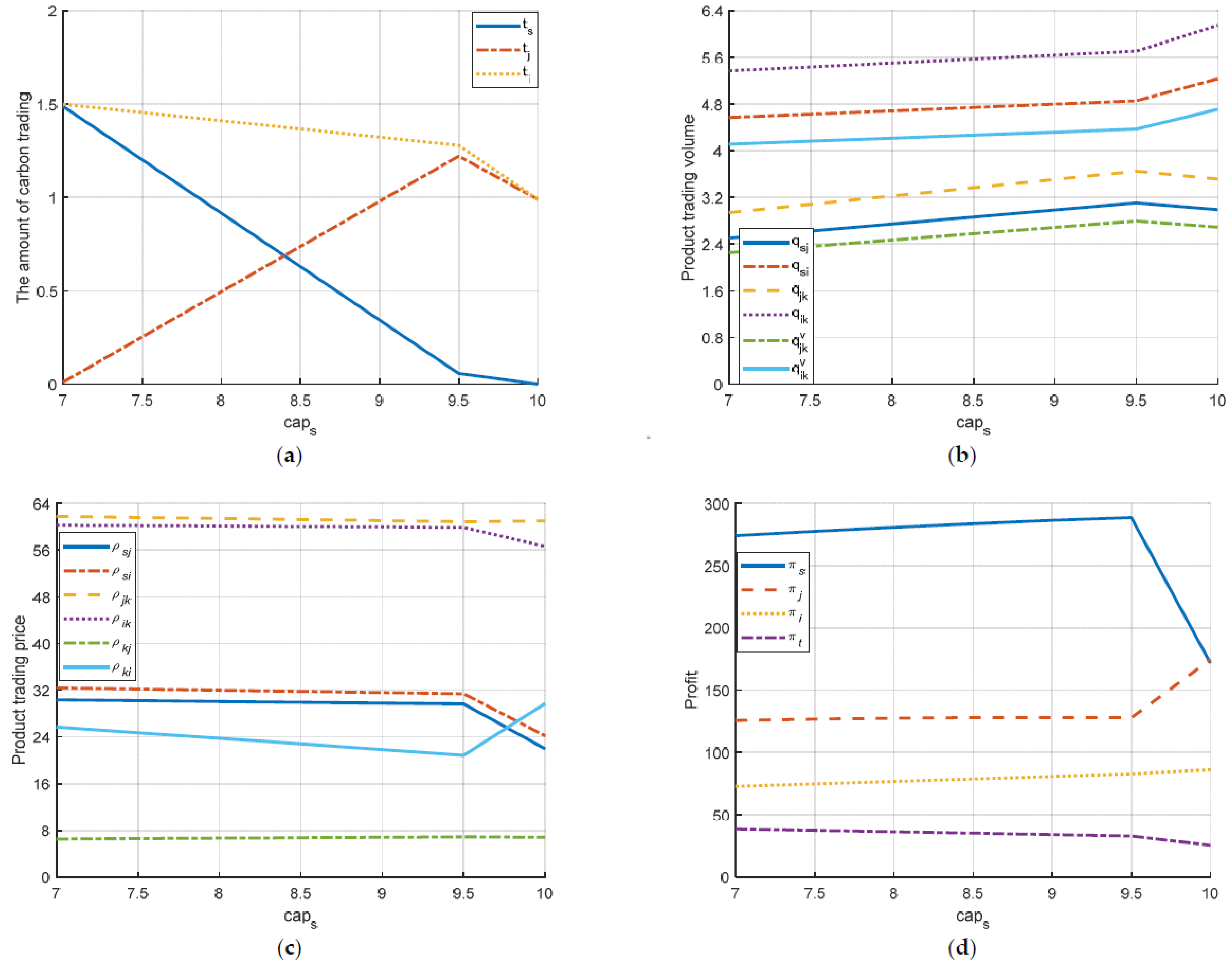
  • How does the carbon cap on high-emission enterprises affect the production and remanufacturing quantities, product transaction volumes, carbon trading volumes and members’ profits in a CLSCN?
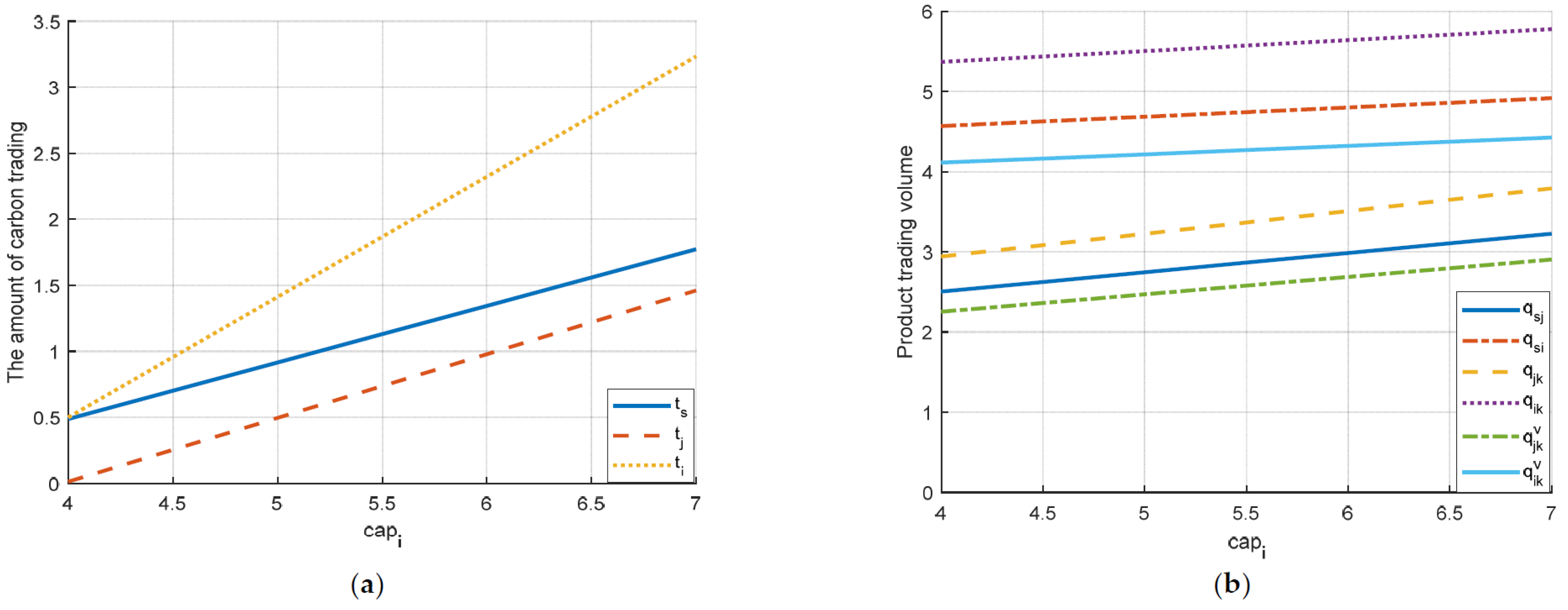
  • How does the carbon cap on low-emission enterprises affect the production and remanufacturing quantities, product transaction volumes, carbon trading volumes and members’ profits in a CLSCN?
  • How does the collection rate of EOL products affect the equilibrium and carbon trading strategies of a CLSCN?
Compared with the previous literature, this paper makes the following three contributions. (1) We introduce the carbon trading center as a platform for carbon trading between high-emission and low-emission enterprises and apply carbon trading volumes as decision variables for both types of enterprises. Moreover, in contrast to the existing literature, this study allows carbon trading both between the same types of decision-makers in the same tier in the horizontal direction and between upstream and downstream decision-makers in the vertical direction in the CLSCN. (2) In contrast to the use of Stackelberg game theory to study a simple linear CLSC in the existing literature, this paper utilizes variational inequality theory to establish a game model among different members of the CLSCN. (3) We find that the government should choose reasonable and moderate carbon caps for both high- and low-emission enterprises to balance the CLSCN members’ economic interests, carbon emissions, as well as resources utilization rate. Moreover, the government should not blindly pursue a high collection rate target.
The remainder of the paper is organized as follows. Section 2 reviews the related literature. Section 3 states the assumptions and notations used. Section 4 describes the optimal behaviors of different members of the CLSCN under CAT regulation and then obtains the equilibrium conditions of the whole CLSCN. Section 5 provides an algorithm for solving the model numerically, and then analyzes the results of numerical examples. Section 6 presents managerial insights. Section 7 summarizes the research results and suggests future research directions.

2. Literature Review

Aiming to study the impacts of CAT regulation on the operations of a multi-echelon CLSCN, our work is closely related to CLSCN equilibrium and the operational decisions of firms under CAT regulation. Therefore, the following section reviews the relevant literature in terms of these two aspects and clarifies differences between previous studies and ours.

2.1. Equilibrium Decisions in the Closed-Loop Supply Chain Network

A supply chain is a functional structure that integrates manufacturing and distribution. Its development has always been the interest of many scholars, and recently the research focus has gradually shifted from the forward supply chain [19,20] to a CLSC that involves the collection and remanufacturing of EOL products [21,22,23]. Furthermore, in order to gain a competitive advantage, many enterprises have multiple buyer–seller relationships with upstream and downstream firms, so the CLSC also gradually develops into a CLSCN with a hierarchical network structure [24,25]. With this in mind, several researchers have investigated the equilibrium decisions from a CLSCN perspective.
Yang et al. [26] formulated a variational inequality model for a CLSCN composed of five tiers represented by raw material suppliers, manufacturers, retailers, consumers and third-party recyclers. Qiang et al. [27] constructed a decentralized CLSCN model with manufacturer collection. He focused on the effects of competition, distribution channel investments, random yield and demand uncertainties on equilibriums. Qiang [28] developed a two-period CLSCN model taking account of product remanufactureability and the consumers’ different valuations between new and remanufactured products simultaneously. Hamdouch et al. [29] formulated a decentralized CLSCN model in which both demands and returns are random and price-sensitive. Chan et al. [30] examined a dynamic CLSCN equilibrium model based on evolutionary variational inequality theory. Wang et al. [31] studied the impacts of WEEE legislation on a CLSCN with retailer collection. Fu et al. [32] developed a coupled CLSCN model dealing with heterogeneous products facing different market demands.
Although the above literature establishes a good basis for this study by exploring the CLSCN equilibrium, regarding the impact of carbon emission regulations on the CLSCN is relatively scarce. Tao et al. [16] studied a CLSCN equilibrium problem in a multi-period planning horizon based on two types of mandatory carbon emission policies: global carbon emission policy and periodic carbon emission policy. However, they also did not address carbon trading within the same tier or between multiple tiers. Thus, this study aims to fill this gap by simultaneously modeling product transactions and carbon trading behaviors in a CLSCN under CAT regulation.

2.2. Impact of Cap-and-Trade Regulation on the Decision-Making of Firms

Another focus related to our research is the CAT regulation of supply chains, which is a highly relevant topic in areas such as inventory management, green supply chain and corporate operations research [33,34,35,36]. In terms of enterprise operational decisions, Chang et al. [37] studied the optimal production/remanufacturing decisions in a two-stage CLSC model with substitutable demands. Sarkar et al. [38] considered smart production systems with carbon emissions and revealed that reduced carbon and better products could be achieved. In the supply chain field, Xu and Bai [8] researched the coordination mechanism in a sustainable supply chain under CAT regulation. Ji and Yang [39] analyzed a forward supply chain model that incorporates both CAT policy and consumer preference for low-carbon products. Xu and Zhao [5] studied carbon emission reduction decisions in a dual-channel supply chain subjected to CAT regulation. Kushwaha and Rao [40] studied the channel selection of collection activity in a reverse supply chain. However, the above studies primarily focus on the equilibrium decisions of a forward supply chain or CLSC with a linear structure under CAT regulation, but do not include a CLSCN. The only exception is Allevi et al. [41], who considered a situation in which manufacturers in a CLSCN are bound by EU-ETS (a form of CAT regulation). However, this paper did not consider the case in which both carbon trading and product trading subnets co-exist in the CLSCN. Moreover, they also did not treat carbon trading volume as a decision variable of enterprises. Table 1 compares the differences between related works and this paper.
From the above discussions, the following research gaps are summarized: (1) Most of the previous studies on carbon trading, except for Allevi et al. [41], focused on simple/linear supply chains. (2) Few studies have involved carbon trading centers in CLSCs under carbon trading regulation. (3) Most previous studies have not treated the carbon trading volume as a decision variable. (4) Previous studies have mainly explored the situation in which carbon trading occurs between upstream and downstream decision-makers, while few of them have examined carbon trading in the horizontal direction among the same types of decision-makers in the same tier of the CLSCN.

3. Assumptions and Notations

We consider a three-echelon CLSCN consisting of S suppliers, J high-emission manufacturers, I low-emission manufacturers and K demand markets, in which all the manufacturers produce new products by raw materials, and are also responsible for collection and remanufacturing EOL products. Figure 1 is a simple diagram that represents a CLSC super-network model. There are two dotted areas: one is a product trading subnet with two types of manufacturers, who sell both new and remanufactured products to the demand market, and the other is a carbon trading subnet with a carbon trading center introduced as a platform, in which carbon credits are traded between high- and low-emission enterprises. In addition, Figure 1 includes three types of lines: the bold and solid lines from the carbon trading center to suppliers and manufacturers denote carbon trading; the solid lines from suppliers and manufacturers to demand markets indicate product trading; and the dotted lines show the collection of EOL products from demand markets by both types of manufacturers.
Manufacturers generate carbon emissions in the process of production and remanufacturing, and specific carbon emissions are measured according to the established method. We assume that carbon trading centers can balance the flow of carbon trading and control its volume. Moreover, the government assigns a certain carbon quota to enterprises that participate in carbon trading before production and remanufacturing. If each enterprise generates more carbon emissions than the allocated carbon cap during the production and remanufacturing cycle, it can buy the required carbon credits from the carbon trading center; conversely, it can sell its remaining carbon credits in the carbon trading center.
Considering the complexities of our research problem, we make the following assumptions, and define the corresponding model parameters, decision variables and function symbols in Table 2. Note that we use the superscript asterisk “ ” to label the equilibrium solutions in the paper.
Assumption 1. For both types of manufacturers, there is no difference between their new and remanufactured products, and the two kinds of products are sold at the same price in the consumer market [16].
Assumption 2. Both types of manufacturers produce homogeneous products, so there is a competitive or substitution relationship between products [17]. This assumption is consistent with the reality. For example, some Chinese domestic brands are becoming more and more homogeneous now (Huawei mobile phones and Xiaomi mobile phones are similar not only in appearance, but also in configuration), which leads to intensified competition between them.
Assumption 3. Compared with high-emission manufacturers, low-emission manufacturers have higher production costs with extra investments in green technology, more expensive environmental materials and lower remanufacturing costs [38]. In addition, for both types of manufacturers, their remanufacturing costs for EOL products are lower than production costs made from raw materials, which provides an economic basis for the remanufacturing industry to generate high added value [42].
Assumption 4. Remanufacturing is widely regarded as a low-carbon alternative to new manufacturing [37,40]. Thus, the carbon emission in the process of remanufacturing unit EOL products is lower than that of manufacturing unit new product by raw materials for both two types of manufacturers in our model.
Assumption 5. Without loss of generality, it is assumed that suppliers and high-emission manufacturers always emit more than the government’s assigned carbon cap, while low-emission manufacturers always emit less than the carbon cap. One can also consider the case that the suppliers are low-emission enterprises who emit less than the carbon cap.
Assumption 6. Consistent with previous CLSCN literature [16,29], all the related production/remanufacturing cost functions and transaction cost functions in the model are continuous and differentiable convex functions.

4. Model Formulation

Let us consider a three-echelon CLSCN, in which S suppliers sell raw materials to J high-emission manufacturers and I low-emission manufacturers. Both types of manufacturers produce new products by raw materials, and collect and remanufacture the EOL products generated by K demand markets. They sell both new and remanufactured products in the market.
In this section, we separately derive the optimal conditions for members in each tier of the CLSCN, and then provide the equilibrium conditions of the entire CLSCN.

4.1. The Optimal Behavior of Suppliers

First, we focus on the optimal behavior of supplier s who seeks to maximize its profit by selling raw materials to two types of manufacturers. Hence, considering the transactions between supplier s and high-emission manufacturer j and low-emission manufacturer i , supplier s makes decisions on q s , q s j , q s i and t s , which can be described as follows:
π s = max s = 1 S [ ρ s j q s j + ρ s i q s i c s j ( q s j ) c s i ( q s i ) f s ( q s ) ω t s ε t s ]
s . t α s q s c a p s t s = 0
i = 1 I q s i + j = 1 J q s j q s = 0
j , k , ρ s j 0 , ρ s i 0 , q s 0 , q s j 0 , q s i 0 , t s 0
The profit of supplier s in Equation (1) results from the difference between the raw materials sales revenue s = 1 S ρ s j q s j + ρ s i q s i and the sum of the transaction costs between the supplier and two types of manufacturers c s j ( q s j ) and c s i ( q s i ) , the production cost of the materials f s ( q s ) , the expense for buying carbon credits in the carbon trading center ω t s and the commission fees charged by the carbon trading center ε t s . Constraint (2) states the volume of carbon emissions generated by the supplier minus the government-mandated carbon cap is equal to the volume of carbon credits bought from the carbon trading center. Constraint (3) denotes the total quantities provided by supplier s are equal to the total purchasing quantities by both types of manufacturers from the supplier.
We assume that the Lagrange multipliers corresponding to Constraints (2) and (3) are λ s and θ s , respectively, and λ 1 = ( λ s ) S × 1 R S , θ = ( θ s ) S × 1 R S . Non-cooperative Nash games are played between different suppliers; therefore, combined with VI theory, the profit maximization goal of all suppliers can be described as: determine ( Q s , Q 1 1 , Q 1 2 , t 1 , λ 1 , θ ) Ω S , satisfying:
s = 1 S [ f s ( q s ) / q s + α s λ s θ ] × ( q s q s ) + s = 1 S i = 1 I [ c s i ( q s i ) / q s i ρ s i + θ ] × ( q s i q s i ) + s = 1 S j = 1 J [ c s j ( q s j ) / q s j ρ s j + θ ] × ( q s j q s j ) + s = 1 S ( ω + ε λ s ) × ( t s t s ) + s = 1 S ( c a p s α s q s + t s ) × ( λ s λ s ) + s = 1 S ( q s i = 1 I q s i j = 1 J q s j ) × ( θ θ ) 0
( Q s , Q 1 1 , Q 1 2 , t 1 , λ 1 , θ ) Ω S , where Ω S = { ( Q s , Q 1 1 , Q 1 2 , t 1 , λ 1 , θ ) R + S J + S I × R + S × R S } .
The first term in VI (4) shows that when q s > 0 , then λ s = 1 / α s [ θ f s ( q s ) / q s ] , which is the difference of Lagrange multipliers θ and the marginal supplying cost divided by α s ; for the fourth term in VI (4), we notice that when the carbon trading price ω plus the commission ε is exactly equal to λ s , supplier s will consider buying carbon credits from the carbon trading center; otherwise, the manufacturer will not purchase it. The second and third terms in VI (4) indicate that, as the marginal transaction cost between supplier s and manufacturer x increases, the equilibrium raw materials price ρ s x charged by the supplier also increases.

4.2. The Optimal Behavior of High-Emission Manufacturers

Each high-emission manufacturer j makes decisions on q j k , q j k v , q k j and t j to maximize its profit, which can be described as:
π j = max k = 1 K [ ρ j k q j k c j k ( q j k ) q k j ρ k j f j ( q J K v ) ε t j ω t j c j ( q k j ) f j ( β , q k j ) ] s = 1 S ( ρ s j q s j + c ^ s ( q s j ) )
s . t .     μ k = 1 K q j k k = 1 K q k j
s = 1 S η q s j = k = 1 K q j k v
k = 1 K q j k q j k v + β k = 1 K q k j
k = 1 K α j r q k j + k = 1 K α j q j k c a p j t j = 0
j , k , ρ j k 0 , ρ k j 0 , q j k 0 , q j k v 0 , q k j 0 , q s j 0 , t j 0
The high-emission manufacturer j generates revenue from the sale of the new and remanufactured products ρ j k q j k , while incurs the transaction costs with the consumer market c j k ( q j k ) , the production cost of new products f j ( q J K v ) , the costs of buying back EOL products q k j ρ k j from the consumers, the disposal cost c j ( q k j ) and remanufacturing cost f j ( β , q k j ) for the EOL products, the costs of dealing with suppliers for raw materials s = 1 S ( ρ s j q s j + c ^ s ( q s j ) ) , the expense for buying carbon credits in the carbon trading center ω t j and the commission fees charged by the carbon trading center ε t j . Then the profit of manufacturer j in Equation (5) is the difference between the revenue and costs listed above. Constraint (6) shows that the total collection quantity of EOL products by high-emission manufacturer j from all demand markets should not be lower than the minimum amount that the government requires it to collect. Constraint (7) denotes flow conservation, which ensures that the quantity of new products produced by high-emission manufacturer j is equivalent to the conversion quantity of raw materials. Constraint (8) indicates that the total quantity of products sold by manufacturer j to all the demand markets should not be larger than the sum of the quantity of products made from raw materials and remanufactured from EOL products. Constraint (9) denotes that the high-emission manufacturer will only purchase carbon credits from the carbon trading center if its carbon emissions are higher than the government’s carbon caps.
Let ζ 1 j , ζ 2 j , ζ 3 j and λ j be the Lagrange multipliers regarding Constraints (6)~(9), respectively, and ζ 1 1 = ( ζ 1 j ) J × 1 R + J , ζ 1 2 = ( ζ 2 j ) J × 1 R + J , ζ 1 3 = ( ζ 3 j ) J × 1 R + J , λ 2 = ( λ j ) J × 1 R J . The non-cooperative Nash games are played between different high-emission manufacturers, and combined with the VI theory, the profit maximization goal of all high-emission manufacturers therefore can be described as: determine ( Q 2 1 , q 2 v , Q 2 2 , Q 1 1 , t 2 , ζ 1 1 , ζ 1 2 , ζ 1 3 , λ 2 ) Ω J , satisfying:
j = 1 J k = 1 K [ ( c j k ( q j k ) ) / q j k + λ j α j + μ ζ 1 j + ζ 2 j ρ j k ] × ( q j k q j k ) + j = 1 J k = 1 K [ ( f j ( q J K v ) ) / q j k v ζ 2 j + ζ 3 j ] × ( q j k v q j k v ) + j = 1 J k = 1 K [ ( c j ( q k j ) + f j ( β , q k j ) ) / q k j + ρ k j + λ j α j r ζ 1 j β ζ 2 j ] × ( q k j q k j ) + j = 1 J s = 1 S [ ( c s ( q s j ) / q s j ) + ρ s j η ζ 3 j ] × ( q s j q s j ) + j = 1 J ( ω + ε λ j ) × ( t j t j ) + j = 1 J ( c a p j k = 1 K α j r q k j k = 1 K α j q j k + t j ) × ( λ j λ j ) + j = 1 J ( k = 1 K q k j μ k = 1 K q j k ) × ( ζ 1 j ζ 1 j ) + j = 1 J ( k = 1 K q j k v + β k = 1 K q k j k = 1 K q j k ) × ( ζ 2 j ζ 2 j ) + j = 1 J ( s = 1 S η q s j k = 1 K q j k v ) × ( ζ 3 j ζ 3 j ) 0
( Q 2 1 , q 2 v , Q 2 2 , Q 1 1 , t 2 , ζ 1 1 , ζ 1 2 , ζ 1 3 , λ 2 ) Ω J
where Ω J = { ( Q 2 1 , q 2 v , Q 2 2 , Q 1 1 , t 2 , ζ 1 1 , ζ 1 2 , ζ 1 3 , λ 2 ) R + S J + 3 J K × R + 4 J × R J } .
According to the second term of VI (10), when q j k v > 0 , ζ 2 j = ( f j ( q J K v ) ) / q j k v + ζ 3 j ; the first term in VI (10) shows that when q j k > 0 , ρ j k = ( c j k ( q j k ) ) / q j k + λ j α j μ ζ 1 j + ζ 2 j , that is, the equilibrium transaction price ρ j k is related to the marginal transaction cost, the per-unit carbon emission quantity during production, the collection rate and the Lagrange multipliers of the associated constraints; from the third term, when the sum of high-emission manufacturer j ’s marginal disposal cost and remanufacturing cost of EOL product decreases, the EOL product transaction price ρ k j charged by the manufacturer increases. Thus, in order to promote collection and remanufacturing activities, the high-emission manufacturers will be willing to collect EOL products at a higher price when the disposal and remanufacturing costs of EOL products such as test, classification and remanufacturing are reduced.

4.3. The Optimization Behavior for Low-Emission Manufacturers

Each low-emission manufacturer i makes decisions on q i k , q i k v , q k i and t i to maximize its profit, which can be described as:
π i = max k = 1 K [ ρ i k q i k c i k ( q i k ) q k i ρ k i f i ( q I K v ) ε t i + ω t i c i ( q k i ) f i ( β , q k i ) ] s = 1 S ( ρ s i q s i + c ^ s ( q s i ) )
s . t . μ k = 1 K q i k k = 1 K q k i
s = 1 S η q s i = k = 1 K q i k v
k = 1 K q i k q i k v + β k = 1 K q k i
c a p i k = 1 K α i r q k i k = 1 K α i q i k = t i
i , k , ρ i k 0 , ρ k i 0 , q i k 0 , q i k v 0 , q k i 0 , q s i 0 , t i 0
The revenue of the low-emission manufacturer i comprises revenue from the sale of new and remanufactured products ρ i k q i k and carbon emission volume sales revenue ω t i , while the costs comprise the transaction costs with the consumer markets c i k ( q i k ) , the production cost of new products f i ( q I K v ) , the costs of buying back EOL products q k i ρ k i , the disposal cost c i ( q k i ) and remanufacturing cost f i ( β , q k i ) for the EOL products, the costs of dealing with suppliers for raw materials s = 1 S ( ρ s i q s i + c ^ s ( q s i ) ) and the commission fees charged by the carbon trading center ε t i . Then the profit of manufacturer i in Equation (11) results from the difference between revenues and costs listed above. Constraint (12) shows that the total collection quantity of EOL products by low-emission manufacturer i should not be lower than the minimum amount that the government requires it to collect. Constraint (13) denotes flow conservation, which ensures that the quantity of the supplier s ’s converted raw materials is equal to the quantity of new products produced. Constraint (14) indicates that the total amount of products sold by low-emission manufacturer i to the demand markets should not be larger than the sum of the new products made from raw materials and the remanufactured products made from EOL products. Constraint (15) indicates that the low-emission manufacturers trade the surplus carbon emissions that fall below the government-mandated carbon caps in the carbon trading center.
Non-cooperative Nash games are played between different low-emission manufacturers, and combined with the VI theory, therefore, the profit maximization goal of all low-emission manufacturers can be described as: determine ( Q 3 1 , q 3 v , Q 3 2 , Q 1 2 , t 3 , ζ 2 1 , ζ 2 2 , ζ 2 3 , λ 3 ) Ω I , satisfying:
i = 1 I k = 1 K [ ( c i k ( q i k ) ) / q i k + λ i α i + μ ζ 1 i + ζ 2 i ρ i k ] × ( q i k q i k ) + i = 1 I k = 1 K [ ( f i ( q I K v ) ) / q i k v ζ 2 i + ζ 3 i ] × ( q i k v q i k v ) + i = 1 I k = 1 K [ ( c i ( q k i ) + f i ( β , q k i ) ) / q k i + ρ k i + λ i α i r ζ 1 i β ζ 2 i ] × ( q k i q k i ) + i = 1 I s = 1 S [ ( c ^ s ( q s i ) / q s i ) + ρ s i η ζ 3 i ] × ( q s i q s i ) + i = 1 I ( λ i + ε ω ) × ( t i t i ) + i = 1 I ( c a p i k = 1 K α i r q k i k = 1 K α i q i k t i ) × ( λ i λ i ) + i = 1 I ( k = 1 K q k i μ k = 1 K q i k ) × ( ζ 1 i ζ 1 i ) + i = 1 I ( k = 1 K q i k v + β k = 1 K q k i k = 1 K q i k ) × ( ζ 2 i ζ 2 i ) + i = 1 I ( s = 1 S η q s i k = 1 K q i k v ) × ( ζ 3 i ζ 3 i ) 0
( Q 3 1 , q 3 v , Q 3 2 , Q 1 2 , t 3 , ζ 2 1 , ζ 2 2 , ζ 2 3 , λ 3 ) Ω I
where Ω I = { ( Q 3 1 , q 3 v , Q 3 2 , Q 1 2 , t 3 , ζ 2 1 , ζ 2 2 , ζ 2 3 , λ 3 ) R + S I + 3 I K × R + 4 I × R I } .
We set ζ 1 i , ζ 2 i , ζ 3 i and λ i as the Lagrange multipliers in Constraints (12)~(15), respectively. Let ζ 2 1 = ( ζ 1 i ) I × 1 R + I , ζ 2 2 = ( ζ 2 i ) I × 1 R + I , ζ 2 3 = ( ζ 3 i ) I × 1 R + I and λ 3 = ( λ i ) I × 1 R I . In addition, the analysis of equilibrium conditions for low-emission manufacturers is similar to those for high-emission manufacturers, and is not given here in detail.

4.4. The Optimal Condition of Demand Markets

In the process of products sales, for the products of high-emission manufacturers, the transaction occurs only when the price p k j paid by customers is equivalent to the sum of the transaction price ρ j k and the transaction cost c ^ j k ( q j k ) in demand markets. Using the notation defined above, the complementary relationship related to products sales/purchase between manufacturers and demand markets can be expressed as:
ρ j k + c ^ j k ( q j k ) { p k j , q j k = 0 = p k j , q j k > 0
Similar to the relationship between high-emission manufacturers and demand markets, there is also a complementary relationship related to products sales/purchase between low-emission manufacturers and demand markets that can be described as:
ρ i k + c ^ i k ( q i k ) { p k i , q i k = 0 = p k i , q i k > 0
In addition, according to Tao et al. [16] and Hamdouch et al. [29], for high-emission manufacturers, the complementary relationship between the price p k j paid by consumers in demand markets and the demand quantity can be expressed as:
{ d k j ( p k j ) = j = 1 J q j k , p k j 0 d k j ( p k j ) j = 1 J q j k , p k j = 0
For low-emission manufacturers, the demand function can be similarly expressed as:
{ d k i ( p k i ) = i = 1 I q i k , p k i 0 d k i ( p k i ) i = 1 I q i k , p k i = 0
In the process of EOL products collection, we notice that the higher the transaction price of EOL products paid by manufacturers, the more willing consumers are to return EOL products to them. According to Tao et al. [16], for high-emission manufacturer j , the complementary relationship satisfied by the collection of EOL products can be expressed as:
c k ( q k j ) { = ρ k j , q k j > 0 ρ k j , q k j = 0
s . t . k = 1 K q k j k = 1 K q j k
Constraint (21) describes the condition that transaction occurs between the demand market k and the manufacturer j for the EOL products. Constraint (22) ensures that for each high-emission manufacturer j , the quantity of EOL products that it collects from the demand markets should not exceed its total sales volume in demand markets. Similarly, for each low-emission manufacturer i , the complementary relationship satisfied by the collection of EOL products can be expressed as:
c k ( q k i ) { = ρ k i , q k i > 0 ρ k i , q k i = 0
s . t . k = 1 K q k i k = 1 K q i k
Constraints (17)~(24) are required for the equilibrium of the demand market, which can be described by the VI in VI (25): determining ( Q 2 1 , Q 2 2 , Q 3 1 , Q 3 2 , P 1 , P 2 , λ 4 1 , λ 4 2 ) Ω K , satisfying:
k = 1 K i = 1 I [ c k ( q k i ) ρ k i + λ k i ] × ( q k i q k i ) + i = 1 I k = 1 K [ ρ i k + c ^ i k ( q i k ) p k i λ k i ] × ( q i k q i k ) + k = 1 K [ i = 1 I q i k d k i ( p k i ) ] × ( p k i p k i ) + i = 1 I ( k = 1 K q i k k = 1 K q k i ) × ( λ k i λ k i ) + k = 1 K j = 1 J [ c k ( q k j ) ρ k j + λ k j ] × ( q k j q k j ) + j = 1 J k = 1 K [ ρ j k + c ^ j k ( q j k ) p k j λ k j ] × ( q j k q j k ) + k = 1 K [ j = 1 J q j k d k j ( p k j ) ] × ( p k j p k j ) + j = 1 J ( k = 1 K q j k k = 1 K q k j ) × ( λ k j λ k j ) 0
( Q 2 1 , Q 2 2 , Q 3 1 , Q 3 2 , P 1 , P 2 , λ 4 1 , λ 4 2 ) Ω K
where Ω K = { ( Q 2 1 , Q 2 2 , Q 3 1 , Q 3 2 , P 1 , P 2 , λ 4 1 , λ 4 2 ) R + 3 I K + 3 J K × R + I + J } .
The corresponding Lagrange multipliers of Constraints (22) and (24) are λ k j and   λ k i , respectively, and let   λ 4 1 = ( λ k j ) k × 1 R + K ,   λ 4 2 = ( λ k i ) k × 1 R + K . From the first and fifth term of VI (25), we note that when q k x > 0 , ρ k x = c k ( q k x ) + λ k x , that is, the optimal transaction price of EOL products ρ k x paid by the manufacturer is equal to the sum of the disutility function and the Lagrange multiplier λ k x .

4.5. The Optimal Behavior of Carbon Trading Centers

According to the assumptions, in the carbon trading subnet, the supply of carbon emissions comes from low-emission enterprises and the demand for carbon emissions comes from high-emission enterprises. Among them, low-emission enterprises only include low-emission manufacturers, while high-emission enterprises include suppliers and high-emission manufacturers. Furthermore, the carbon trading center charges transaction fees on both sides according for a fixed proportion of the trading volume.
We note that the carbon emission demand of suppliers is s = 1 S t s = s = 1 S ( α s q s c a p s ) , the carbon emission demand of high-emission manufacturers is j = 1 J t j = j = 1 J ( k = 1 K α j q j k + k = 1 K α j r q k j c a p j ) , and the carbon emission supply of low-emission manufacturers is i = 1 I t i = i = 1 I ( c a p i k = 1 K α i q i k k = 1 K α i r q k i ) . Hence, the profit maximization goal of carbon trading center t can be described as:
π t = max [ s = 1 S ( ε t s c s t ( t s ) ) + j = 1 J ( ε t j c j t ( t j ) ) + i = 1 I ( ε t i c i t ( t i ) ) ]
s . t s = 1 S t s + j = 1 J t j i = 1 I t i
q s j 0 , q s i 0 , q j k 0 , q i k 0
The profit of carbon trading centers in Equation (26) comprises two parts: commission fees from both types of manufacturers and suppliers s = 1 S ε t s + ε t i + ε t j and the transaction cost borne by the carbon trading center s = 1 S c s t ( t s ) + c i t ( t i ) + c j t ( t j ) . Constraint (27) indicates that the carbon emissions purchased by high-emission enterprises are not larger than those sold by low-emission enterprises.
We set the Lagrange multiplier of Constraint (27) as λ c , and let   λ 5 = ( λ c ) 1 × 1 R . Based on the fact that the equilibrium decision points for suppliers and producers in the carbon trading are q s j 0 , q s i 0 and q j k 0 , q i k 0 , and these should also be the equilibrium solutions to the following VI: determining ( t 2 , t 1 , λ 4 ) Ω T , satisfying:
s = 1 S [ c s t ( t s ) / t s ε + λ c ] × ( t s t s ) + j = 1 J [ c j t ( t j ) / t j ε + λ c ] × ( t j t j ) + i = 1 I [ c i t ( t i ) / t i ε λ c ] × ( t i t i ) + ( i = 1 I t i j = 1 J t j s = 1 S t s ) × ( λ c λ c ) 0
( t 1 , t 2 , t 3 , λ 5 ) Ω T
where Ω T = ( t 1 , t 2 , t 3 , λ 5 ) R + S + J + I + R .

4.6. The Optimal Behavior of Closed-Loop Supply Chain Networks

Finally, the entire CLSCN and carbon trading network can reach Nash equilibrium only when the product transaction quantities, carbon trading volumes and product trading prices between members at all tiers in the CLSCN meet the sum of the above five VIs. Then the VI for the entire CLSCN can be expressed as: determine ( q 1 v , q 2 v , Q s , Q 1 1 , Q 1 2 , Q 2 1 , Q 2 2 , t 1 , t 2 , λ 1 , θ , λ 2 , ζ 1 1 , ζ 1 2 , ζ 2 1 , ζ 2 2 , P 1 , P 2 , λ 3 1 , λ 3 2 , λ 4 ) Ω , satisfying:
s = 1 S [ f s ( q s ) q s + α s λ s θ ] × ( q s q s ) + s = 1 S j = 1 J [ ( c s j ( q s j ) + c ^ s ( q s j ) ) q s j + θ η ζ 3 j ] × ( q s j q s j ) + s = 1 S i = 1 I [ ( c s i ( q s i ) + c ^ s ( q s i ) ) q s i + θ η ζ 3 i ] × ( q s i q s i ) + j = 1 J k = 1 K [ ( c j k ( q j k ) ) q j k + λ j α j + μ ζ 1 j + ζ 2 j + c ^ j k ( q j k ) p k j λ k j ] × ( q j k q j k ) + i = 1 I k = 1 K [ ( c i k ( q i k ) ) q i k + λ i α i + μ ζ 1 i + ζ 2 i + c ^ i k ( q i k ) p k i λ k i ] × ( q i k q i k ) + j = 1 J k = 1 K [ ( f j ( q J K v ) ) q j k v ζ 2 j + ζ 3 j ] × ( q j k v q j k v ) + i = 1 I k = 1 K [ ( f i ( q I K v ) ) q i k v ζ 2 i + ζ 3 i ] × ( q i k v q i k v ) + k = 1 K j = 1 J [ ( c j ( q k j ) + f j ( β , q k j ) ) q k j + c k ( q k j ) + λ k j + λ j α j r ζ 1 j β ζ 2 j ] × ( q k j q k j ) + k = 1 K i = 1 I [ ( c i ( q k i ) + f i ( β , q k i ) ) q k i + c k ( q k i ) + λ k i + λ i α i r ζ 1 i β ζ 2 i ] × ( q k i q k i ) + s = 1 S [ c s t ( t s ) t s λ s + λ c + ω ] × ( t s t s ) + j = 1 J [ c j t ( t j ) t j λ j + λ c + ω ] × ( t j t j ) + i = 1 I [ c i t ( t i ) t i + λ i λ c ω ] × ( t i t i ) + s = 1 S ( c a p s i = 1 I α s q s i j = 1 J α s q s j + t s ) × ( λ s λ s ) + s = 1 S ( q s i = 1 I q s i j = 1 J q s j ) × ( θ θ ) + j = 1 J ( c a p j k = 1 K α j r q k j k = 1 K α j q j k + t j ) × ( λ j λ j ) + i = 1 I ( c a p i k = 1 K α i r q k i k = 1 K α i q i k t i ) × ( λ i λ i ) + j = 1 J ( k = 1 K q j k k = 1 K q k j ) × ( λ k j λ k j ) + i = 1 I ( k = 1 K q i k k = 1 K q k i ) × ( λ k i λ k i ) + ( i = 1 I t i j = 1 J t j s = 1 S t s ) × ( λ c λ c ) + j = 1 J ( k = 1 K q k j μ k = 1 K q j k ) × ( ζ 1 j ζ 1 j ) + i = 1 I ( k = 1 K q k i μ k = 1 K q i k ) × ( ζ 1 i ζ 1 i ) + j = 1 J ( k = 1 K q j k v + β k = 1 K q k j k = 1 K q j k ) × ( ζ 2 j ζ 2 j ) + i = 1 I ( k = 1 K q i k v + β k = 1 K q k i k = 1 K q i k ) × ( ζ 2 i ζ 2 i ) + j = 1 J ( s = 1 S η q s j k = 1 K q j k v ) × ( ζ 3 j ζ 3 j ) + i = 1 I ( s = 1 S η q s i k = 1 K q i k v ) × ( ζ 3 i ζ 3 i ) + k = 1 K [ j = 1 J q j k d k j ( p k j ) ] × ( p k j p k j ) + k = 1 K [ i = 1 I q i k d k i ( p k i ) ] × ( p k i p k i ) 0
( q 1 v , q 2 v , Q s , Q 1 1 , Q 1 2 , Q 2 1 , Q 2 2 , t 1 , t 2 , t 3 , λ 1 , θ , λ 2 , λ 3 , ζ 1 1 , ζ 1 2 , ζ 1 3 , ζ 2 1 , ζ 2 2 , ζ 2 3 , P 1 , P 2 , λ 4 1 , λ 4 2 , λ 5 ) Ω
where Ω = Ω S × Ω J × Ω I × Ω K × Ω T .
Note that in VI (29), the transaction prices between different tiers, i.e., the endogenous variables defined above, are cancelled out. In order to get these transaction prices back, we need to obtain each transaction price through VIs (4), (10), (16) and (25). According to inequality (4), we obtain ρ s i = c s i ( q s i ) / q s i + θ and ρ s j = c s j ( q s j ) / q s j + θ ; according to inequality (10), we obtain ρ j k = ( c j k ( q j k ) ) / q j k + λ j α j μ ζ 1 j + ζ 2 j ; according to inequality (16), we obtain ρ i k = ( c i k ( q i k ) ) / q i k + λ i α i μ ζ 1 i + ζ 2 i ; according to inequality (25), we obtain ρ k i = c k ( q k i ) + λ k i and ρ k j = c k ( q k j ) + λ k j . The proof of the existence and uniqueness of solutions to VI (29) can refer to the related reference, e.g., Tao et al. [16], Yang et al. [26].

5. Numerical Examples

In this section, we conduct several numerical examples to obtain conclusions and discuss managerial insights. The relevant parameters are assumed as ε = 6.5 , ω = 1 , β = 0.9 , η = 0.9 , α s = 0.6 , α i = 0.3 , α j = 0.8 , α i r = 0.1 , α j r = 0.2 . Moreover, the cost and transaction functions involved in the examples are set as follows.
In the supplier tier, the cost function of producing raw materials ordered by both types of manufacturers is:
f s ( q s ) = 0.5 q s 2 + q s
In the manufacturer tier, the cost functions of raw materials purchased by both types of manufacturers are, respectively:
f j ( q J K v ) = ( k = 1 2 q j k v ) 2 + k = 1 2 q 1 k v × k = 1 2 q 2 k v + 1.2 k = 1 2 q j k v
f i ( q I K v ) = ( k = 1 2 q i k v ) 2 + k = 1 2 q 1 k v × k = 1 2 q 2 k v + 2 k = 1 2 q i k v
In the manufacturer tier, the remanufacturing cost functions of both types of manufacturers are, respectively:
f j ( β , q k j ) = 0.1 ( β q k j ) 2 + 0.8 β q k j
f i ( β , q k i ) = 0.1 ( β q k i ) 2 + 0.5 β q k i
In the supplier tier, the transaction cost function borne by suppliers in the transaction process with both types of manufacturers is:
c s x ( q s x ) = 0.5 q s x 2 + 1.5 q s x
Conversely, the cost function borne by both types of manufacturers in the transaction process with the suppliers is:
c ^ s ( q s x ) = 0.5 q s x 2 + 0.3 q s x
In the manufacturer tier, the trading cost function borne by both types of manufacturers in the process of selling products in the demand market is:
c x k ( q x k ) = 0.5 q x k 2 + 1.2 q x k
Conversely, the cost function borne by consumers in the process of purchasing products is:
c ^ x k ( q x k ) = 0.1 q x k 2 + 1
The disposal cost functions borne by both types of manufacturers in the process of disposing collected EOL products are, respectively:
c j ( q k j ) = q k j 2 + 2
c i ( q k i ) = q k i 2 + 1
In the carbon trading center tier, the cost functions borne by the carbon trading center in the carbon trading process with suppliers and both types of manufacturers are, respectively:
c s t ( t s ) = 0.01 t s 2
c i t ( t i ) = 0.03 t i 2
c j t ( t j ) = 0.05 t j 2
The disutility function that describes consumers selling EOL products to both types of manufacturers in the demand market is:
c k ( q k x ) = 0.5 k = 1 2 x = 1 2 q k x + 5
The demand functions of the demand market for products of low-emission and high-emission manufacturers are, respectively, as follows. (In contrast to Tao et al. [16], in our model, the market demand is divided into products of high-emission and low-emission manufacturers; furthermore, according to the assumption that there is a competitive or substitution relationship between the products produced by the two types of manufacturers, the product demand of one type manufacturer generally depends not only on the prices of this type manufacturers’ products, but also on the prices of the other type manufacturers’ products in the market.)
d k i ( p k i , p k j ) = 2 p k i p 3 k i + 0.3 p k j + 0.1 p 3 k j + 200
d k j ( p k i , p k j ) = 2.5 p k j p 3 k j + 0.3 p k i + 0.1 p 3 k i + 200
The main algorithms for solving the VI include the modified project algorithm and the logarithmic–quadratic proximal prediction–correction algorithm [16]. Because the modified project algorithm is simple in design and can simultaneously determine the equilibrium solutions and Lagrange multipliers, this paper uses this algorithm to solve the model, and the algorithm was programmed with MATLAB. We set the iteration step as 0.01, and the termination condition is that the error of two iterations is less than or equal to 10 8 . For more details on this algorithm, we refer readers to the procedure given by Tao et al. [16] and Hamdouch et al. [29]. In the following, we study the impact of changes in government-mandated carbon caps and the collection rate on the production quantities, transaction prices, carbon trading volumes, and profits of various enterprises in the three-echelon CLSCN, which has important management significance, and certain reference value for governments and enterprises.

5.1. Numerical Example 1

First, we examine the effects of government-mandated carbon caps on equilibrium solutions in detail. In particular, we fix the carbon caps on suppliers and change the carbon caps on two types of manufacturers in this example. Specifically, we let μ = 0.26 , c a p s = 8 , and let c a p j = 4 : 0.5 : 7 , c a p i = 4 : 0.5 : 7 . The variations in carbon emission quantities, product trading volumes and profits are shown in Table 3.
As shown in Table 3, as the carbon caps on both types of manufacturers increase with the same step size, all the manufacturers have more space to increase production quantities of new products and remanufacturing quantities of EOL products free of charge. It leads to the fact that the carbon credits high-emission manufacturers need to buy decrease. In contrast, since the carbon cap of suppliers remains the same, they have to buy more extra carbon credits from low-emission manufacturers due to more order quantities of raw materials from both types of manufacturers. Accordingly, the low-emission manufacturers can sell more carbon credits in the carbon trading center. The profits of both types of manufacturers continually improve with the increase of c a p i and c a p j , while the profits of suppliers first increase then decrease. The reason is that the changes of suppliers’ profits depend both on raw materials sales revenue and expenses for buying extra carbon credits. When c a p i and c a p j are relatively lower, the increased raw materials sales revenue outweighs the increased expenses for buying more carbon credits with the increase of carbon emission caps, then the profits of suppliers increase. On the contrary, if c a p i and c a p j exceed the thresholds (in this example they are 4.5), the increased raw materials sales revenue cannot compensate for the increased expenses for buying more carbon credits, the profits of suppliers decline.

5.2. Numerical Example 2

In this example, we fix the carbon caps on both types of manufacturers and change the carbon caps on suppliers. Specifically, we let μ = 0.26 , c a p j = 5 , c a p i = 5 , and c a p s = 7 : 0.5 : 10 . We observe variations in carbon emission quantities, product trading volumes and profits, and the details are shown in Figure 2.
In Figure 2a, we find that when the suppliers’ carbon cap increases, the carbon trading volumes of both suppliers and low-emission manufacturers have a decreasing trend, while the carbon trading volumes of high-emission manufacturers first increase rapidly and then decrease. The turning point appears at c a p s = 9.5 . From Figure 2b, it can be seen that the product trading volumes of high-emission manufacturers increase substantially when c a p s 9.5 but decrease after c a p s > 9.5 , while the product trading volume of low-emission manufacturers increase slowly when c a p s 9.5 and then increase rapidly after c a p s > 9.5 . Combined with Figure 2a,b, we can infer that when the carbon cap on suppliers exceeds 9.5, if the suppliers still increase the supply of raw materials to both types of manufacturers for their new products’ production, high-emission manufacturers will have to buy more carbon credits in the carbon trade center, but low-emission manufacturers have insufficient surplus carbon credits to sell. Thus, the suppliers will be forced to transact more with the low-emission manufacturers but less with high-emission manufacturers. As shown in Figure 2c, excessive product transactions between the suppliers and low-emission manufacturers lead to a sharp drop in the prices of raw materials for both types of manufacturers and selling prices of low-emission manufacturers. As a result, to recoup the loss resulted from lower margin sales benefit, the low-emission manufacturers turn to raising the buy-back price for EOL products dramatically after c a p s > 9.5 , and then acquire more EOL products to remanufacture. This measure contributes to the overall product supply for them, which is so call “bulk-cheap policy”. In addition, it can also be observed from Figure 2c that the product selling price and buy-back price for EOL products of high-emission manufacturers remain almost the same as the suppliers’ carbon cap increases.
Based on the analysis of carbon trading volumes, product trading volumes and prices from Figure 2a to Figure 2c, we can easily understand the changes of profits with c a p s in Figure 2d. That is, when c a p s 9.5 , the suppliers’ profits increase steadily in c a p s , and both two types of manufacturers are also better off by a small margin. When c a p s > 9.5 , the suppliers’ profits suffer a cliff-like drop due to the decrease of raw material price, while the high-emission manufacturers benefit a lot from it. For low-emission manufacturers, “bulk-cheap policy” can compensate for the decrease of lower selling price, so their profits still keep increasing. The profit of carbon trading center decreases all the time due to the decrease of carbon trading volumes with c a p s increasing from 7 to 10.
This example implies that if the government restricts the suppliers’ carbon cap in a reasonable range, it can not only create a “win-win-win” situation for suppliers, high-emission manufacturers and low-emission manufacturers, but also reduce the carbon credits purchased by the suppliers and high-emission manufacturers in the carbon trading center.

5.3. Numerical Example 3

The above two sections analyze the impacts of changes in carbon caps at different tiers in the CLSCN. Subsequently, we will investigate the influences of carbon caps on two kinds of enterprises (high-emission enterprises and low-emission enterprises) on equilibrium solutions. As given in the above assumptions, suppliers and high-emission manufacturers are classified as high-emission enterprises, while low-emission manufacturers belong to low-emission enterprises.
In this section, we fix the carbon caps on high-emission enterprises and change those on low-emission enterprises. Specifically, we let μ = 0.26 , c a p s = 8 , c a p j = 5 and c a p i = 4 : 0.5 : 7 . Then we observe variations in the carbon emission quantities, product trading volumes and profits, and the details are shown in Figure 3.
Figure 3a,b show that, with the increase of carbon cap on low-emission enterprises (low-emission manufacturers), all the enterprises’ carbon trading volumes and product trading volumes between two types of enterprises increase. That is, a higher carbon cap on low-emission enterprises represents that they have more residual carbon credits to sell to the high-emission enterprises (suppliers and manufacturers) in the carbon emission center, and then boost the economic activities of the suppliers and manufacturers. It is also interesting to find from Figure 3b that the product trading volumes related to low-emission manufacturers are less sensitive to changes in their carbon cap than those of high-emission manufacturers, implying that the low-emission manufacturers are in a dominant position in the product transaction process.
From Figure 3c, it can be seen that the increase in the provision of raw materials from suppliers leads to a decrease of selling price of raw materials. Therefore, the low-emission manufacturers prefer to make use of more raw materials to produce new products rather than produce remanufactured products by EOL products. Accordingly, they reduce the buy-back price to decrease the collection quantities of EOL products. From Figure 3d, we can find that as c a p i increases, the suppliers suffer losses since the profit increment resulted from the increase in raw materials supply is lower than the profit reduction due to both the decrease in raw materials selling prices and the increase of expenses for purchasing carbon credits. In contrast, an opposite changing trend arises for the profits of manufacturers and carbon trading center, mainly owing to the increase of product transaction volumes and carbon trading volumes with c a p i .

5.4. Numerical Example 4

In this section, we assume that the carbon cap on low-emission manufacturers is fixed and change the carbon cap on high-emission enterprises (suppliers and high-emission manufacturers); specifically, we let μ = 0.26 , c a p i = 5 , c a p s = 7 : 0.5 : 10 and c a p j = 4 : 0.5 : 7 . The variations in the carbon trading quantities, product trading volumes and profits are listed in Table 4.
Table 4 shows that increasing the carbon caps on high-emission enterprises will increase (decrease) the product (carbon) trading volumes of each enterprise. In other words, when the carbon quotas allocated by the government are relatively abundant for high-emission enterprises, they will purchase fewer carbon credits from the carbon trading center. Consequently, the carbon trading center is less profitable, and this will also cause a greater burden to the environment. In addition, with the increase of the carbon caps for suppliers and high-emission manufacturers at the same pace, the profits of both types of manufacturers show an upward trend with respect to products sales volumes, while that of suppliers first increase and then decrease. Specifically, the profit of suppliers reaches the maximum at the point ( c a p s , c a p j ) = ( 9 , 6 ) . This changing trend of suppliers’ profit still depends on the joint influences of transaction quantities and selling prices of raw materials, and the expenses for purchasing carbon credits, which can be explained in a similar way as Numerical example 3.
Hence, based on the above analysis, the setting of carbon caps by government on high-emission enterprises should balance the CLSCN members’ economic interests and carbon emissions. In this example, the carbon caps ( c a p s , c a p j ) = ( 9 , 6 ) for high-emission enterprises can realize profit maximization of suppliers, and make both types of manufacturers at a relatively higher level, as well as generate not too high carbon emissions.

5.5. Numerical Example 5

In this section, we explore the impacts of minimum collection rate of EOL products μ set by government on equilibrium solutions in detail. Specifically, we let μ = 0.26 , c a p s = 8 , c a p j = 5 , c a p i = 5 and μ = 0.14 : 0.04 : 0.42 . Then we observe variations in the product trading volumes, carbon trading quantities, and profits, and the results are listed in Table 5.
Table 5 shows that as the minimum collection rate of EOL products μ increases, the carbon trading volumes of both suppliers and low-emission manufacturers exhibit an obvious trend of decline, while those of high-emission manufacturers first increase steadily then decrease slightly. These trends can be interpreted combined with changes of product trading volumes. It can be clearly seen that as the minimum collection rate increases, both types of manufacturers reduce the supply of new products, while increase collection and remanufacturing quantities of EOL products since there is no difference between new and remanufactured products. Hence, the order quantities of raw materials at the manufacturers decrease, which leads to the fact that the suppliers reduce the production quantities of raw materials and generate fewer carbon emissions. Accordingly, the quantities of carbon credits they need to purchase in the carbon trading center become fewer. From this point, the government increasing collection rate target is conductive to improving utilization rate of EOL products and saving raw materials.
As for two types of manufacturers, we can find that as μ increases, there is an upward trend for the total product supply of low-emission manufacturers, while the opposite is true for high-emission manufacturers. The reason lies in that under the same carbon cap for two types of manufacturers
c a p i = c a p j = 5 , the production quantities and market share of low-emission manufacturers are significantly higher than those of high-emission manufacturers due to lower unit carbon emissions. Thus, with a given minimum collection rate, the low-emission manufacturers have to collect much more EOL products at a higher buy-back price than high-emission manufacturers. Consequently, for low-emission manufacturers, the increase of remanufactured products outweighs the decrease of new products, their total product supply increases in μ 0.26 ; in contrast, for high-emission manufacturers, the increase of remanufactured products is less than the decrease of new products, their total product supply decreases in μ 0.34 .
Although remanufacturing is indeed a low-carbon alternative to new manufacturing, excessive remanufacturing activities lead to the increase of carbon emissions for the low-emission manufacturers, the decrease of their residual carbon quotas and carbon trading volumes. Specifically, when μ exceeds a critical threshold 0.38, the residual carbon credits that low-emission manufacturers can sell in the carbon trading center are very limited, resulting in the decrease of the purchasing carbon credits for high-emission manufacturers. In addition, when μ > 0.38 , due to the dominant position of low-emission manufacturers in the demand markets, too excessive products of theirs not only force themselves to lower down the sales price in demand markets, but also make the suppliers have to reduce the transaction prices of raw materials with both types of manufacturers.
By observing changes in the profits of enterprises, we can find that although the market share of high-emission manufacturers is relatively smaller, their profits show a trend of continuous growth with the increase of the minimum collection rate. Conversely, the profit of the carbon trading centers decreases all the time due to fewer and fewer carbon trading volumes. The profits of both suppliers and low-emission manufacturers first increase then decrease with respect to the minimum collection rate. To be specific, when μ 0.38 , the suppliers’ profits improve with μ due mainly to the increase of the raw material transaction price with low-emission manufacturers; however, when μ > 0.38 , as mentioned above, the price turns to go down and then brings about the decrease of suppliers’ profits. The maximum profits of low-emission manufacturers appear earlier than suppliers, i.e., μ = 0.3 corresponds to the turning point. It indicates that a relatively higher minimum collection rate may hurt the profits of low-emission manufacturers, due to the fact that their revenues from remanufacturing cannot compensate for the increased costs associated with collection and remanufacturing. Moreover, as discussed above, a relatively higher minimum collection rate also fails to realize carbon emission reduction for the low-emission manufacturers. Hence, from the perspectives of both economic benefits and carbon emissions reduction, the government should not blindly pursue a high collection rate target.

6. Managerial Insights

Based on the analysis of five numerical examples above, the management insights are summarized as follows:
First, as we can find in all numerical examples that too high carbon cap on any kind of enterprise in the CLSCN will decrease the benefits of suppliers. From this perspective, there is a consistency between carbon emission reduction target of the government and the profit target of enterprises.
Second, on the one hand, the government should not over-relax the carbon emission restrictions on the low-emission manufacturers, that is, too high carbon cap for the low-emission manufacturers will lead to overabundant carbon credits in their hands that will be sold to the suppliers and high-emission manufacturers. Accordingly, with more available carbon credits, the suppliers raise the production quantities and reduce the selling prices of raw materials. As the prices of raw materials become lower, both types of manufacturers increase order quantities of raw materials but decrease the collection and remanufacturing quantities of EOL products. It is against the objectives of improving resources utilization rate of the CLSCN. On the other hand, the government should not over-tighten the carbon emission restrictions on the high-emission enterprises (suppliers and high-emission manufacturers), otherwise the profits of all the enterprises will be severely damaged. Hence, the government should choose reasonable and moderate carbon caps for both high- and low-emission enterprises to balance the CLSCN members’ economic interests, carbon emissions, as well as resources utilization rate.
Third, although low-emission manufacturers dominate the market, their profits are lower than those of high-emission manufacturers due to their higher production costs. Hence, the government should give subsidies to low-emission manufacturers for their investments in low-carbon (green) technology.
Fourth, although a high collection rate target can reduce the use of raw materials and improve resource efficiency of EOL products, the government should not set the minimum collection rate too high. Otherwise, it would be a burden on low-emission manufacturers and not in favor of carbon emission reductions. In addition, the intense interactions between low-emission manufacturers and suppliers, in turn, benefit high-emission manufacturers instead. Thus, the government should choose a moderate collection target to guarantee the economic benefits of all CLSCN members.

7. Conclusions

Based on variational inequality theory, this paper models a three-echelon CLSCN composed of suppliers, high- and low-emission manufacturers, demand markets and carbon trading centers, and then derives the equilibrium production/remanufacturing quantities, product transaction volumes and carbon trading strategies. Furthermore, the influences of changes in the main parameters on the equilibrium solutions and CLSCN members’ profits are analyzed combined with numerical examples. We draw the conclusions as follows:
Under certain circumstances, there is a consistency between carbon emission reduction target of the government and the profit target of enterprises. The government should choose reasonable and moderate carbon caps for all the enterprises and collection rate target to balance the CLSCN members’ economic interests, carbon emissions, as well as resources utilization rate. Moreover, the government should also subsidize the low-emission manufacturers for their investments in low-carbon (green) technology.
The model in this paper can be extended in the following aspects. First, only a single-period CLSCN model is established in this paper. Thus, the results of this study can be enriched by examining the dynamic multi-period case. Second, in reality, there are often more types of members such as retailers and third-party collectors involved in a CLSCN, so future research could consider a more complex CLSCN with more decision tiers. Finally, in future research, issues such as emission reduction technologies and consumer behaviors could be considered.

Author Contributions

Conceptualization, G.Z. and X.Z. (Xiao Zhang); methodology and model, G.Z. and X.Z. (Xinyu Zhao); software, X.Z. (Xiao Zhang); validation, G.Z., X.Z. (Xiao Zhang) and H.S.; numerical analysis, X.Z. (Xinyu Zhao); investigation, X.Z. (Xinyu Zhao); resources, X.Z. (Xiao Zhang); data curation, X.Z. (Xiao Zhang); writing—original draft preparation, X.Z. (Xiao Zhang); writing—review and editing, X.Z. (Xinyu Zhao); visualization, G.Z.; supervision, H.S.; project administration, H.S.; funding acquisition, H.S. All authors have read and agreed to the published version of the manuscript.

Funding

This research was funded by the National Key Research and Development Program of China (2018YFB1403100), National Social Science Foundation of China (grant number 19BGL091), outstanding Youth Innovation Team Project of Colleges and Universities in Shandong Province under Grant Nos. 2020RWG011 and the Natural Science Foundation of Shandong Province of China (grant number ZR2017MG015).

Institutional Review Board Statement

Not applicable.

Informed Consent Statement

Not applicable.

Data Availability Statement

Not applicable.

Acknowledgments

We greatly appreciate the associate editor and the anonymous reviewers for their insightful comments and constructive suggestions, which have greatly helped us to improve the manuscript and guide us toward future research.

Conflicts of Interest

The authors declare no conflict of interest. The funders had no role in the design of the study; in the collection, analyses, or interpretation of data; in the writing of the manuscript, or in the decision to publish the results.

References

  1. Peng, S.H.; Tang, C.; Chen, C.C.; Shieh, M.J.; Huang, L.M.; Chen, W.E. Carbon footprint estimation of reconstruction for a debris flow disaster in a hillside community. In Proceedings of the 2014 International Conference on Civil, Urban and Environmental Engineering (CUEE2014), Beijing, China, 19 August 2014; pp. 269–276. [Google Scholar]
  2. Zhou, M.; Pan, Y.; Chen, Z.; Chen, X. Environmental resource planning under cap-and-trade: Models for optimization. J. Clean. Prod. 2016, 112, 1582–1590. [Google Scholar] [CrossRef]
  3. Yu, Y.; Han, X.; Hu, G. Optimal production for manufacturers considering consumer environmental awareness and green subsidies. Int. J. Prod. Econ. 2016, 182, 397–408. [Google Scholar] [CrossRef] [Green Version]
  4. Michaelowa, A.; Shishlov, I.; Brescia, D. Evolution of international carbon markets: Lessons for the Paris Agreement. Wiley Interdiscip. Rev. Clim. Chang. 2019, 10, e613. [Google Scholar] [CrossRef] [Green Version]
  5. Xu, L.; Wang, C.; Zhao, J. Decision and coordination in the dual-channel supply chain considering cap-and-trade regulation. J. Clean. Prod. 2018, 197, 551–561. [Google Scholar] [CrossRef]
  6. Du, S.; Tang, W.; Song, M. Low-carbon production with low-carbon premium in cap-and-trade regulation. J. Clean. Prod. 2016, 134, 652–662. [Google Scholar] [CrossRef]
  7. Ghosh, P.K.; Manna, A.K.; Dey, J.K.; Kar, S. Supply chain coordination model for green product with different payment strategies: A game theoretic approach. J. Clean. Prod. 2021, 290, 125734. [Google Scholar] [CrossRef]
  8. Xu, J.; Chen, Y.; Bai, Q. A two-echelon sustainable supply chain coordination under cap-and-trade regulation. J. Clean. Prod. 2016, 135, 42–56. [Google Scholar] [CrossRef]
  9. Sabzevar, N.; Enns, S.T.; Bergerson, J.; Kettunen, J. Modeling competitive firms’ performance under price-sensitive demand and cap-and-trade emissions constraints. Int. J. Prod. Econ. 2017, 184, 193–209. [Google Scholar] [CrossRef]
  10. Zhao, X.G.; Jiang, G.W.; Nie, D.; Chen, H. How to improve the market efficiency of carbon trading: A perspective of China. Renew. Sustain. Energy Rev. 2016, 59, 1229–1245. [Google Scholar] [CrossRef]
  11. Zhang, Z. Carbon emissions trading in China: The evolution from pilots to a nationwide scheme. Clim. Policy 2015, 15 (Suppl. S1), S104–S126. [Google Scholar] [CrossRef] [Green Version]
  12. He, R.; Xiong, Y.; Lin, Z. Carbon emissions in a dual channel closed loop supply chain: The impact of consumer free riding behavior. J. Clean. Prod. 2016, 134, 384–394. [Google Scholar] [CrossRef] [Green Version]
  13. Zhang, Y.; Guo, C.; Wang, L. Supply Chain Strategy Analysis of Low Carbon Subsidy Policies Based on Carbon Trading. Sustainability 2020, 12, 3532. [Google Scholar] [CrossRef]
  14. Souza, G.C. Closed-Loop Supply Chains: A Critical Review, and Future Research. Decis. Sci. 2013, 44, 7–38. [Google Scholar] [CrossRef]
  15. Govindan, K.; Soleimani, H.; Kannan, D. Reverse logistics and closed-loop supply chain: A comprehensive review to explore the future. Eur. J. Oper. Res. 2015, 240, 603–626. [Google Scholar] [CrossRef] [Green Version]
  16. Tao, Z.G.; Guang, Z.Y.; Hao, S.; Song, H.J. Multi-period closed-loop supply chain network equilibrium with carbon emission constraints. Resour. Conserv. Recycl. 2015, 104, 354–365. [Google Scholar] [CrossRef]
  17. Nagurney, A.; Dong, J.; Zhang, D. A supply chain network equilibrium model. Transport. Res. Part E Logist. Transp. Rev. 2002, 38, 281–303. [Google Scholar] [CrossRef]
  18. Kalantari-Kohbanani, S.S.; Esmaeili, M.; Cárdenas-Barrón, L.E.; Tiwari, S.; Shaikh, A.A. A sustainable closed-loop supply chain in a two-period: A game theory approach. Eur. J. Ind. Eng. 2021, 15, 226–249. [Google Scholar] [CrossRef]
  19. Nishi, T.; Yoshida, O. Optimization of Multi-period Bilevel Supply Chains under Demand Uncertainty. Procedia CIRP 2016, 41, 508–513. [Google Scholar] [CrossRef] [Green Version]
  20. Wang, L.; Xu, T.; Qin, L. A Study on Supply Chain Emission Reduction Level Based on Carbon Tax and Consumers’ Low-Carbon Preferences under Stochastic Demand. Math. Probl. Eng. 2019, 2019, 1621395. [Google Scholar] [CrossRef]
  21. Huang, M.; Song, M.; Lee, L.H.; Ching, W.K. Analysis for strategy of closed-loop supply chain with dual recycling channel. Int. J. Prod. Econ. 2013, 144, 510–520. [Google Scholar] [CrossRef]
  22. Wang, Z.; Huo, J.; Duan, Y. Impact of government subsidies on pricing strategies in reverse supply chains of waste electrical and electronic equipment. Waste Manag. 2019, 95, 440–449. [Google Scholar] [CrossRef]
  23. Yılmaz, Ö.F.; Özçelik, G.; Yeni, F.B. Ensuring sustainability in the reverse supply chain in case of the ripple effect: A two-stage stochastic optimization model. J. Clean. Prod. 2021, 282, 124548. [Google Scholar] [CrossRef]
  24. Diabat, A.; Jebali, A. Multi-product and multi-period closed loop supply chain network design under take-back legislation. Int. J. Prod. Econ. 2021, 231, 107879. [Google Scholar] [CrossRef]
  25. Sarkar, B.; Sarkar, M.; Ganguly, B.; Cárdenas-Barrón, L.E. Combined effects of carbon emission and production quality improvement for fixed lifetime products in a sustainable supply chain management. Int. J. Prod. Econ. 2021, 231, 107867. [Google Scholar] [CrossRef]
  26. Yang, G.; Wang, Z.; Li, X. The optimization of the closed-loop supply chain network. Transport. Res. Part E Logist. Transp. Rev. 2009, 45, 16–28. [Google Scholar] [CrossRef]
  27. Qiang, Q.; Ke, K.; Anderson, T.; Dong, J. The closed-loop supply chain network with competition, distribution channel investment, and uncertainties. Omega 2013, 41, 186–194. [Google Scholar] [CrossRef]
  28. Qiang, Q.P. The closed-loop supply chain network with competition and design for remanufactureability. J. Clean. Prod. 2015, 105, 348–356. [Google Scholar] [CrossRef]
  29. Hamdouch, Y.; Qiang, Q.P.; Ghoudi, K. A closed-loop supply chain equilibrium model with random and price-sensitive demand and return. Netw. Spat. Econ. 2017, 17, 459–503. [Google Scholar] [CrossRef]
  30. Chan, C.K.; Zhou, Y.; Wong, K.H. A dynamic equilibrium model of the oligopolistic closed-loop supply chain network under uncertain and time-dependent demands. Transport. Res. Part E Logist. Transp. Rev. 2018, 118, 325–354. [Google Scholar] [CrossRef]
  31. Wang, W.; Zhang, P.; Ding, J.; Li, J.; Sun, H.; He, L. Closed-loop supply chain network equilibrium model with retailer-collection under legislation. J. Ind. Manag. Optim. 2019, 15, 191–199. [Google Scholar] [CrossRef] [Green Version]
  32. Fu, R.; Qiang, Q.P.; Ke, K.; Huang, Z. Closed-loop supply chain network with interaction of forward and reverse logistics. Sustain. Prod. Consum. 2021, 27, 737–752. [Google Scholar] [CrossRef]
  33. Zhao, R.; Neighbour, G.; Han, J.; McGuire, M.; Deutz, P. Using game theory to describe strategy selection for environmental risk and carbon emissions reduction in the green supply chain. J. Loss Prev. Process Ind. 2012, 25, 927–936. [Google Scholar] [CrossRef]
  34. Shi, Y.; Zhang, Z.; Chen, S.C.; Cárdenas-Barrón, L.E.; Skouri, K. Optimal replenishment decisions for perishable products under cash, advance, and credit payments considering carbon tax regulations. Int. J. Prod. Econ. 2019, 223, 107514. [Google Scholar] [CrossRef]
  35. Tong, W.; Mu, D.; Zhao, F.; Mendis, G.P.; Sutherland, J.W. The impact of cap-and-trade mechanism and consumers’ environmental preferences on a retailer-led supply Chain. Resour. Conserv. Recycl. 2019, 142, 88–100. [Google Scholar] [CrossRef]
  36. De-la-Cruz-Márquez, C.G.; Cárdenas-Barrón, L.E.; Mandal, B. An Inventory Model for Growing Items with Imperfect Quality When the Demand Is Price Sensitive under Carbon Emissions and Shortages. Math. Probl. Eng. 2021, 2021, 6649048. [Google Scholar] [CrossRef]
  37. Chang, X.; Xia, H.; Zhu, H.; Fan, T.; Zhao, H. Production decisions in a hybrid manufacturing–remanufacturing system with carbon cap and trade mechanism. Int. J. Prod. Econ. 2015, 162, 160–173. [Google Scholar] [CrossRef]
  38. Sarkar, B.; Guchhait, R.; Sarkar, M.; Cárdenas-Barrón, L.E. How does an industry manage the optimum cash flow within a smart production system with the carbon footprint and carbon emission under logistics framework? Int. J. Prod. Econ. 2019, 213, 243–257. [Google Scholar] [CrossRef]
  39. Ji, J.; Zhang, Z.; Yang, L. Carbon emission reduction decisions in the retail-/dual-channel supply chain with consumers’ preference. J. Clean. Prod. 2017, 141, 852–867. [Google Scholar] [CrossRef]
  40. Kushwaha, S.; Ghosh, A.; Rao, A.K. Collection activity channels selection in a reverse supply chain under a carbon cap-and-trade regulation. J. Clean. Prod. 2020, 260, 121034. [Google Scholar] [CrossRef]
  41. Allevi, E.; Gnudi, A.; Konnov, I.V.; Oggioni, G. Evaluating the effects of environmental regulations on a closed-loop supply chain network: A variational inequality approach. Ann. Oper. Res. 2018, 261, 1–43. [Google Scholar] [CrossRef]
  42. Krikke, H. Impact of closed-loop network configurations on carbon footprints: A case study in copiers. Resour. Conserv. Recycl. 2011, 55, 1196–1205. [Google Scholar] [CrossRef]
Figure 1. CLSCN structure with emission caps and carbon trading.
Sustainability 13 06472 g001
Figure 2. (a) The impact of changes in the supplier’s carbon caps on carbon trading volumes; (b) the impact of changes in the supplier’s carbon caps on product trading volumes; (c) the impact of changes in the supplier’s carbon caps on product trading prices; (d) the impact of changes in the supplier’s carbon caps on enterprises’ profits.
Sustainability 13 06472 g002
Figure 3. (a) The impact of changes in carbon caps on low-emission enterprises on carbon trading volumes; (b) the impact of changes in carbon caps on low-emission enterprises on product trading volumes; (c) the impact of changes in carbon caps on low-emission enterprises on product trading prices; (d) the impact of changes in the low-emission enterprise’s carbon caps on enterprises’ profits.
Sustainability 13 06472 g003aSustainability 13 06472 g003b
Table 1. Comparisons between related works on low-carbon supply chains and this paper.
Literature
Reference
Research EmphasisSupply Chain StructureLow-Carbon PolicyContribution
[5,8,13,20,33,35,39] Impact of emission policy on firms’ decision-makingForward supply chainCarbon tax, CAT, consumer low-carbon preferencesIncorporate low-carbon policy into operations-related issues
[12,37,40]Impact of low-carbon policy on behavior of different decision-makers in a CLSCCLSCCAT regulation, consumer environmental preferencesIncorporate CAT regulation into decisions and coordination in a CLSC
[16,41]Impact of environmental regulations on a CLSCNCLSCNmandatory carbon emission policies, CAT regulationStudy the equilibrium of CLSCN under CAT and carbon tax regulations
[18,21,22]Game models in a CLSC from different perspectivesCLSC/Study the CLSC equilibrium problem in a Stackelberg game manner
[19]Behaviors of decision-makersForward supply chain/Analyzes the optimal decision of enterprises in a forward supply chain
[23,24,25]The optimization models for a CLSC from different perspectivesCLSC/Examine the issues of ripple effect, take-back legislation and quality improvement on optimal decisions in a CLSC
[26,27,28,29,30,31,32]Impact of EOL products’ collection and remanufacturing on firms’ decision-makingCLSCN/Study the equilibrium of CLSCN
Current studyImpacts of emission policy and decision modes on profits and emissionsMulti-echelon CLSCNCAT regulationIncludes both carbon trading and product trading subnets in the CLSCN model
Table 2. Variables and notations.
Model Parameters
s : a classic supplier, s = 1 , 2 , , S ;
j : a classic high-emission manufacturer, j = 1 , 2 , , J ;
i : a classic low-emission manufacturer, i = 1 , 2 , , I ;
k : a classic demand market, k = 1 , 2 , , K ;
c a p x : x = s is the carbon emission cap of supplier s , x = i is the carbon emission cap of low-emission manufacturer i , and x = j is the carbon emission cap of high-emission manufacturer j , which is distributed by the government free of charge;
η : the conversion rate of raw materials;
ε : the commission fee charged by the carbon trading center when high- and low-emission enterprises trade, and it is an exogenous variable;
ω : the carbon trading price for a unit of carbon traded between high- and low-emission enterprises;
α x : x = s is the carbon emission quantity per unit raw material produced by supplier s ; x = i is the carbon emission quantity per unit product produced by low-emission manufacturer i ; and x = j is the carbon emission quantity per unit product produced by high-emission manufacturer j ;
α j r : x = i is the carbon emission quantity per unit product produced by low-emission manufacturer i in the process of remanufacturing, and x = j is the carbon emission quantity per unit product produced by high-emission manufacturer j in the process of remanufacturing;
μ : the collection rate at which EOL products are collected from demand market k , and the minimum amount of EOL products that the government requires manufacturers to collect as a percentage of their sales;
β : the remanufacturing conversion rate of collected EOL products;
ρ s x : x = i , the price of raw materials charged by supplier s in a transaction with low-emission manufacturer i ; x = j , the price of raw materials charged by supplier s in a transaction with high-emission manufacturer j ;
ρ x k : x = i , the sales price set by low-emission manufacturer i in demand market k ; x = j , the sales price set by high-emission manufacturer j in demand market k ;
p k x : x = i , the price that consumers in demand market k pay for low-emission manufacturer i ’s products, p 2 = ( p k i ) k × 1 R + K ; p k x : x = j , the price that consumers in demand market k pay for high-emission manufacturer j ’s products, p 1 = ( p k j ) k × 1 R + K ;
ρ k x : x = i , the transaction price of EOL products paid by low-emission manufacturer i ; x = j , the transaction price of EOL products paid by high-emission manufacturer j .
Decision variables
q s : the total transaction quantity of raw materials supplied by supplier s to both types of manufacturers, Q s = ( q s ) S × 1 R + S ;
q s x : x = i , the quantity of raw materials supplied by supplier s to low-emission manufacturer i , Q 1 2 = ( q s i ) S I × 1 R + S I ; x = j , the quantity of raw materials supplied by supplier s to high-emission manufacturer j , Q 1 1 = ( q s j ) S J × 1 R + S J ;
q x k : x = i , the transaction quantity sold by low-emission manufacturer i to consumers in demand market k , Q 3 1 = ( q i k ) I K × 1 R + I K ; x = j , the transaction quantity sold by high-emission manufacturer to consumers in demand market k , Q 2 1 = ( q j k ) J K × 1 R + J K ;
q x k v : x = i , the quantity of new products made from raw materials by low-emission manufacturer i , q 3 v = ( q i k v ) I K × 1 R + I K ; x = j , the quantity of new products made from raw materials by high-emission manufacturer j , q 2 v = ( q j k v ) J K × 1 R + J K ;
q k x : x = i , the transaction quantity of EOL products between demand market k and low-emission manufacturer i , Q 3 2 = ( q k i ) I K × 1 R + I K ; x = j , the transaction quantity of EOL products between demand market k and high-emission manufacturer, Q 2 2 = ( q k j ) J K × 1 R + J K ;
t x : x = s , the carbon emission quantity purchased by supplier s from the carbon trading center, t 1 = ( t s ) S × 1 R + S ; x = j , the carbon emission quantity purchased by high-emission manufacturer j from the carbon trading center, t 2 = ( t j ) J × 1 R + J ; x = i , the carbon emission quantity sold by low-emission manufacturer i in the carbon trading center, t 3 = ( t i ) I × 1 R + I .
Function symbols
f s = f s ( q s ) : the cost function of producing the raw materials required by both types of manufacturers;
f x = f x ( q X K v ) : x = i , the production cost function of new products by low-emission manufacturer i ; x = j , the production cost function of new products by high-emission manufacturer j ;
f x = f x ( β , q k x ) : x = i , the remanufacturing cost function of low-emission manufacturer i ; x = j , the remanufacturing cost function of high-emission manufacturer j ;
c s x = c s x ( q s x ) : x = i , the transaction cost function borne by supplier s transacting with low-emission manufacturer i ; x = j , the transaction cost function borne by supplier s transacting with high-emission manufacturer j ;
c ^ s = c ^ s ( q s x ) : x = i , the cost function borne by low-emission manufacturer i in the transaction process with supplier s ; x = j , the cost function borne by high-emission manufacturer j in the transaction process with supplier s ;
c x k = c x k ( q x k ) : x = i , the trading cost function borne by low-emission manufacturer i in the process of selling products in demand market k ; x = j , the trading cost function borne by high-emission manufacturer j in the process of selling products in demand market k ;
c ^ x k = c ^ x k ( q x k ) : x = i , the cost function borne by consumers in the process of purchasing products from low-emission manufacturer i ; x = j , the cost function borne by consumers in the process of purchasing products from high-emission manufacturer j ;
c x = c x ( q k x ) : x = i , the disposal cost function of EOL products q k i for low-emission manufacturer i ; x = j , the disposal cost function of EOL products q k j for high-emission manufacturer j ;
c x t = c x t ( t x ) : x = s , the cost function borne by the carbon trading center in the carbon trading process with supplier s ; x = i , the cost function borne by the carbon trading center in the carbon trading process with low-emission manufacturer i ; x = j , the cost function borne by the carbon trading center in the carbon trading process with high-emission manufacturer j ;
d k x = d k x ( p k i , p k j ) : x = i , the demand function in demand market k for the products of low-emission manufacturer i ; x = j , the demand function of demand market k for the products of high-emission manufacturer j . The approach in this paper differs from that in Tao et al. [16] because, in order to reflect the assumptions that there is substitution relationship of the product in the demand market, the product demand of one type manufacturer generally depends not only on the prices of this type manufacturers’ products, but also on the prices of the other type manufacturers’ products in the market.
c k = c k ( q k x ) : x = i , the disutility function of consumers in demand market k when returning the EOL products to low-emission manufacturer i ; x = j , the disutility function of consumers in demand market k when returning the EOL products to high-emission manufacturer j . The disutility function is a monotonically increasing function of q k x , i.e., the more EOL products the consumers return to the manufacturers, the more disutility they have.
Table 3. The impact of carbon caps on both types of manufacturers on equilibrium results.
c a p j 44.555.566.57
c a p i 44.555.566.57
q s 13.436414.147714.859415.571416.283816.996617.7098
q s j 2.25852.50192.74492.98773.23013.47233.7141
q s i 4.45974.5724.68474.7984.91185.0265.1407
q j k 2.65362.93953.22513.51033.79524.07974.3639
q i k 5.23995.37185.50435.63735.7715.90526.04
q j k v 2.03272.25172.47042.68892.90713.12513.3427
q i k v 4.01374.11484.21634.31824.42064.52344.6267
q k j 0.68990.76430.83850.91270.98681.06071.1346
q k i 1.36241.39671.43111.46571.50051.53541.5704
t s 0.06190.48860.91561.34281.77032.1982.6259
t j 0.52170.5090.49560.48160.4670.45180.4361
t i 0.58360.99761.41121.82452.23732.64983.0619
π s 280.7992281.4216280.9094279.2488276.4261272.4277267.2399
π j 115.124121.9738127.4861131.6472134.4436135.862135.8889
π i 74.437875.632376.859678.121879.42180.759582.1393
π t 15.125925.847336.530947.176857.785268.356278.8901
Table 4. The impact of carbon caps on high-emission enterprises on the equilibrium results.
c a p s 77.588.599.510
c a p j 44.555.566.57
q s 13.437414.148214.859415.570916.282916.995217.7079
q s j 2.25782.50152.74492.98813.23093.47343.7156
q s i 4.46094.57264.68474.79744.91065.02425.1384
q j k 2.65272.93913.22513.51083.79614.0814.3656
q i k 5.24135.37255.50435.63665.76965.90316.0372
q j k v 2.0322.25142.47042.68932.90783.1263.344
q i k v 4.01484.11534.21634.31774.41954.52184.6245
q k j 0.68970.76420.83850.91280.9871.06111.1351
q k i 1.36271.39681.43111.46551.50011.53481.5697
t s 1.06240.98890.91560.84260.76970.69710.6248
t j 0.52020.50820.49560.48240.46850.4540.439
t i 1.58271.49711.41121.32491.23821.15121.0637
ρ s j 30.559930.311630.057329.796829.530429.257928.9794
ρ s i 32.763132.382731.997131.606231.210130.808730.4021
ρ j k 62.115561.77961.426661.058260.673960.273859.8579
ρ i k 60.422160.285660.144759.999559.849859.695759.5372
ρ k j 6.37946.52836.67716.82566.9747.12217.2701
ρ k i 27.544225.654723.754921.845119.925117.99516.0548
π s 273.4611277.7559280.9094282.9079283.7377283.385281.8364
π j 115.069121.946127.4861131.6755134.5007135.9483136.0048
π i 69.065272.947776.859680.803184.780388.793492.8445
π t 40.949538.745836.530934.304932.06829.820227.5617
Table 5. The impact of the minimum collection rate on equilibrium results.
μ 0.140.180.220.260.30.340.380.42
q s 15.846415.529815.201414.859414.501114.124113.725213.3333
q s j 3.18193.03622.89032.74492.60132.46052.32352.1689
q s i 4.74134.72874.71054.68474.64924.60154.5394.4977
q j k 3.27663.26093.24343.22513.20713.19093.17813.1383
q i k 4.88235.07855.28615.50435.73195.96746.20846.508
q j k v 2.86372.73262.60122.47042.34122.21452.09121.952
q i k v 4.26714.25584.23944.21634.18434.14144.08514.048
q k j 0.45870.5870.71360.83850.96211.08491.20771.3181
q k i 0.68350.91411.16291.43111.71962.02892.35922.7334
t s 1.50791.31791.12090.91560.70070.47440.23510
t j 0.4260.45220.47490.49560.51620.53930.5680.5485
t i 1.93391.77011.59581.41121.21691.01380.80310.5485
ρ s j 28.12228.811229.45830.057330.603331.089631.508930.7291
ρ s i 29.681330.503631.278231.997132.651233.230633.724433.058
ρ j k 61.411461.415661.42161.426661.43161.432661.429561.4545
ρ i k 59.521359.892660.109360.144759.970359.556258.872157.2285
ρ k j 5.91746.17396.42716.67716.92437.16987.41547.6362
ρ k i 16.985419.277121.535523.754925.929428.051830.114333.2112
p k j 63.48563.478963.47363.466763.459563.450863.439563.4394
p k i 71.876471.744871.605771.459471.306671.148570.986370.7866
π s 251.3352262.5628272.4581280.9094287.7928292.9736296.3093283.5147
π j 106.6208113.5572120.5188127.4861134.4528141.4295148.446159.9753
π i 55.606564.66671.918876.859678.883977.288971.285354.7366
π i + π j 162.2273178.2232192.4376204.3457213.3367218.7184219.7313214.7119
Publisher’s Note: MDPI stays neutral with regard to jurisdictional claims in published maps and institutional affiliations.

