Are International Indices Good Predictors of Economic Growth? Panel Data and Cluster Analysis for European Union Countries

Abstract

Every year, news about the publication of rankings and scores of important international indexes are highlighted, with some of the most prestigious being the Global Competitiveness Index (GCI), the Human Development Index (HDI), the Ease of Doing Business (EDB), the Environmental Performance Index (EPI) and the Global Entrepreneurship (GEI). A country’s progression in these indices is associated with economic growth, especially since several empirical studies have found evidence to reinforce these beliefs, the indices having been built based on the scientific literature on economic growth. Building a database on these indices for European Union countries between 2007 and 2017 and using panel data methodologies and then 2SLS (Two-Stage Least Squares) to solve the problem of endogeneity, we verify empirically through panel data estimates, what is the relationship between the mentioned indices and the European Union countries’ economic growth for the period. However, as the European Union is made up of diverse countries with different economic and social realities, we divided the countries into six clusters and made an individual interpretation for each one. We found that human development and competitiveness play an important role in economic growth, and entrepreneurship also impacts this growth. Regarding income distribution, applying the Gini index, we found that only human development mitigates inequalities.

1. Introduction

The economic growth of nations has always played a major role in politics and scientific publications. In this way, for many decades, researchers have tried to find variables that influence economic growth. On this subject, hundreds of empirical studies have been published, some of the time reaching different results.

The originality of this paper and its contribution to the scientific literature on economic growth is that instead of using theoretical models of economic growth directly, it empirically uses five reputable indexes published by internationally renowned institutions in an attempt to understand whether progress in these indexes contributes to economic growth.

The Global Competitiveness Index (ICG), prepared by the World Economic Forum, aims to measure the competitiveness of countries. The Human Development Index (HDI), prepared by the United Nations, aims to quantify the human development of the countries considered. In turn, the Business Ease Index (EDB) intends to measure the ease with which business is carried out in a country. The Environmental Performance Index (EPI), prepared by the Yale Center for Environmental Law & Policy (a department at Yale University) aims to measure the concerns of countries with sustainability and the environment. Finally, the Global Entrepreneurship Index (GEI), published by GEDI (The Global Entrepreneurship and Development Institute), is intended to quantify how entrepreneurial a country is.

In the great difficulty in measuring these concepts, since they are not visible, these indices appeared to represent these important concepts numerically. In this way, we assume that these indices measure exactly what the authoring institutions building them intended to measure, assuming the role of proxies for these concepts.

Despite the diverse scientific literature underlying the idealization and construction of these indices as well as those that, after being published, indicate that the indices are reliable and that they adequately measure the concepts they intend to measure, it is always important to safeguard this reality since the conclusions we draw assume that the indices correctly represent reality [1,2,3].

Using a database corresponding to 26 European Union countries (Malta cannot be considered in this study, as there are many missing observations) for the period between 2001 and 2017, we study empirically whether the progression in these indices promotes economic growth or not, considering the sample used.

These renowned indexes are used by policymakers, investors, and other interested parties to make informed decisions about these countries. On the other hand, economists and researchers often use these rankings and indices in their work and political advice [4,5]. When they are published, the media highlights the evolution of their countries in the rankings; when there is a positive evolution, governments often highlight this achievement to defend the undertaken decisions. In this way, it is easy to perceive the visibility that these indexes assume. The big question that we propose to answer with this study is if the progression in these indexes, in reality, returns economic growth for these countries as commonly announced in social media.

The theme of economic growth has been approached in the last decades in a wide number of countries in increasingly broad points of view to identify flaws. From that point on, it is possible to promote and measure impacts and outline public policies to promote the aforementioned growth, which then contributes to economic development, which is a broader and more complex concept [6].

As we are dealing with panel data, we carried out the respective tests to support the choice of the most appropriate method for their estimation; the results highlighted the estimation through the fixed effects model. As we found an endogenous variable in each model, we solved the problem of endogeneity through the use of the Two-Stages Least Squares Estimation Approach method, having found instruments that proved to be strong and valid to solve the problem of endogeneity of the models. Since the European Union countries present different economic and social realities, it seemed important to carry out a cluster analysis, and the best solution found was to divide the countries into six clusters.

Regarding the estimates of the clusters, the estimates were made by the most appropriate method and duly explained in the respective point.

As far as we are aware, this is the first time that these five indices are empirically used jointly to understand the extent of their impact on economic growth. Because of the various criticisms that have emerged in the literature that state that it is not clear whether the economic growth achieved translates into a fairer distribution of income, we have also decided to regress the Gini coefficient according to the five indices under analysis, making this study even more original through the identification of this literature gap.

For the overall sample considered without endogeneity, we found that the most important variable is human development, followed by competitiveness. Positive progressions in the respective indices are expected to have a positive impact on economic growth. The variables that represent entrepreneurship and sustainability also assume importance in the mentioned growth. In terms of promoting a better distribution of income, the only variable that contributed to this fairer distribution is the proxy that represents competitiveness. Thus, this variable, in addition to impacting economic growth, channels and builds upon that growth to promote a more just and inclusive society. More competitive countries are better able to be less unequal in the distribution of income.

In terms of the division by clusters, we see that in all of them, competitiveness assumes significant importance in promoting economic growth but not in its best distribution, leaving this role only in cluster one to human development and entrepreneurship.

Additionally, in cluster one, we find that entrepreneurship takes on statistical significance and has a positive coefficient for economic growth; in cluster two, this importance is also shared by Human Development and Ease of Doing Business. In clusters four and six, it is estimated that Human Development also makes a positive contribution to economic growth.

The outline of the study is as follows. In Section 2 we briefly refer to the relevant literature. Section 3 shows the data, variables description, statistics, and correlations. Section 4 presents the empirical analysis for total data and the respective discussion. In Section 5, we perform the exploratory multivariate analysis technique (cluster analysis), present the empirical analysis for each cluster and the discussion for this analysis. Section 6 concludes the paper.

2. Literature Review

2.1. Competitiveness

Due to the increasing globalization, there is an increasing intensity in terms of competition from economies in international markets, so countries need to be as competitive as possible. The search for answers to the factors that determine the competitiveness of countries or regions and, as a result, their economic growth, has, for decades, been one of the concerns of the scientific community and economists. The problem starts with the definition of competitiveness since the economic theory has not yet reached a consensual, clear, and direct definition. The way to measure countries’ competitiveness has also proved to be a complex and difficult process [5,7].

In macroeconomic terms, competitiveness turns out to be a matter of national interest, as it aims to improve the population’s income. National competitiveness involves social and cultural variables and, of course, it also involves economic variables [5,8]. In the absence of consensus among economists, countries’ competitiveness is often measured based on their macroeconomic indicators and a series of important economic characteristics that can help to explain trade trends [4].

Although we all realize that the aim is to know the position of a country, for example, if a country is better positioned concerning its business partners and if, in principle, the population of a more competitive country enjoys better well-being and a higher standard of living than the population of a less competitive country, knowing how to calculate competitiveness most accurately has not yet reached a unanimous opinion [7,9,10].

More competitive economies tend to produce higher levels of income for their citizens and a greater probability of economic growth in the long run [11]. The companies should benefit from their competitive advantages over their competitors, thus reinforcing their competitiveness [12]. This author also points out that countries or sectors with more progressive environments become more competitive because the competition between companies, the demand of customers, and the aggressiveness of suppliers promote the emergence of competitiveness. The competitiveness of a country has its origin in obtaining advantages over the competition at the business level, and the additional competitiveness of a country is reinforced based on economic and non-economic factors, which vary in time and space, and in the long-run economic growth. An increase in living standards depends on the efficiency of using available resources. National prosperity is not inherited but created by strategic choices, and national competitiveness can be seen through four elements intrinsic to each economy, namely, factor conditions, demand conditions, related and support sectors, and competition conditions [12].

As it is extremely difficult to measure the competitiveness of a country, several proxies have been created, which, based on numerous indicators, seek to measure that competitiveness. One of these proxies, and perhaps the best known and recognized by governments and the scientific community, is the Global Competitiveness Index (GCI) prepared by the World Bank. The GCI is a comprehensive index that measures competitiveness with the advantage of using macro and microeconomic fundamentals and has the advantage of considering that the nature of competitiveness is subject to continuous changes [11]. The GCI in its formulation considers facts and policies that contribute to a country’s ability to create and maintain high-value creation for companies and the population [11].

However, as of 2018, the GCI started to be calculated with other assumptions, so it is impossible to include in any credible study the values of the pillars from 2018 in conjunction with the previous ones. The GCI is widely used by legislators, business executives, and academics as a contributing tool to verify the competitiveness of an economy and its ability to achieve sustainable levels of prosperity and growth [13].

Currently, only the GCI can be considered a holistic indicator of the driving forces of socio-economic development, which guarantees high labor productivity and social well-being. This composite indicator was developed specially to measure progress in all three vectors of labor productivity and well-being growth: basic requirements, efficiency enhancers, and requirements for innovation and sophistication. Since it is evidenced by divergent social and economic conditions, various capacities of product and labor markets and growing inequalities in the macroeconomic sphere are accompanied by aggravated poverty, causing inequality in the development of human capital and GCI; the sub-indices included in it end up being extremely important for the socio-economic development planning [14].

The methodology proposed by the GCI can mean a great contribution to the formation of measures and priorities aimed at expanding the general competitiveness of countries [14]. In a recent and original paper in which, for the first time, the 12 pillars of GCI for the first 50 countries of the 2018 Report are studied separately, using the GMM methodology, taking into account their scores in the respective pillars between 2007 and 2017, the authors outlined several conclusions. In the short term, governments should make labor market legislation more flexible, strongly encourage vocational training, and encourage innovation and technological readiness, given that they are variables that produce results in terms of productivity and economic growth in shorter terms. In the long run, it is necessary to obtain macroeconomic stability to obtain confidence from international players to have strong and quality institutions. Many of the short-term measures do not depend only on political power, but they also depend on futuristic and ambitious entrepreneurs [15].

Given the literature review carried out on competitiveness and its effects on economic growth, we formulate the following hypotheses to be tested empirically:

Hypothesis 1.

There is a positive and significant relationship between competitiveness and economic growth.

Hypothesis 2.

There is a negative and significant relationship between competitiveness and the Gini coefficient.

2.2. Human Development

Human development must be seen given its multiple dimensions. Among other aspects, human development can be achieved through an environment that provides individual and collective development, acquisition of knowledge, the possibility of obtaining education in quantity and quality, and easy access to the resources necessary to obtain a desirable standard of living for each individual and for each society.

In 1987, the United Nations organization proposed the creation of an index to direct production and consumption patterns worldwide. In 1993, the first report on human development was published in which a new index, the Human Development Index (HDI), was used, with the United Nations publishing a report including the HDI. The HDI arose due to the need to address the deficiencies in measuring economic growth and development by traditional indicators, such as GDP and GDP per capita. The HDI is, therefore, a proxy for measuring human development, and some authors consider that the HDI is an adequate proxy for measuring this development [16].

There are two key indicators of a country’s development that should be included in any study on that country, which are GDP and HDI [17]. While GDP measures the monetary value of final goods and services, the HDI measures performance in the main dimensions of human development. With a somewhat similar opinion, due to the robustness of the HDI, the degree of development of each country in comparison with others should be measured taking into account this indicator in contrast to the past, when the measurement was carried out by only taking into account economic growth [18].

The concept of human development is difficult to quantify. However, the HDI presents a great conceptual improvement concerning GDP per capita or Gross National Income (GNI) per capita, which were previously used to measure the progress of a country, although it has two disadvantages. The first of these disadvantages is that it is not possible to see regional indicators because within the same country, human development is not homogeneous. The second disadvantage is that each dimension has the same weight in the final value of the index, and people are likely to assign different weights to each of the dimensions [19]. To emphasize that equal weights in the formulation of the HDI are not justified, this author points, as an example, to the fact that a 2% increase in average life expectancy is not equal to a 3% increase in schooling or 12% in yield. A long and healthy life with open choices is by far the most important, with income being only a means to achieve it [19]. Additionally, another author, using the panel data methodology for 132 countries over 15 years, provides empirical evidence that human capital plays a positive role in per capita GDP growth. In countries where human capital values are higher, people end up finding more opportunities in the economy, with economic growth showing greater and better sustainability [20].

Any country in the world feels compelled to progress in the score because human capital is the wealth of a nation, it being important for each government to invest in the well-being of its population. The development of its population will create more and better opportunities and improve productivity, which will have an important positive influence on the economic growth and competitiveness of the country [21]. With the same opinion, another author considers that human development supports economic growth in the development of developing countries, as it advises governments to make efforts to develop human capital [22].

Given the literature review carried out on competitiveness and its effects on economic growth, we formulate the following hypotheses to be tested empirically:

Hypothesis 3.

There is a positive and significant relationship between human development and economic growth.

Hypothesis 4.

There is a negative and significant relationship between human development and the Gini coefficient.

2.3. Ease of Doing Business

The study and discovery of which variables facilitate business creation has been a widely debated topic in the literature. Factors such as the role of legal and political institutions, risks of expropriation, the strength of the rule of law, degree of openness to international trade, and geographic factors are some of the variables that have been shown to impact economic growth by increasing the ease of doing business.

The “Ease of Doing Business” index was developed by Djankov et al. for the World Bank and has been published since 2004. Its calculation considers together many of the factors that individually in the literature are considered important for the ease of execution of a business [22]. To obtain this information, a World Bank working group collects thousands of surveys annually in all economies considered. When the World Bank updates its indicators, annually, the reforms carried out are quickly reflected in the indicators, allowing countries to monitor the performances over time in all the considered dimensions. This index is based on the principle that economic activity benefits if clear rules are implemented, property rights are safeguarded, trade disputes between companies are easily resolved and protection against arbitrariness and abuse are real [23].

The “Ease of Doing Business” was first published in the prestigious The Quarterly Journal of Economics. In this seminal article, Djankov et al. (2002), devised a list of procedures necessary to start a company as well as indicators to measure variables that they considered important in a new business [22]. The Doing Business Report has numerous advantages when measuring and allowing comparisons between countries and temporal evolution of important business variables: measuring costs, times, records, credit, contracting, imports and exports, etc. The higher the position of a country in the ranking, the more favorable its regulatory environment at the business level, that is, the easier it is to create and develop a business [23].

There are countless studies on the relationship between regulations that make it easier to do business, and their effects on economic growth [22,24]. In general, the conclusions are practically unanimous that countries with better regulations grow faster than others. Elaborated policies that promote the ease of doing business are a determinant for the level of the growth rate. For each business regulatory reform, there was verified an increase of 0.15% in GDP [25]. These authors are also of the opinion that the classification in the Doing Business Index of legal and political–institutional quality is an important explanatory variable for economic growth.

Regarding the value of the index, other authors found evidence of the existence of a significant relationship between increases in the index and economic growth at the per capita level, both in the short and long term, given that the results obtained suggest that the benefits of economic policy reforms are lasting. For these authors, this index can be a tool for promoting economic development since an improvement in the business environment can contribute to greater economic growth [26].

When looking at the Doing Business Report and surveys directed at entrepreneurs by the World Bank about developing countries, they found that companies that fully comply with heavy regulations face expensive and time-consuming processes and end up not doing some business. To overcome these obstacles, many companies end up circumventing the rules, for example, through bribes, which allow them to do business quicker. These authors consider that the estimates suggest that great accelerations in economic growth may be related to the achievement of more favorable business environments [27].

For the case of India, two authors concluded that a regulatory and favorable business environment is one of the prerequisites for a nation’s economic growth, while other authors stressed that both the scientific community and policymakers believe that two countries with the same factor endowments will prosper at different rates if the non-economic determinants of business are different [28]. A country with a more favorable business environment will grow at a faster rate than the one with a less favorable environment [29].

In the past, the roles of non-economic determinants and the institutional factors that could promote economic growth have been secondary. There is now a broader consensus on their importance in promoting economic growth [30]. In a recent empirical study, two authors verified the existence of a significant and positive relationship between the Ease of Doing Business (EDB) scores and countries’ socioeconomic wealth. The more obstacles to free trade that a government introduces in the country, the lower its level of wealth [31].

In another recent study, analyzing 145 countries between 2004 and 2018, considering the EDB scores, the authors conclude that a good business environment can significantly promote economic growth in both exporting and importing countries, with this effect being more beneficial for the least developed countries. The better the business conditions of their trading partners, the greater the spillover effects on the economic growth of these least developed countries. For these authors, these conclusions mean that positive business environments with high-income trading partners boost economic growth in low-income countries [32].

Given the literature review carried out on competitiveness and its effects on economic growth, we formulate the following hypotheses to be tested empirically:

Hypothesis 5.

There is a positive and significant relationship between Ease of Doing Business and economic growth.

Hypothesis 6.

There is a negative and significant relationship between Ease of Doing Business and the Gini coefficient.

2.4. Sustainability and the Environment

Normally, the reconciliation between economic growth and sustainability seems unlikely, and in this context, it can be considered a clear trade-off [33]. When humanity began to internalize that natural resources are scarce, it was necessary to find alternatives for socio-economic development to be sustainable, thus allowing a compromise to be made between protecting the environment, ensuring social conditions, and promoting economic growth. When combining these three aspects, we face the so-called sustainable development paradigm. The growing environmental awareness of societies proves to be costly for economic growth, mainly in the short term [33].

There is a clear confrontation between environmentalists and economists defending economic growth, namely as environmental issues evolve and concerns about new productions arise. Environmental costs derived from economic growth occur only in the short term since in the long term, these environmental problems can be solved through economic growth itself. However, in the short term, the environmental impacts can be harmful, thus allowing us to verify the U-shape relationship between environmental degradation and economic growth [34,35,36].

Thus, there is a debate in terms of scientific literature on whether economic growth is a requirement for obtaining improvements in the environment, or whether it is primarily responsible for environmental degradation. Although the debate started in 1991 in which economic gains from the intensification of international trade do not seem to cause environmental damage, there is empirical evidence that economic growth can overcome the problem of environmental degradation [37,38]. Technological progress will allow the economy to continuously expand in the long run, and a balance can be found between economics and environmental objectives [39].

Several studies have analyzed the extent to which it is possible to reconcile economic growth and preservation of the environment through specific policies or to discuss how the nature of the economy–environment relationship is conflicting. These articles emphasize that the relationship between economic and environmental activities is particularly complicated and difficult to predict because it depends on whether an economic activity is polluting while consuming natural resources [40].

The Environment Performance Index (EPI) classifies through quantitative metrics the performance of countries concerning environmental issues that are considered in two high-priority dimensions: protection of human health and protection of ecosystems. This approach to the index is in line with the 17 Sustainable Development Goals launched by the United Nations, which should be met by 2030 in favor of the sustainability of future generations. The EPI provides decisionmakers with access to organized data for easy and intuitive consultation that encourages countries to compete on policies for the public good [36].

There is a relationship between the value of EPI and the economic development of some countries or regions, including that of European countries, which have better EPI scores for GDP per capita. The financial resources of these countries are used to implement policies to protect human health and the environment, but they do not suggest the inverse relationship, that is, the implementation of these two types of care may cause economic growth. They found linear empirical evidence between EPI and GDP per capita [37,38].

With a singular opinion, two authors refer that there are many areas in which the correct way to calculate the phenomenon under study has not yet been found, with environmental sustainability being one of them. While there are currently some environmental policy proxies, they end up becoming useful as awareness for modeling the impact of environmental policies on the environment and the economy. The same authors also mention that it is necessary to increase the effectiveness of environmental policy indicators but admit that it will be a complex job. New proxies will have to be created that are reliable, quick to calculate, and provide generalized information at a time when decisions to be made have to be quick [41].

Given the literature review carried out on competitiveness and its effects on economic growth, we formulate the following hypotheses to be tested empirically:

Hypothesis 7.

There is a positive and significant relationship between sustainability and the environment and economic growth.

Hypothesis 8.

There is a negative and significant relationship between sustainability and the environment and the Gini coefficient.

2.5. Entrepreneurship

An entrepreneur is an individual who carries out innovation, intending to apply it to his business or company. The new combinations of productive factors are used to produce new products or to produce existing products in a new way, tending to be more efficient [38]. In this way, entrepreneurship and innovation are two sides of the same coin.

The concept of entrepreneurship and entrepreneur is not new—it seems that they appeared around 1700—and the concept that currently prevails is that indicated by Schumpeter [39]. This author also states that the economist John Stuart Mill considered that entrepreneurship plays an important role in economic growth.

About the impact of entrepreneurship on economic growth, entrepreneurs who focus on innovation play a fundamental role in economic growth. Entrepreneurs recognize opportunities, innovate by transforming these opportunities into new products that can improve people’s lives, and contribute to increased productivity throughout the economy through spillover effects [40,41]. In also recognizing the importance of entrepreneurs as an engine for economic growth, some authors believe that increased competition at the level of entrepreneurship increases productivity and efficiency, which in turn reinforces economic growth [41,42]. Following Schumpeter’s theory of innovation creation and the role the entrepreneur plays in economic growth, entrepreneurship promotes growth and reduces inequalities in income distribution [43].

The entrepreneur is the vehicle to introduce new technologies that allow productivity improvements and to obtain additional profits, with innovation playing the central role in this whole process that causes economic growth. The entrepreneurs drive economic growth by introducing new technologies, new products, and services, or significantly improving existing ones [43,44].

Considering a sample of 25 European Union countries for the period from 2003 to 2014, an empirical study found the role of institutional quality in entrepreneurship, which in turn promotes economic growth. The regulation of credit, work, and business activity have a positive impact on entrepreneurship. The creation of conditions for a culture of entrepreneurship benefits entrepreneurial activity and, in turn, drives economic growth [45].

The reported relationship between entrepreneurship and economic growth is high in the scientific literature but stresses the fact that for many years, this highlight has not occurred. The literature stresses that entrepreneurship is the basis of competition and innovation between companies as well as of national economies. Thus, the difference between the economic growth rates of developed countries is due to the difference between business levels [46]. These authors also state that since entrepreneurship improves production and employment with the introduction of innovation, the resulting economic growth tends to be sustainable. In the case of countries with higher levels of innovative entrepreneurship, economic growth is also higher [46].

One of the most used indexes to measure the evolution of entrepreneurship in countries is the GEI (Global Entrepreneurship Index), which, in its 2020 edition, analyzes 137 countries. This index is published by GEDI (Global Entrepreneurship and Development Institute, Washington, DC, USA) [47]. The GEI measures both the quality of entrepreneurship, its extent, and depth; its value varies between 0 (non-existent entrepreneurship) and 100 (maximum entrepreneurship). For its calculation, 14 pillars are considered, which are called areas of the entrepreneurship ecosystem, which are then grouped into 3 sub-indices [48].

Recently, taking care to study the effects of entrepreneurship on economic growth at different stages of its cycle to understand its effect in different scenarios, the authors divided their data sample into three periods: before the economic crisis of 2004–2005, during the economic crisis of 2008–2010 and the economic recovery in 2014–2016. Because of these divisions, the authors drew interesting conclusions, but in terms of the effects of entrepreneurship and economic growth, they concluded that at all stages, both private and public, spending on R&D is important in terms of innovation, and this impacts economic growth, through entrepreneurship stimulation [49]. There is always a positive and significant relationship between entrepreneurship and economic growth. The authors consider it natural that during the phases of economic recession, private R&D decreases, but at that time, it must be compensated by the public so as not to slow down the pace of innovation in the country, nor the indirect investment in entrepreneurship [49]. In other words, it is considered that entrepreneurship, out of necessity, slows down when we are in economic growth, and in that phase, only entrepreneurship arises from an opportunity that can occur in any economic phase. To mitigate this effect, public institutions should be more active, perhaps through the allocation of support or inventions to facilitate the promotion of entrepreneurship [49].

Given the literature review carried out on competitiveness and its effects on economic growth, we formulate the following hypotheses to be tested empirically:

Hypothesis 9.

There is a positive and significant relationship between entrepreneurship and economic growth.

Hypothesis 10.

There is a negative and significant relationship between entrepreneurship and the Gini coefficient.

3. Data, Variables, Statistics, and Correlations

The sample used in this study comprises the time between 2007 and 2017 for 26 of the 27 countries in the European Union. For countries such as Austria, Bulgaria, Cyprus, Estonia, Luxembourg, and Poland, there are some missing data, so we will use an unbalanced panel with a total of 210 observations. We opted to use an unbalanced panel of data since it does not imply relevant changes in the theoretical model. Moreover, as of 2018, the World Economic Forum made a significant change in the methodology used to calculate the Global Competitiveness Index, so it is not possible to use data from 2018 onwards with the previous ones at the same time.

Table 1. Variable definition and data source.

Variable	Definition	Unit	Source
GDPpcit	Gross domestic product on purchasing power parity per capita, in the country i and year t	USD	World Bank
GINIit	Gini coefficient, in the country i and year t	Index	Eurostat
GCIit	Global Competitiveness Index, in the country i and year t	Index	World Economic Forum
HDIit	Human Development Index, in the country i and year t	Index	United Nations
EDBit	Ease of Doing Business, in the country i and year t	Index	World Bank
EPIit	Environmental Performance Index, in the country i and year t	Index	Yale Center for Environmental Law & Policy
GEIit	Global Entrepreneurship Index, in the country i and year t	Index	GEDI (Global Entrepreneurship and Development Institute)

Source: Authors’ elaborations.

shows the variables used in the empirical analysis, units of measurement, and the data source.

Table 2. Average of variables for each EU country (2007–2017).

Country	GDPpc	GINI	GCI	HDI	EDB	EPI	GEI
Austria	46,217	27.46	5.26	0.89	76.71	84.58	64.82
Belgium	42,685	26.36	5.22	0.90	70.46	78.78	64.12
Bulgaria	16,534	35.64	4.22	0.79	69.15	78.72	24.40
Croatia	21,833	30.83	4.12	0.82	64.14	82.60	33.57
Cyprus	33,417	31.12	4.34	0.86	66.73	79.01	43.87
Czech Rep.	31,679	29.95	4.71	0.87	69.85	83.56	44.20
Denmark	45,820	26.79	5.46	0.92	83.58	88.35	78.84
Estonia	26,370	32.64	4.84	0.86	78.14	87.59	55.61
Finland	42,051	25.67	5.54	0.91	80.51	90.64	67.85
France	38,474	29.45	5.21	0.88	71.16	86.59	63.34
Germany	43,567	29.58	5.53	0.93	79.38	83.24	62.51
Greece	27,732	33.85	4.00	0.86	62.15	83.27	36.60
Hungary	23,911	26.83	4.28	0.83	67.40	81.19	36.61
Ireland	53,200	30.24	5.04	0.91	80.05	87.53	68.33
Italy	36,696	32.27	4.49	0.87	67.22	83.27	39.30
Latvia	21,871	35.65	4.33	0.83	75.38	84.72	41.29
Lithuania	24,920	35.30	4.46	0.84	73.96	82.99	42.31
Luxembourg	95,130	28.81	5.21	0.89	67.38	86.25	58.30
Poland	23,400	30.89	4.47	0.84	69.03	79.00	46.08
Portugal	28,217	34.59	4.57	0.83	72.70	87.46	44.90
Romania	19,476	34.95	4.16	0.80	66.87	79.04	32.51
Slovakia	26,707	24.67	4.26	0.84	71.05	83.08	42.19
Slovenia	30,328	23.87	4.52	0.88	66.70	85.52	54.64
Spain	33,713	33.68	4.74	0.87	70.26	87.46	46.14
Sweden	45,582	26.14	5.57	0.92	81.43	89.19	75.39
The Netherlands	48,206	26.46	5.53	0.92	73.95	79.70	68.34

Source: Authors’ calculations.

shows the average of the same variables by country.

As we can see in Table 2, due to the housing headquarters of large companies and banks, Luxembourg is the country that presents the highest value of GDP per capita measured in Purchasing Power Parity (PPP) in the European Union. In the remaining indicators, there are no major differences concerning countries with better indicators. Next, Ireland is the country with the highest average income, and Bulgaria the one with the lowest. We can also see that there is a wide range in terms of average per capita income in the European Union countries.

Regarding the Gini coefficient, the country with the most equal income is Slovenia, with Latvia being the country where the income is distributed more unevenly, followed very closely by Bulgaria and Lithuania. The country with the highest average global competitiveness index is Finland, with Greece being where this figure is the lowest. Between the two countries, there is an average difference in score of 1.54 points, which reveals a wide range of competitiveness within the European Union.

The average human development index is highest in Germany, with the northern European Union having a very approximate value. It is in Romania that this indicator has its lowest value. Regarding the indicator of Ease of Doing Business, the country that, on average, makes it easier to achieve is Denmark, and Greece is the one that makes it more difficult. It should be noted that between these two countries, the average is over 20 points, which, again, reveals the enormous bureaucracies and obstacles that some entrepreneurs must go through in their companies in some European Union countries.

The country with the highest average environmental performance index is Finland and the one with the lowest average index is Bulgaria. Finally, regarding the global entrepreneurship index, the highest average value is found in Denmark and the lowest in Bulgaria. Between these two countries, the average difference exceeds 54 points out of a possible 100.

In general terms, we can see in Table 2 that the European Union countries with the highest per capita income are those with the most favorable indicators in social, economic, environmental, and human terms. Regarding the expected impact of regressions on the GDPpc variable, it can be expected that all variables have positive coefficients since they can contribute to economic growth. Concerning the Gini coefficient, it is expected that the coefficients are negative, as it is expected that they cause a decrease in inequalities in the distribution of income.

Table 3. Main descriptive statistics and correlations.

	Maximum	Minimum	Average	Std Deviation	GDPpc	GINI	GCI	HDI	EDB	EPI	GEI
GDPpc	112,823	12,798	35,682	16,186	-	-	0.707	0.717	0.281	0.360	0.735
GINI	40.2	22.7	29.944	3.8973	-	-	−0.486	−0.541	−0.186	−0.142	−0.582
GCI	5.75	3.86	4.7730	0.5198	-	-	-	0.753	0.661	0.441	0.732
HDI	0.939	0.764	0.8678	0.0403	-	-	-	-	0.575	0.461	0.760
EDB	84.70	55.8	72.168	6.3770	-	-	-	-	-	0.578	0.654
EPI	90.86	72.7	83.975	3.8040	-	-	-	-	-	-	0.427
GEI	90.23	22.7	52.126	14.830	-	-	-	-	-	-	-

Source: Authors’ calculations.

contains the main descriptive statistics of the sample used and the Pearson’s correlation coefficients. To obtain accurate results from the empirical analysis, we also consider the problem of multicollinearity. The Pearson’s correlation test, applied to our variables, showed that there is no multicollinearity between the variables considered, considering that we used the value of 0.80 as a limit, like other studies [50].

4. Empirical Analysis for the Whole Sample

4.1. Model Specification and Estimation Methods

As previously mentioned, we will use data in an unbalanced panel to estimate the models, which seek to explain the influence of five important, internationally recognized indices (Global Competitiveness Index, Human Development Index, Ease of Doing Business, Environmental Performance Index, and Global Entrepreneurship Index) on the economic growth of European Union countries between 2007 and 2017. As well, we tried to infer how these same indices contribute to the reduction of inequalities in the distribution of income. The models take the following forms:

Ln GDPpc_𝑖𝑡 = α_𝑖 + β₁ ln GCI_𝑖𝑡 + β₂ ln HDI_𝑖𝑡 + β₃ ln EDB_𝑖𝑡 + β₄ ln EPI_𝑖𝑡
+ β₅ ln GEI_𝑖𝑡 + 𝑢_𝑖𝑡

(1)

Ln GINI_𝑖𝑡 = α_𝑖 + β₁ ln GCI_𝑖𝑡 + β₂ ln HDI_𝑖𝑡 + β₃ ln EDB_𝑖𝑡 + β₄ ln EPI_𝑖𝑡
+ β₅ ln GEI_𝑖𝑡 + 𝑢_𝑖𝑡

(2)

Three methods of estimating panel data can be used to estimate Equations (1) and (2), namely, the simple OLS approach, the Fixed Effects (FE) model estimated by the LSDV (Least Squares Dummy Variables) method, and the Random Effects (RE) model estimated by the GLS (Generalized Least Squares) method (the differences between these three estimation methods can be seen in Wooldridge (2013)).

In practical terms, to decide which estimation method (OLS, LSDV, or GLS) to use, three statistical tests are normally used. The F statistic is obtained through Equation (3) and compares the OLS method with the FE.

$$F_{sat}=\left(\frac{\frac{R_{fe}^2-R_{pool}^2}{N-1}}{\frac{1-R_{fe}^2}{NT-N-k}}\right)~F_{(N-1,NT-N-K)}$$

(3)

The Breusch-Pagan test is an LM test given by the following relationship (Equation (4)) and compares the OLS versus the RE.

$$LM=\frac{NT}{2(T-1)}{\left[\frac{{\displaystyle \sum _{i=1}^N({\displaystyle \sum _{t=1}^T{\widehat{w}}_{it}{)}^2}}}{{\displaystyle \sum _{i=1}^N}{\displaystyle \sum _{t=1}^T{\widehat{w}}_{it}^2}}-1\right]}^2~x_1^2$$

(4)

Finally, the Hausman test compares the RE method versus the RE and is by the Equation (5)

$$H={\left({\widehat{b}}_{fe}-{\widehat{b}}_{re}\right)}^{\prime }{\left[Var\left({\widehat{b}}_{fe}\right)-Var\left({\widehat{b}}_{re}\right)\right]}^{-1}\left({\widehat{b}}_{fe}-{\widehat{b}}_{re}\right)\hspace{1em}~{\chi }_k^2$$

(5)

where ${\widehat{b}}_{fe}$ is the vector of the estimators of the model with fixed effects; ${\widehat{b}}_{re}$ is the vector of the estimators of the model with random effects; $Var\left({\widehat{b}}_{fe}\right)$ is the variance-covariance matrix of the estimators; ${\widehat{b}}_{fe}$; $Var\left({\widehat{b}}_{re}\right)$ is the variance-covariance matrix of the estimators ${\widehat{b}}_{re}$; and k is the number of regressors) compares the RE method versus the FE.

Table 4. Panel diagnostics.

	F Test	Breusch–Pagan Test	Hausman Test
Model 1	$2.2029\times {10}^{-128}$	$2.2004\times {10}^{-111}$	$6.9403\times {10}^{-005}$
Model 2	$3.8871\times {10}^{-78}$	$1.1303\times {10}^{-116}$	0.101602

Source: Authors’ calculations.

shows the results of the three tests performed for the two models.

In conjunction with the p-values of the three previous tests, we found that for the GDPpc regression as a function of the five independent variables, the best estimation method is using the FE, and in the case of the Gini index regression, the best is using the RE.

4.2. Results from the Estimations

Table 5. Estimation results.

	Dependent Variable Ln GDPpc		Dependent Variable Ln Gini
	Coefficients	p-Value	Coefficients	p-Value
Intercept	5.61587	<0.0001 ***	3.46366	<0.001 ***
Ln GCI	1.49294	<0.0001 ***	−0.39087	0.004 ***
Ln HDI	2.08422	<0.0001 ***	0.16975	0.562
Ln EDB	−0.11816	0.3828	0.09096	0.370
Ln EPI	0.57246	0.0341 **	0.06229	0.747
Ln GEI	0.15113	0.0030 ***	−0.02607	0.481
R-Squared	0.99417
F-test (p-value)	$6.8938\times {10}^{-29}$
Observations	210		210

Note: *** and ** denote statistical significance at the 1% and 5% levels of significance, respectively. Source: Authors’ estimations.

presents the econometric results of the models explained above, which is intended to explain the contribution of five independent variables in the formation of GDPpc and the Gini index. To better interpret the coefficients, we use a log–log model specification, which also has the advantage of obtaining elasticities.

Thus, the models for the contribution of each of the international indicators considered in the formation of GDP per capita and the formation of inequalities in income distribution are described by Equations (6) and (7).

Ln GDPpc_𝑖𝑡 = 5.61587 + 1.49294 ln GCI_𝑖𝑡 + 2.08422 ln HDI_𝑖𝑡 − 0.11816 ln EDB_𝑖𝑡
+ 0.5724 ln EPI_𝑖𝑡 + 0.1511 ln GEI_𝑖𝑡 + 𝑢_𝑖𝑡

(6)

Ln GINI_𝑖𝑡 = 3.46366 − 0.39087ln GCI_𝑖𝑡 + 0.16975 ln HDI_𝑖𝑡 + 0.09096 ln EDB_𝑖𝑡
+ 0.0622 ln EPI_𝑖𝑡 − 0.0260ln GEI_𝑖𝑡 + 𝑢_𝑖𝑡

(7)

4.3. The Endogeneity of Regressors

In structural econometric models of an equation (as is the case here), the dependent (endogenous) variable is explained through a set of explanatory variables (not stochastic) and the error term. The explanatory variables are the cause that explains the variation of the dependent variable; the endogenous variable reflects the effect caused by the variation of the explanatory variables. One of the initial basic hypotheses of the regressions admits the absence of correlation of the explanatory variables with the error term Cov (X_i,u) = 0, thus making the explanatory variables exogenous (strict sense of exogeneity). The hypotheses of the exogeneity of the explanatory variables are often violated, making the OLS, LSDV, or GLS estimation methods inappropriate.

The violation of the hypothesis of the exogeneity of the explanatory variables makes the OLS, LSDV, or GLS method inappropriate since the obtained estimators become biased and inconsistent (non-converging asymptotically). If the values of the estimators do not converge asymptotically to the real values of the population parameters, the regressors lose the BLUE (Best Linear Unbiased Estimator) properties [50].

The IV (instrumental variables) estimators are a result of a two-stage application of least squares. In the first step, it is performed a regression of each variable in the matrix X (with the endogenous explanatory variables) over Z (matrix of the instrumental variables), X = f (Z), and we get the matrix $\widehat{X}$ of estimated values. In the second stage, the regression of $\widehat{X}$ over Y is done to get 2SLS (two stages least squares) estimators. In this way, the IV estimator can be obtained by applying a two-stage, least squares procedure.

This method should be estimated when there are suspicions that the variable Xt is correlated with the error term, thus making the OLS, LSDV, or GLS estimation method unfeasible. Non-biased and consistent estimators can be obtained by the method of estimating instrumental variables. This method consists of finding instruments (exogenous variables) that are highly correlated with the endogenous explanatory variable, but not correlated with the equation’s error term [50].

We performed the Hausman test to check for the existence of exogeneity or endogeneity in the five independent variables of our models. The Hausmam endogeneity test considers the following hypotheses: H₀: $COV (y_{2t}$, $u_t$) = 0 (exogeneity hypothesis) and H_A: $COV (y_{2t}$, $u_t$) ≠ 0 (hypothesis of endogeneity). If the null hypothesis is not rejected, the OLS method can be used to estimate the structural equation. If the null hypothesis is rejected, the instrumental variable method is more suitable for obtaining consistent estimators. In practical terms, it appears that the model has endogeneity, when the p value < 0.05.

For this purpose, 26 auxiliary unit root variables were created (since there are 26 countries). The remaining independent variables, as well as the variable we were testing, also worked as instruments but with a lag of one year. Additionally, to satisfy the order condition for identifying the validity of the instruments, one more instrument was included, which was the first difference of the GEI variable. As we can see in

Table 6. The p-value of the Hausman tests for endogeneity.

	Ln GCI	Ln HDI	Ln EDB	Ln EPI	Ln GEI
Ln GDPpc	0.31804	0.49927	0.09771	0.02761	0.57260
Ln Gini	0.22307	0.93413	0.71641	0.0079	0.09083

Source: Authors’ calculations.

, the two models have a variable that has endogeneity (Ln EPI models), since the p-value of the Hausman test is less than 0.05.

Just as there is at least one endogenous variable in each model (Ln EPI), the null hypothesis that there is no correlation with the error term is rejected. In this case, estimation using instrumental variables is the best approach to obtain consistent estimators.

Then, it is necessary to check the validity of the instruments and if they are strong. We performed the Sargan test and confirmed that the instruments used in the two models are considered valid, as can be seen in

Table 7. The p-value of the Sargan tests and F-statistics.

Variables	p-Value Sargan Test to Valid Instruments		First Stage F-Statistic to Test the Weakness of the Instruments
	Ln GDPpc	Ln GINI	Ln GDPpc	Ln Gini
Ln GCI	0.1169	0.0693	42.0268	42.0268
Ln HDI	0.1274	0.5446	163.261	163.261
Ln EDB	0.1419	0.5717	93.2016	93.2016
Ln EPI	0.3092	0.0975	163.794	163.794
Ln GEI	0.1042	0.4453	629.448	629.448

Source: Authors’ calculation.

since all the p-values of the test statistic are higher than the conventional significance level of 5%. The test used, known as the over identification test: H₀: instruments not correlated to the error term, cov (Z_ti,u_t) = 0 e H_A: instruments correlated to the error term, cov (Z_ti,u_t) ≠ 0. To perform the test, the following statistics must be used $LM=T\times R^2~x_q^2$, where q = k − n. If $LM=T\times R^2>x_q^2$, or p-value < 0.05, it means rejecting Ho, that instruments are valid, and not rejecting HA, that the instruments are not valid.

Once weak instruments can produce biased IV estimators, we must test the hypothesis that the instruments are weak against the hypothesis that they are strong. Biased estimates and/or incorrect sizes of hypothesis tests based on the covariance matrix results will lead to rejection rates well above the normal significance level.

The test for weak instruments is given by the F-test of joint significance of instruments applied to the reduced form (first stage) of the estimated model. Employing the F-test, we conclude that instruments are not weak since the hypothesis of joint non-significance of instruments is rejected in all cases (F-statistic = 42.0268 for the case of the Ln GCI variable, 163.261 for the case of the Ln HDI variable, 93.2016 for the case of the Ln EDB variable, 163.794 for the case of the Ln EPI variable and 629.448 for the case of the Ln GEI variable) (Table 7). The conclusion of the strength of the instruments is obtained through two indicators. Firstly, all F statistics are greater than 10 and secondly, all observed statistics are also superior to the critical F (19.93). This case provides us with unbiased and consistent estimators.

4.4. Two-Stage Least Squares Estimation Approach

Table 8. Estimation results–2SLS.

	Dependent Variable: Ln GDPpc		Dependent Variable: Ln Gini
	Coefficients	p-Value	Coefficients	p-Value
Intercept	5.78927	<0.0001 ***	3.40319	<0.0001 ***
Ln GCI	1.49646	<0.0001 ***	0.39069	<0.0001 ***
Ln HDI	2.10058	<0.0001 ***	0.16462	0.5745
Ln EDB	−0.10449	0.4393	0.08626	0.3962
Ln EPI	0.51913	0.0053 *	0.08039	0.6781
Ln GEI	0.15218	0.0024 ***	−0.02643	0.4755
Wald Chi-Squared	213.307	0.0000	14.6268	0.0121
F-test (25,179)	270.454	0.0000
Observations	210		210

Note: *** and * denote statistical significance at the 1% and 10% levels of significance, respectively. Source: Authors’ estimations.

reproduces the results of the estimates of the theoretical models and aims to analyze the contribution of the international indices considered in the economic growth and in the distribution of that same growth, but now using the two-stage least squares estimation method.

The models for the contribution of each of the international indicators considered, in the formation of GDP per capita and in the formation of inequalities in income distribution, estimated using the two-stage least squares estimation method, are described by Equations (5) and (6).

Ln GDPpc_𝑖𝑡 = 5.78927 + 1.49466 ln GCI_𝑖𝑡 + 2.10058 ln HDI_𝑖𝑡 − 0.10449 ln EDB_𝑖𝑡
+ 0.5191 ln EPI_𝑖𝑡 + 0.15913 ln GEI_𝑖𝑡 + 𝑢_𝑖𝑡

(8)

Ln GINI_𝑖𝑡 = 3.40319 + 0.39069 ln GCI_𝑖𝑡 + 0.16462 ln HDI_𝑖𝑡 + 0.08626 ln EDB_𝑖𝑡
+ 0.008039 ln EPI_𝑖𝑡 − 0.02643ln GEI_𝑖𝑡 + 𝑢_𝑖𝑡

(9)

4.5. Discussion of the Results of the Complete Models

In all four estimated models, the coefficients that are statistically significant for levels normally considered show signs as expected.

In terms of the effects on economic growth, the panel data model, estimated using the fixed effects methodology, presents four variables with statistical significance, namely, GCI, HDI, EPI, and GEI, with the HDI variable being the one with the highest impact on GDPpc. Positive progressions by countries in HDI scores show a tendency to strengthen economic growth.

Regarding the Global Competitiveness Index, our empirical results are in line with those obtained by several authors [51,52,53]. On the other hand, other authors also emphasized the important role that the integrated GCI indicators play in economic growth [12,54,55].

Regarding the Human Development Index, we found that progress in the score facilitates economic growth. With this index having only the three dimensions of health, education, and living standards, progression in the indicators of these dimensions increases the economic development of the European Union countries. Several authors have also empirically verified the important relationship between human capital and economic growth [22,30,55]. On the other hand, being that HDI is the world’s most recognized indicator of the level of human capital, paying attention to this indicator can mean improving the economic and social conditions of citizens.

Regarding the Ease of Doing Business index, we found that it does not present statistical significance for commonly accepted levels. The ease of doing business in the European Union with favorable regulatory environments (at least as measured by this indicator) does not promote economic growth in these countries for the period considered, although several authors consider that environments that facilitate business execution promote economic growth [23,36].

Regarding the Environmental Performance Index, it has statistical significance for a 5% significance level. Concerns in the European Union about sustainable development are already contributing to increased income. With these conclusions, we can add to the inferences that in the European Union, there is already empirical evidence that concerns about implementing human and environmental protection policies included in the EPI may already be causing economic growth [36].

Finally, concerning the Global Entrepreneurship Index, it also presents statistical significance for a significance level of 5%. For the European Union, some authors concluded that entrepreneurship drives economic growth, both in all countries together and in separate, high-income countries [30,45].

Regarding the estimated model, using the fixed effects of the 2SLS methodology, none of the variables that showed statistical significance in the previous model lost it. Likewise, the EDB variable did not gain this same significance and no coefficient changed its sign. The great difference between the two models, in addition to losing endogeneity, is that the 2SLS model presents a slight variation in the coefficients and a variation in the statistical significance of two variables.

Regarding the effects caused by inequality in the distribution of income measured through the Gini coefficient, only the GCI variable has statistical significance in both models, with the two coefficients being negative. This means that competitiveness has a double effect since positive progress in the value of GCI, besides tending to cause economic growth in the European Union, improves the distribution of that income.

As the variables are expressed in logarithmic form, the results are interpreted in terms of percentages. So, for example, in the case of the competitiveness proxy, under the condition of ceteris paribus, if the GCI score rises by 1%, GDPpc average in the European Union increases by 1.49% and in the case of HDI under the same conditions, it increases by 2.1%. Hence, we considered it the most important variable in this model in terms of effects on economic growth. Conversely, under the condition that the GCI score increases by 1%, the average inequality in the European Union decreases by 0.39%.

In terms of the most reliable model, which is not endogenous, we confirm hypotheses 1, 3, 7, 9 for economic growth and only hypothesis 2 for the Gini coefficient. Thus, the competitiveness variable is the most important because, in addition to promoting economic growth, it also reduces inequalities in the countries of the European Union.

5. Exploratory Multivariate Analysis Technique

For us to be able to carry out a cluster analysis (which is considered an exploratory multivariate analysis technique), we will have to rely on the averages of each variable for each country, shown in Table 2. Since these averages are not measured on the same scale, it will be necessary to perform a standardization.

5.1. Obtaining the Ideal Number of Clusters

One of the most felt difficulties when performing a cluster analysis is knowing the best number of clusters to consider, in addition to a visual analysis of the dendrogram, and then resorting to criteria considered reasonable, such as the number of interactions, the ANOVA table or a technique called cluster validation.

The method of hierarchical aggregation of classes that we will use will be the ward method since it is considered the most robust, and the measurement of the distance used will be the Euclidean distance.

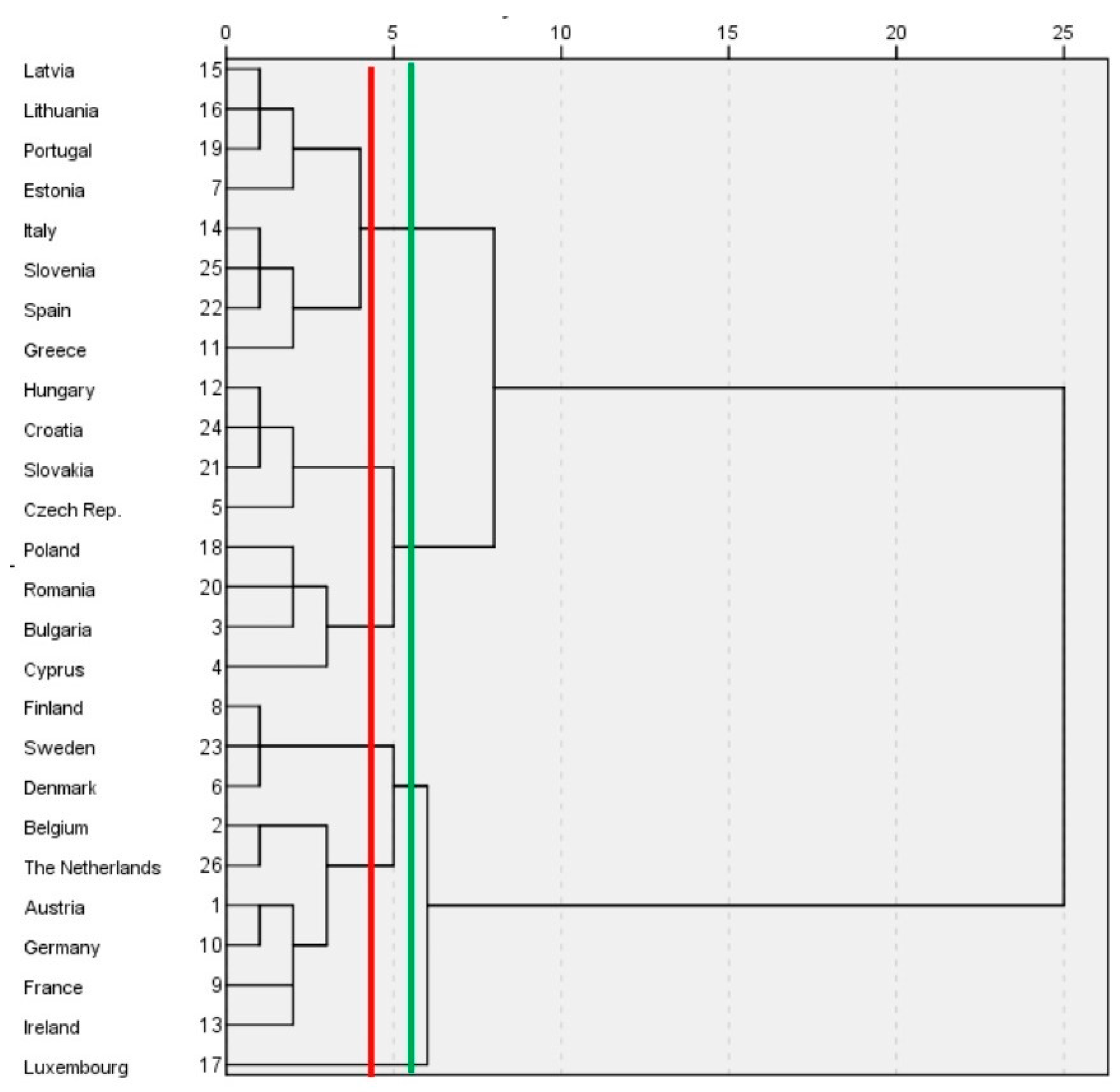
The hierarchical analysis (Figure 1) shows us that the ideal number of clusters is seven. So, using the non-hierarchical method, we will test whether the hypothesis of seven clusters is confirmed or whether it would be better if we split the countries into five clusters, in other words, which solution is more homogeneous. Although not fully visible in the dendrogram, considering six clusters may also be the best solution.

As we mentioned below, it is necessary to understand the ideal number of clusters that we should divide our global sample into. One way to use it is the cluster validation technique. There are currently about a dozen of these techniques; in our specific case, we will use the MaClain Rao index and the Davies–Bouldin index.

The following formula should be used to choose the appropriate number of clusters (Equation (10)):

$$MRI= \frac{\frac{Sw}{Nw}}{\frac{Sb}{Nb}}=\frac{Nb}{Nw}\times \frac{Sw}{Sb}$$

(10)

where Sw/Nw is the average of the sum of the distances within the clusters, divided by the value of distances between pairs that belong to the same cluster; Sb/Nb is the average of the sum of the distances between clusters, divided by the value of the distances between pairs that do not belong to the same cluster. The number of clusters to be considered should be the one with the lowest index value. In other words, the index is calculated by dividing the average of the distances within the cluster and the average distances between clusters.

Additionally, based on the dispersion within the clusters and the separation between them, it has been argued that the adequate number of clusters that we must consider is given by Equation (11):

$$DBI= \frac{1}{n} {\displaystyle \sum }_{i=1}^n\max (\frac{d_i+d_j}{d\left(c_i, c_j\right)})$$

(11)

where n is the number of clusters,$d_i$ and $d_j$ are averages of the distance of all members of each cluster to the respective center and $d\left(c_i, c_j\right)$ is the distance between the centers of the clusters. According to these authors, one should opt for the smallest result, as this is the condition for obtaining a compact cluster with centroids well separated.

As we can see in

Table 9. Cluster validation.

Clusters	McClain Rao	Davies–Bouldin
5	0.32138	0.0064
6	0.28041	0.0031
7	0.24354	0.0042

Source: Authors’ calculations.

, the adequate number of clusters for the three hypotheses that we tested is six since for seven clusters, the value of the Davies–Bouldin index increases slightly. Despite the fact that the value of the McClain Rao index has decreased to between six and seven clusters, we will adopt the six clusters solution, as this will be the point of inflection of the McClain Rao index.

Given the division into six clusters, each of them will be composed of the following countries:

• Cluster 1—Estonia, Italy, Latvia, Lithuania, Portugal, Spain, and Slovenia.
• Cluster 2—Austria, Belgium, France, Germany, and the Netherlands.
• Cluster 3—Bulgaria and Romania.
• Cluster 4—Cyprus, Czech Republic, Greece, Hungary, Poland, Slovakia, and Croatia.
• Cluster 5—Luxembourg.
• Cluster 6—Denmark, Finland, Ireland, and Sweden.

The analysis of the six clusters solution shows the following (Table 2, Table 9 and

Table 10. Average observations in each cluster.

Cluster	GDPpc	GINI	GCI	HDI	EDB	EPI	GEI
1	28,874	32.57	4.56	0.86	72.05	85.57	46.31
2	43,830	27.87	5.35	0.91	74.33	82.58	64.63
3	18,005	35.30	4.19	0.79	68.01	78.88	28.25
4	26,954	29.02	4.31	0.84	67.19	81.67	40.44
5	95,130	28.81	5.21	0.89	67.38	86.25	58.30
6	46,664	27.21	5.40	0.91	81.39	88.93	72.60

Source: Authors’ calculations.

):

• Cluster one is composed of three countries in the Mediterranean Basin, three Baltic countries, and a country in central Europe. What makes these countries so homogeneous is their proximity around the values of the HDI, EPI, and GCI variables.
• Cluster two is made up of central European countries with high purchasing power. The cluster association occurs not only due to purchasing power but also due to the very similar values of the GCI, HDI, and GEI.
• In cluster three, there are only two countries, which, in addition to being neighbors sharing a border greater than 400 km, are the two countries with the lowest purchasing power in the European Union, adding the fact as well that their HDI, EPI, and GCI values are also very homogeneous.
• In cluster four, five of its seven countries belong to the area of influence of the ex-USSR. These countries have homogeneous values of HDI, EPI, and HDI.
• In cluster five is Luxembourg only, essentially due to the high purchasing power per capita.
• Cluster six is composed exclusively of northern European countries, three of which are Nordic. It is a group of countries with a high per capita income, and it is also the cluster that presents the greatest homogeneity in the variables.

5.2. Individual Estimation for Each Cluster Using the Panel Data Methodology

To choose the performed estimation method (OLS, LSDV, or GLS), we use the following: the F-test, testing the pooled model versus the FE model; the Breusch–Pagan LM test, testing the pooled model versus the RE model; and the Hausman test, testing the RE model versus the FE model. Performing the three statistical tests, the FE model was revealed to be the most appropriate specification to adopt to all clusters. Regarding cluster five, which is composed of only one country, it makes no sense to make estimates. In turn, concerning cluster three, since it is only composed of a few observations, the estimates can be biased, so we will not estimate this cluster either.

After carrying out the three statistical tests to support the choice of the best panel data method to estimate the regressions, we found that only in the regression whose dependent variable is the Gini coefficient, and in cluster six, the most appropriate method is the one that uses the random effects. In the other cases, the most appropriate method proved to be that of fixed effects.

Table 11. Results of the Estimation for Each Cluster.

	Cluster 1		Cluster 2		Cluster 4		Cluster 6
	Ln GDPpc	Ln GINI	Ln GDPpc	Ln GINI	Ln GDPpc	Ln GINI	Ln GDPpc	Ln GINI
Intercept	7.6323 **	5.6993 **	9.3827 ***	1.7154	8.8558 ***	2.9787	9.5657	−2.0041
Ln GCI	1.3019 ***	−0.3157	0.8748 ***	−0.0223	1.5199 ***	−0.7441 *	1.6821 ***	−0.0209
Ln HDI	1.5416	1.1496	1.1684 **	−0.6593	1.3859 ***	0.8040	2.6985 ***	0.4489
Ln EDB	0.1217	0.0397	0.3262 *	0.4583	−0.2546	−0.4689	0.5040	0.2903
Ln EPI	0.0461	−0.2644	0.2298	−0.0635	0.2344	0.7091	−0.9051	1.0542
Ln GEI	0.2406 **	−0.1473 **	0.0914	−0.0263	−0.1037	0.1350	0.1326	−0.1472
R-Squared	0.9886	0.9583	0.9612	0.7937	0.9799	0.9333	0.8723	0.8733
F-test (p-value)	$1.13\times {10}^{-007}$	0.0355	0.0001	0.0078	$9.29\times {10}^{-005}$	0.0020	$2.12\times {10}^{-006}$	0.0117

Note: ***, ** and * denote statistical significance at the 1%, 5% and 10% level of significance, respectively. Source: Authors’ estimations.

shows the results obtained through the estimates for the four referred clusters, according to the methodology referred to in the previous paragraph, in which we regressed the GDPpc and the Gini coefficient according to the five independent variables used in this paper.

5.3. Verification of Endogeneity in the Case of Clusters

As previously done, we also go to the case of the clusters’ estimates to see if in any case there is an infraction of the hypothesis of the exogeneity of the explanatory variables, imposing that the methods used are inappropriate, as well as results presented in Table 11 would be biased and inconsistent. We performed the Hausman test and used the first differences of the GEI variable as a supplementary instrument.

As we can see in all the cases in

Table 12. p-value of the Hausman tests for endogeneity.

	Cluster 1		Cluster 2		Cluster 4		Cluster 6
	Ln GDPpc	Ln GINI	Ln GDPpc	Ln GINI	Ln GDPpc	Ln GINI	Ln GDPpc	Ln GINI
Ln GCI	0.2289	0.0626	0.1034	0.8412	0.0839	0.0215	0.6621	0.0537
Ln HDI	0.0103	0.1472	0.2141	0.8565	0.1475	0.0928	0.3342	0.9507
Ln EDB	0.4448	0.5072	0.4862	0.9753	0.0357	0.0476	0.0679	0.6524
Ln EPI	0.0523	0.0761	0.0619	0.0592	0.3048	0.4889	0.6556	0.4234
Ln GEI	0.9813	0.0081	0.1114	0.1439	0.5153	0.9941	0.2923	0.2434

Source: Authors’ calculation.

, five variables can be considered endogenous, given that the p-value of the Hausman test is less than 0.05, namely, in cluster 1, Ln HDI in the regression model of Ln GDPpc, Ln GEI in the regression model of Ln GINI; in cluster 4, Ln EDB in the regression model of Ln GDPpc, and Ln GCI and Ln EDB in the regression model of Ln GINI. In clusters 2 and 6 there are no endogeneity situations. Since in the same model there are two endogenous variables, in that specific case we must use one more instrument that will be the first differences of the EPI variable. As we can see in

Table 13. p-value of the Sargan tests and F-statistics.

	p-Value Sargan Test to Validate the Instruments						First Stage F-Statistic to Test the Weakness of the Instruments
	Cluster 1		Cluster 4 *		Cluster **
	Ln GDPpc	Ln GINI	Ln GDPpc	Ln GINI	Ln GDPpc	Ln GINI	Cluster 1	Cluster 4 *	Cluster 4 **
GCI	0.3321	0.068	0.2056	0.2203	0.0881	0.1234	24.136	27.655	26.151
HDI	0.1535	0.1363	0.9205	0.0746	0.1848	0.3831	36.753	27.873	27.744
EDB	0.2486	0.1015	0.6368	0.0571	0.5904	0.3015	29.822	23.314	21.955
EPI	0.1697	0.8274	0.5609	0.4789	0.2433	0.5791	31.915	29.015	19690
GEI	0.2925	0.0787	0.5319	0.1282	0.3515	0.4512	1396.4	716.56	128.32

Note: * and ** refer to the use of the GEI and EPI instruments, respectively. Source: Authors’ calculation.

, all instruments used are considered valid and strong.

In general terms, we can see in Table 2 that the European Union countries with the highest per capita income are those with the most favorable indicators in social, economic, environmental, and human terms. Regarding the expected impact of regressions on the GDPpc variable, it will be expected that all variables have positive coefficients since they can contribute to economic growth. Concerning the Gini coefficient, it is expected that the coefficients are negative, as it is expected that they cause a decrease in inequalities in the distribution of income.

5.4. Two-Stage Least Squares Estimation Approach for Clusters One and Four

Table 14. Estimation results—2SLS.

	Cluster 1		Cluster 4
	Dependent Variable		Ln GDPpc	Ln GINI
	Ln GDPpc	Ln GINI
Intercept	7.59922 **	1.67885	15.6494	15.1427
Ln GCI	1.30321 ***	0.46627	1.4726 **	−1.9551
Ln HDI	1.52906 **	−1.55092 ***	3.1562 ***	1.4217
Ln EDB	−0.12092	0.61478	−0.5006	−3.4638
Ln EPI	0.05154	−0.19662	−1.1420	1.2317
Ln GEI	0.24106 ***	−0.23614 ***	0.0833	0.2983
Wald chi-Squared (p-value)	0.0000	0.0000	0.0000	0.0000
F-test (p-value)	0.0000	0.0000	0.0037	0.0000

Note: *** and ** denote statistical significance at the 1% and 5% level of significance, respectively. Source: Authors’ estimations.

shows the results obtained from the estimation of clusters 1 and 4, using the Two-Stage Least Squares Estimation Approach.

5.5. Cluster Results’ Discussion

In all the estimated models referring to the division into clusters, the coefficients that present statistical significance for levels normally considered show signs following the expected. As we can see in Table 11 and Table 14, about the estimates for the entire sample, there are some differences. As far as economic growth is concerned, in all clusters, there are at least two statistically significant variables.

The Global Competitiveness Index and Human Development Index have statistical significance in all clusters, varying only in terms of intensity, with cluster two being the one that economically benefits least from competitiveness, and cluster six is the one that most benefits in terms of economic growth with human development, being that it is composed only of countries from the North of Europe.

Cluster 2, which is composed of some of the countries with the highest per capita income in Europe, is the only cluster where the variable Ease of Doing Business assumes significance. The ease these countries provide for doing business, by providing a favorable regulatory environment, is contributing to economic growth and the promotion of business facilities tends to impact economic growth [25,30,56,57].

Although in the integral model the EPI variable is statistically significant and thus shows its contribution to the economy, in none of the clusters the same has occurred. This may be due, for example, to concerns that the protection of human health and the environment in the European Union is only promoting economic growth together, and not in more restricted terms. European countries’ joint and global concerns and attitudes towards environmental and sustainability issues are having a greater impact than in more micro terms. Perhaps the European Union’s commitment to sustainable development will be more visible together, as this is a joint concern of all countries [58].

In the division by clusters, it should be noted that only in the countries that are part of cluster 1, and that are mainly the three Baltic countries and the Iberian countries, is that entrepreneurship takes on significance in reducing inequalities in the distribution of income, being included the only variable that can be considered important. In this case, for each 1% rise in the GEI index of the Baltic and Iberian countries, the average inequality in income distribution in this group of countries is reduced by approximately 0.236%.

The only variable that has statistical significance in all clusters is HDI. In all sets of countries, human development plays an important role in the economic growth of countries. The cluster of Northern European countries is the one that has benefited the most from the level of human development. It should be noted that the countries in this cluster have the highest index in the European Union.

Regarding the distribution of income in a more equitable way, in general, the economic growth obtained by these variables is exacerbating inequalities. The only exception occurs in cluster one, in which, in addition to the HDI variable contributing to a fairer distribution, the GEI variable also does that.

As one would expect the division by clusters of the same variables and for the same period of the countries of the European Union leads us to different results and conclusions. The European Union is made up of a group of countries with great economic, social, and cultural differences. There are countries where the bet on human development has already had its effect on the economy and countries where entrepreneurship by necessity emerged as a means of subsistence and not as a means of creative destruction pointed out by Schumpeter.

6. Conclusions

As one of the ultimate objectives of economic policies to achieve growth, policymakers need to understand how progression is important and if respected international indices promote or do not promote such growth. Likewise, it is no less important to know whether the growth of the economy that is being achieved is increasing or decreasing inequalities in the distribution of income. Countries where income inequality is increasing, are countries where discontent increases can create at least social problems.

Important and well-founded conclusions can be drawn for the countries of the European Union. Of the five important concepts under study, we conclude that human development assumes the most important role in the verified economic growth, as in a more equitable and fairer promotion in the distribution of that economic growth.

By improving the level of health provided to its populations as well as investments in improving the quality and quantity of education, among other factors, they will bring economic returns to the economies of the European Union (seen globally), even though it will cause a decrease in inequalities in income distribution. In terms of the division into clusters, it is worth noting the high importance that human development represents in reducing inequalities in cluster one countries, which alone are some of the European Union countries that present the highest inequalities.

We would like to highlight the value of 2.69 that human development presents in cluster 6, which is composed of the countries of Northern Europe and which are always at the top of the HDI ranking. Perhaps part of its high economic development comes from concerns about human development itself.

Competitiveness also assumes high importance in this study, both for the countries and for all the clusters considered, thus corroborating many of the studies carried out, even for countries of the European Union. A country considered competitive vis-à-vis the players, manages to demonstrate its advantages over the others, in addition to benefiting its entire economy from that same competitiveness. Sectors considered to be less competitive can acquire competitiveness as a result of more competitive ones.

Regarding the positive effects of entrepreneurship on economic growth, its importance is revealed in the integral model and cluster one. Entrepreneurial mindsets bring innovation and their effects spill over to the entire economy, allowing not only to boost economic growth but also the development of the economy.

A favorable regulatory business environment only assumes significance in the cluster composed entirely of some of the countries with the highest income in the European Union, which in itself can demonstrate the importance of this variable on economic growth. Failure to promptly lift legal and bureaucratic barriers can cause investment losses to other countries. Countries with greater facilities in this regard benefit from this, while still controlling their economic activity.

Concerns about sustainability and the environment represent total economic growth in the sample. This result may mean that it is possible to achieve growth without neglecting sustainability. Although some authors mention that these two positions cannot be reconciled, in the European Union economic growth can be achieved without neglecting the planet and future generations, through technological progress and innovation [59].

Because of the results obtained both for the countries as a whole and for the groupings individually, we recommend European Union policymakers pay special attention to the promotion of human development and competitiveness, without neglecting incentives for entrepreneurship. They must also eliminate unnecessary procedures for business activity and remove obsolete and often contradictory legislation.

The European Union, despite being a strong and cohesive economic bloc, is still subject to competition from globalization and from markets that are becoming more and more efficient and competitive.

For future work, it might be interesting to try to understand if these conclusions hold for other geographies or other realities, for example, ASEAN (Association of Southeast Asian Nations) or Asian countries, which are known for their competitive and aggressive profiles in international trade, even if results could be contradictory to those here presented for the European Union countries due to their different profiles and realities. Following the methodology of creating convergence clubs and dividing countries according to their level of income recommended by the World Bank, examining the convergence process based on these five international indicators on different realities could provide insightful policy implications. Another suggestion for future work is to apply the Bayesian Dynamic Factor Model to these data and compare the results obtained.