Abstract
In most cities, discretionary passenger transport by car is predominantly supplied by taxi services. These services face competition from new digital platforms (UBER, Cabify, etc.) that connect users with the services offered by authorized drivers with a license for rented vehicles with drivers (VTC). However, very little is known about the impacts that these services produce in cities where they operate. So far, most studies on this issue have focused on cities of the United States of America, and they broadly found a positive impact in terms of road safety. Road safety has become one of the priority focuses for ensuring social welfare, to the point of being integrated into the Sustainable Development Goals as a primary value to achieve sustainable, safe and responsible mobility. Within this context, the objective of this paper is to analyze the impact of ride-hailing platforms on the frequency of traffic accidents with at least one fatally or seriously injured person in the municipality of Madrid from 2014 to 2018. To do this, a regression analysis has been carried out using a random effects negative binomial regression (RENB). The results of the model show that Uber and Cabify services are associated with a decrease in fatal and serious accidents in Madrid.
1. Introduction
The extraordinary progress in the field of Information and Communication Technologies (ICT), especially with regard to the internet (access to the network and the development of its potentialities), has reconfigured the way people access information, the way they offer goods and services, and ultimately, the way in which people communicate [1,2,3]. These important advances, in conjunction with the increase in the speed of internet connections, the advent of smartphones and the proliferation of smartphone applications, has profoundly reshaped the mechanisms underlying trade, consumption and social relations. This has given rise to new economic models where technology is enabling new ways to connect and to create share value. These new business models employ collaborative platforms that facilitate that people, often private individuals, offer the temporary use of goods without modifying their ownership (for example, rooms in a house), or the service delivery, in exchange, or not, of a consideration. They facilitate the exchange of underused goods, either by selling them or giving them away for free or by sharing space or time [4]. It is also worth mentioning the critical role played by User Generated Contents (UGC) which provide a framework where service quality ratings by users are available to other potential users [5]. According to the National Markets and Competition Commission, this rapidly evolving phenomenon, known as the collaborative economy, has experienced exponential growth in recent years and has enormous future potential, mainly due to the predisposition of the new generation, the digital native, to trust these exchange and production systems, revealing a public and stable identity in digital platforms and ecosystems. Among the top 25 sharing economy platforms worldwide, Uber stands out, with an investment of more than USD 6 billion [6] and has gained such a notoriety that it is frequent to hear terms such as “ubernize” or “uberization” to refer to platforms that, thanks to the internet, allow some people to make availble to others various goods and services.
This platform offers urban and interurban transport solutions, and is based on contacting, through its mobile application, available vehicles and users who demand, instantly, short-distance urban transport within the town. These new services offer an alternative to the service traditionally offered by the taxi sector. However, very little is known about the impact that these ride-hailing services have on the cities where they operate.
In terms of road safety, most of the studies have focused on cities of the United States where these types of services operate. However, these studies have found mixed results with respect to their effects. Meyer asserts in his book that, according to a report issued by Uber and Mothers against Drunk Driving (MADD), young people prefer to use this service rather than driving their own vehicles if they plan to consume alcohol. The results of the study are compatible with other data: after the UberX service began operating in cities in California, the monthly accidents related to alcohol dropped by 6.5% among drivers under the age of 30 [7]. A study on California found that the advent of UberX resulted in a 3.6–5.6% decrease in the rate of motor vehicle homicides per quarter [8]. Morrison et al. [9] found a relationship between the 62% reduction in the accident rate related to alcohol and the implementation of ride-hailing platforms in the city of Portland (Oregon), but not other three cities considered in the study. In the case of New York, a reduction from 25–35% (around 40 collisions per month) was observed in the collision rate related to alcohol in the districts of Manhattan, Bronx, Brooklyn and Queens [10].
On the contrary, and after analyzing data on traffic accident causalities associated with alcohol consumption in the 100 largest metropolitan areas of the United States between 2005 and 2014, no relationship was found between these deaths and the implementation of these services [11]. Similarly, Huang et al. [12] analyzed data for some South African cities and found no evidence of reduction in accident rate after the introduction of Uber.
Road crashes represent today a problem of high economic and social impact. In economic terms, the annual cost of road crashes in the European Union is 2% of its Gross Domestic Product (GDP) [13]. In social terms, because it is one of the leading causes of death globally in children and young people; every 30 s somebody dies in a road crash [14]. So much so that the 2030 Agenda for Sustainable Development has set two goals: target 3.6, which says “by 2020, halve the number of global deaths and injuries from road traffic accidents”, and target 11.2 that says “by 2030, provide access to safe, affordable, accessible and sustainable transport systems for all, improving road safety, notably by expanding public transport, with special attention to the needs of those in vulnerable situations, women, children, persons with disabilities and older people” [15].
Based on this and studies carried out in the United States, ride-hailing platforms such as Uber or Cabify (the principal competitor of Uber in Spain, with cheaper services than taxi) could improve the supply to segments of demand that previously had greater difficulty accessing taxis or public transport, for example in low-income families or residents of the periphery of the cities, and may serve to reduce deaths and serious injuries from traffic accidents.
The aim of this study is to investigate whether there has been a reduction in the rate of accidents during weekend and public holidays and accidents related to alcohol or drug consumption in the municipality of Madrid since the implementation of Uber and Cabify.
2. Materials and Methods
To analyze the impact of ride-hailing platforms on traffic accidents in Madrid, the authors had to face two main challenges.
Firstly, to carry out an in-depth analysis of the accidents that occurred between 2014 and 2018. During these years, a total of 4506 accidents with a fatal or serious injury were recorded, with 43% (1942) of these accidents taking place during weekends or public holydays, and 6.5% (293) of them being related to alcohol or drug consumption (Figure 1).
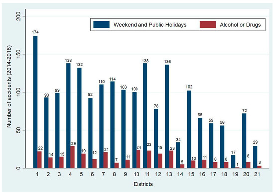
Figure 1.
Distribution of the total number of road accidents (left bars) and accidents related to alcohol consumption recorded during weekend and public holidays in each district of Madrid over the period spanning 2014 through 2018. Source: own research.
Conversely, in a big city like Madrid, with more than 3 million inhabitants, there are large geographical contrasts. Madrid has historically been crossed by a running edge that goes from the north to the south and from the east to the west. In the east and the south, there are industrial areas and traditional working-class neighborhoods, and the north and the west are inhabited by by middle and upper classes. The districts, with their neighborhoods, seem like small independent cities in which there are a main street, where the textile and fast-food franchises are located, parks, squares… and they have their own customs and traditions. For this reason, it was necessary to analyze performance by districts. It is worth highlighting that in this type of analysis which focuses on smaller zones such as wards, neighborhoods or intersections among others, certain variables exist, and some estimation methods are difficult to conduct [16,17,18]. Nevertheless, a small-scale analysis can reveal other effects which are difficult to assess in a wider area analysis [19].
To assess the impact of Uber and Cabify, along with the evolution of other socio-economic factors on the rate of road accident, we carried out a spatio-temporal analysis to compare the accident rate before and after the implementation of Uber and Cabify in the city of Madrid.
2.1. Division of the Municipality by Districts
We decided to analyze the accident rate by district in order to establish a relationship, if any, between the frequency of road accidents and urban areas where they occur, each with its own urban, socio-economic and cultural characteristics.
Dumbaugh and Rae [20] studied how urban form—specifically land use and street network configurations—may influence the incidence of traffic-related crash injuries and deaths. They detailed the development of a database of crash incidence and urban form at the block group level for the City of San Antonio (Texas, USA), the first database of this kind. They analyzed factors such as road infrastructure, urban design, population density or land use at a neighborhood level. They reported a positive association between the presence of arterial or primary roads and road accidents. In addition, they found that specific types of commercial land uses, such as big box stores, are related to a higher risk of accidents. Based on the geospatial analysis proposed by Dumbaugh and Rae, the municipality of Madrid is divided into the 21 districts of which it is made up (Figure 2). In this way, the unit of analysis is the district and not the individual street or location of the accident [18].
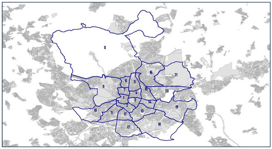
Figure 2.
Map of the 21 districts of Madrid. Source: own research. 1—Centro; 2—Arganzuela; 3—Retiro; 4—Salamanca; 5—Chamartín; 6—Tetuán; 7—Chamberí; 8—Fuencarral-El Pardo; 9—Moncloa-Aravaca; 10—Latina; 11—Carabanchel; 12—Usera; 13—Puente de Vallecas; 14—Moratalaz; 15—Ciudad Lineal; 16—Hortaleza; 17—Villaverde; 18—Villa de Vallecas; 19—Vicálvaro; 20—San Blas-Canillejas; 21—Barajas.
2.2. Traffic Accidents Data Collection
The City Council of Madrid regularly publishes road accident data of the city produced by the Municipal Police between 2010 and 2020 [21]. Each file includes a record for each person involved in an accident (driver, passengers, pedestrians, witnesses, etc.), the type of accident (double collision, multiple collision, pedestrian impact, etc.), the time of the accident, district, street, the meteorological factors and the harm caused. In order to classify the victims in a traffic accident, the methodology of the Spanish Statistical Service of the Directorate-General for Traffic (DGT) has been followed, which categorizes a traffic accident victim as being slightly injured when the person only requires the assistance of emergency services or hospital treatment for less than 24 h, seriously when the victim needs hospitalization for more than 24 h and as fatal victim the person who, as a result of the accident dies at the scene of in the following 30 days [22].
As discussed at the beginning of this paper, traffic accidents are one of the leading causes of death in the world and traffic accidents injuries have become a public health problem [23]. The principal risk factor is alcohol consumption. In low-income countries, between 33% and 69% of the drivers who die in traffic accidents had consumed alcohol [24,25]. For this reason, it was decided to collect traffic accidents with at least one serious injury or fatality in each district of Madrid. In an initial analysis, the dependent variables were divided into two separate groups. The first group included the traffic accidents with at least one seriously injured person and the second the traffic accidents with at least one fatality. Finally, and given that in several districts there had been no accidents with fatal victims, we decided to consider a single group made up of the sum of the accidents with at least one death or serious injury in each district. The two dependent variables measured for each of the 21 districts are listed below:
- Number of accidents at the weekends and public holidays;
- Number of accidents with alcohol or drugs.
For the case of traffic accidents occurring during weekends, we have considered the accidents taking place from Friday at 00:00 to Sunday at 23:59. We also considered the local and national public holidays due to an increase in alcohol consumption [26].
In order to classify the alcohol-related accidents, it was necessary to cross-reference the road accident information obtained from the Statistical Service of the Directorate-General for Traffic (DGT) [27] with that reported by the Municipal Police of Madrid which enabled us to obtain relevant information for each accident such as the district where it occurred or whether those involved had consumed alcohol or drugs.
2.3. Modeling Urban Traffic Accidents
Count data consist of non-negative integer values and are encountered frequently in the modeling of transportation-related phenomena. These data are properly modeled by using a number of methods, the most popular of which are Poisson and negative binomial regression models. Poisson regression is the more popular of the two, and is applied to a wide range of transportation count data [28]. However, there are situations in which observed count data do not meet all of the assumptions of the Poisson regression model. One of the most commonly situations encountered in practice is the individual counts may exhibit more variability than is expected from the Poisson model. Recall that the Poisson distribution has one parameter λi, which characterizes both the mean and the variance of the distribution. Thus, the Poisson model assumes that the conditional mean and variance are equal, a condition known as equidispersion. The situation in which the variance is larger than the mean is known as overdispersion [29].
A number of previous studies pointed out that the crash data are significantly over dispersed [30,31]. This occurs for two primary reasons in cross sectional data. First, there may be individual differences in responses that are not accounted for by the regression model. This problem commonly occurs if an important predictor is omitted from the model. Second, each count that occurs for an individual may not be an independent event as is assumed by the Poisson distribution. This situation is known as contagion or state dependence. In addition, one shortcoming of the Poisson regression model is that it does not contain an error (disturbance) term that fully parallels the error term found in an ordinary least squares (OLS) regression equation. Often there is additional heterogeneity between individuals that is not accounted for by the predictors in the model and the Poisson error function alone, which results in overdispersion. This can overcome by introducing the negative binomial model accounts for overdispersion by assuming that there will be unexplained variability among individuals who have the same predicted value. This additional unexplained variability between individuals leads to larger variance (than expected by the Poisson distribution) in the overall outcome distribution but has no effect on the mean. This additional variability is conceptually similar to the inclusion of an error term in normal linear regression. The Poisson model assumes that the outcomes for all individuals with the same values on the predictors are samples from a single Poisson distribution with a given mean. The negative binomial model, however, allows the observations of individuals with the same values on the predictors to be modeled by Poisson distributions with different mean parameters [29]. To this end, the negative binomial model uses another standard (although less familiar) probability distribution, the gamma distribution to represent the distribution of means [32]. In the negative binomial model, the error function is a mixture of two different probability distributions, the Poisson and gamma distributions [29].
Greene defines in his paper that a useful way to motivate the model is through the introduction of latent heterogeneity in the conditional mean of the Poisson model [33];
where λi = exp (α + xi’β), xi’ is a vector of covariates for segment i, and βi is a vector of estimable regression coefficients, yi and E[yi|xi, εi] are the observed and predicted number of head-on crashes on road segment i, respectively, and hi = exp (εi) is assumed to have a one parameter gamma distribution, G(θ,θ) with mean 1 and variance 1/θ = k;
After integrating hi out of the joint distribution, we obtain the marginal negative binomial (NB) distribution,
The conditional mean of the outcome, given the values of the predictors, is identical for the Poisson model and the negative binomial model.
E[yi|xi] = λi
In contrast, the conditional variance of the outcome will be larger in the negative binomial model than in the Poisson model. The variance for the negative binomial model is given by;
where k = Var[hi].
Var[yi|xi] = λi [1 + (1/θ)λi] = λi [1 + kλi]
The parameters of the negative binomial model are estimated by standard maximum likelihood methods through maximizing the logarithm of likelihood function (Equation (3)).
The superiority of negative binomial model over Poisson regression model depends on the value of dispersion parameter k. If k is not statistically different from zero, the negative binomial model reduces to the Poisson model [34].
Nevertheless, in this study, temporal analysis has to be included in the modeling. Naznin et al. [35] explain in their paper, that when crash data is collected from n = 1, …, N locations for t = 1, …, T time periods, as in our case, the negative binomial model assumes that there are N*T independent observations. The time variant nature in crash data is being omitted by the NB model and standard error of estimated coefficients may be underestimated. One way to overcome this limitation is to treat the crash data in a time series cross sectional panel data structure with N location groups and T time periods, and by considering individual effects in the NB model, as suggested by Hausman et al. [36]. Hausman et al. examined both fixed and random definitions of the individual effects and developed random effects (RE) and fixed effects (FE) models. However, fixed effects models do not allow location specific variations, but random effects models consider randomly distributed location specific variations. Shankar et al. [37] identified the random effects negative binomial (RENB) model as being more appropriate for modeling median crossover crash frequencies in relation to geometric and traffic variables in Washington State. Another study by Chin and Quddus [38] used the RENB model to investigate the relationship between crash occurrence and the geometric, traffic and control characteristics of signalized intersections in Singapore. Both of the studies have found the RENB model suitable for the variables (i.e., geometric and traffic) which are likely to have location specific effects. Moreover, from an analytical viewpoint, RENB models offer advantages in terms of model transferability and updating [28,36,39].
In light of the above, the model that is the most appropriate, and therefore selected for this study is random effects negative binomial (RENB), as available crash data has a panel structure, and the variables are likely to have location specific effects.
The structure of the RENB model used in this study is as follows:
where E(Yit) represents the expected number of accidents in the ith district in year t, Xit is the vector of explanatory variables, β is the vector of regression parameters, εit is the vector of residual errors, ui represents the random effect for the ith location, and exp(ui) is gamma distributed with mean 1 and variance αi, where αi is the parameter of overdispersion in the negative binominal model. The RENB model allows the overdispersion parameter to vary randomly from district to district, such that 1/(1 + αi) follows a Beta (r, s) distribution [35,36,37].
E(Yit) = exp (βXit + ui + εit)
2.4. Variables Analysis
In order to determine the period of analysis for this research, it is necessary to know when Uber and Cabify began operating in Madrid.
Uber arrived in Madrid in September 2014 through its UberPop version which enabled anyone of legal age and with a driving license to register as a driver on the platform, and provide transport services at the request of the users. This service was only in operation until December 2014, when Madrid Mercantile Court Nº. 2 ordered the precautionary suspension of the service throughout Spain alluding to “the nature of the commercial service provided by Uber, its cross-border vocation, its will to sequentially gain a strong position in the passenger transport market without fulfilling the administrative requisites”. After the precautionary suspension of its activity, in March 2016 Uber returned to Madrid, changing its model to adapt to the legislation in force. In this way, since then Uber has been operating using professional drivers (self-employed or companies) with a VTC license. Until then, Cabify has been operating in Madrid since 2011.
It would be logical to consider years prior to 2014 for this study, 2016 has been considered as the first year in which these services have been operating in the city of Madrid. This is because between January 2000 and September 2015, according to the National Commission on Markets and Competition, a global investment in initiatives related to the sharing economy was calculated to amount to 25,972 million dollars. But this investment was particularly noteworthy between 2013 and 2015, since it grew from 1820 million dollars (2013) to 12,890 million dollars (2015), of which, 62% was invested in transport related models [5]. In the case of Spain, the companies managing the ride-hailing platforms of Uber and Cabify also recorded a considerable increase in their revenue from the year 2015 (Table 1) [40].

Table 1.
Evolution of Uber and Cabify income in Spain. Source: own research.
With respect to licenses for rented vehicles with drivers in the Region of Madrid, which are necessary for these platforms to operate, we can observe a rapid growth from 2015 (Figure 3), with this growth being particularly prominent in 2018 and 2019 [41,42].
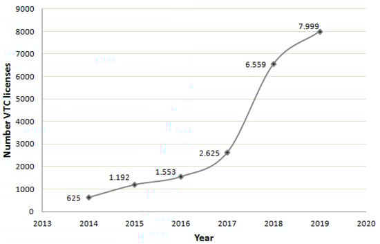
Figure 3.
Evolution of rental vehicles with driver (VTC) in the Region of Madrid. Source: own research.
Therefore, the period of analysis chosen for this research is 2014–2018. To indicate the presence of Uber and Cabify during the years of study, a binary variable has been used with value 1 and 0 indicating the presence and absence of the service, respectively.
It should be noted that more than 90% of fatal crashes occur in low-income and middle-income countries (LMIC). Even in high-income countries, people of lower socio-economic status are most at risk of being involved in these types of accidents [14]. For this reason, we had to include a variable of socio-economic status. This variable is an indicator that is calculated based on the average income per household and district (Equation (6)), following the methodology used in the report conducted by the Area of Government of Territorial Coordination and Public-Social Cooperation of Madrid for calculating the territorial vulnerability index of neighborhoods and districts of Madrid and the vulnerability ranking [43]. The annual average income values have been drawn from the “Urban Audit” conducted by the Spanish National Statistics Institute (INE) [44]. In this case there were no data available referring to income per household for the year 2017 and this was estimated using the Consumer Price Index (CPI of Madrid for that year).
where:
Per capita income is one of the indicators most used in vulnerability and social exclusion studies.
The economic well-being of people can be assessed more precisely when focusing on the part of national income that is directly related to households, that is, the disposable income, consumption expenditure and net savings added to the portion of public spending related to health, education, housing, the environment and social welfare [45]. To do this, average family income is a more reliable indicator as it contemplates not only the individual incomes of the households, but it analyzes them from a comprehensive perspective of a group of people who make common economic decisions, share their income and make a series of expenditures that equally benefit all of the members of the group [46].
Most of the research on poverty in developed countries focuses on household income as the most solvent instrument to capture standards of living and distinguish those who live in a vulnerable situation from those who have a level above the average. As well as analyzing how many of these households are at risk of poverty, it is not only able to capture the resource deprivation that puts the people living in the household at risk, but it is also able to identify and relate it to different groups of households [47].
It has also been considered relevant to take into account the number of leisure establishments in each district as points of attraction for drivers, particularly at weekends and on public holidays. These data have been obtained from the census of premises and activities that the City Council of Madrid publishes in its open data bank. Another variable included is the total size of the population in each district per year of the study.
It is worth noting that during the years analyzed there were no significant changes in the traffic regulations or the sanctions for improper driving, so the study does not include legislative variables.
Three different statistical models have been generated, comparing each one of the three dependent variables against all of the independent variables in order to find spatial relationships between socio-economic and urban factors, ride-hailing services and traffic accidents. These two models are as follows:
- Accidents at the weekends and public holidays (Model 1);
- Accidents with alcohol or drugs (Model 2).
Table 2 shows a summary of the variables considered in this analysis.
Table 2.
Variables. Source: own research.
Before inclusion of variables into the model, a correlation matrix was developed to examine whether the variables of concern are highly correlated with other variables. The basic idea was to avoid inclusion of both variables which were highly correlated. Correlation among variables were tested depending on the Pearson’s correlation coefficient. The correlation was considered as high when the coefficient was more than ±0.7 [35,48,49].
2.5. Model Goodness of Fit and Selection
Model goodness of fit was tested and compared using the McFadden [50] pseudo-R-squared value, estimated as follow:
where LL(β) is the log-likelihood value of the full model, and LL(C) is log-likelihood value of the constant only model.
In addition, two information criteria were used to compare both models: the Akaike information criterion (AIC) and the Bayesian information criterion (BIC). The AIC and BIC are defined as follows:
where LL is the logarithm of the maximum likelihood estimation for each model, P is the number of model parameters, and n is the number of observations (n = 105).
A model with the lowest AIC and BIC values is preferred. To decide whether there is a statistically significant difference between two models, Hilbe’s AIC and Raftery’s BIC rule-of-thumb criteria were adopted in this study [51,52].
Table 3 shows the significance levels for both criteria.
Table 3.
Significance levels for AIC and BIC. Source: Raftery, 1995 and Hilbe, 2011.
In this case study (n = 105), if the difference in the AIC value is greater than 6.0, then the model with lower AIC is favored over another.
3. Results and Discussion
As previously mentioned, the study was conducted using data corresponding to the period between 2014 and 2018. Table 4 provides a brief description and summary statistics about the variables used in crash frequency model for the present study. Key features of the input are:
Table 4.
Descriptive statistics. Source: own research.
- The mean and standard deviation for accidents at the weekends and on public holidays research 18.50 and 8.96 respectively; and accidents with alcohol or drugs involved, 2.79 and 2.57, respectively. These numbers imply that a NB regression model is more suitable than a Poisson regression model;
- The average population is 152,670 inhabitants per district, but the ratio of population goes from a minimum of 45,950 to a maximum of 253,430 inhabitants;
- Madrid has an average of 860 leisure establishments per district;
- The indicator of socio-economic status has a mean value of 4.76 per cent.
Table 5 presents the matrix of the Pearson’s correlation coefficients among all variables considered for the model. The results show that none of the variables are highly correlated with other variables as the correlation coefficients are less than ±0.7.
Table 5.
Pearson’s correlation coefficients among variables. Source: own research.
The dispersion parameter estimated from the NB model was found to be significantly different from zero, which suggests that the negative binomial model structure was more suitable than the Poisson structure.
Table 6 presents the comparison results for random effects negative binomial (RENB) and the negative binomial (NB) models. To develop and select the considered models, the statistical software package STATA version 16 was used. The results show that the RENB model results in a significantly better log-likelihood at convergence than the NB model. Moreover, the RENB model improves overall fit (R2 = 0.17 Model 1 and R2 = 0.14 Model 2) compared to the NB model (R2 = 0.15 Model 1 and R2 = 0.12 Model 2). The likelihood-ratio test vs. pooled test result indicates that the panel estimation is significant compared to the pooled estimation.
Table 6.
Results of the fitted models. Source: own research.
The two information criteria (AIC and BIC) are also used to determine the best model. Both AIC and BIC give advantage to the RENB model over NB. In terms of AIC, the RENB model has the lowest value. Based on Hilbe’s rule-of-thumb for this study (n = 105), if AIC is greater than 6.0, then the model with the lowest AIC is preferred. For this study sample, the difference in AIC was found for RENB versus NB by nearly 14, in model 1 and 6.15 in model 2, therefore the RENB is strongly preferred over NB. The superiority of the RENB model was also supported by the BIC. Based on Raftery’s rule-of-thumb, the BIC was found to be very strong for the RENB versus NB by 12 in Model 1 and positive difference in Model 2, which favors the random effect model.
In addition, the Hausman specification test is insignificant, which suggests using the random effects model instead of the fixed effects model.
The results of RENB model is presented in Table 7. In the case of the city of Madrid, the variable of rail-hailing services has a negative coefficient and is statistically significant in two models, meaning that the implementation of Uber and Cabify has reduced accidents with at least one fatal or seriously injured victim. Moreover, in accordance with Meyer [7] and Greenwood & Wattal [8], accidents related to alcohol and drugs have also reduced in the years since Uber and Cabify have been operating.
Table 7.
Results of the estimated Model (z-statistics in parentheses). Source: own research.
With respect to the influence of the population on traffic accidents, this variable is also statistically significant with a positive coefficient in the two models, which shows that a higher level of population generates more traffic and, as a result, gives rise to an increase in traffic accidents, in the same way as in the study carried out by Casares et al. [19].
Socio-economic status variable is significant and has a negative value in the case of Model 1 which means that since Uber and Cabify began operating, accidents occurring at the weekend and on public holidays with seriously injured or fatal victims have fallen in the most vulnerable districts. As mentioned at the beginning of this article, the most vulnerable areas are more prone to suffering accidents with fatalities. However, the impact of this variable for accidents related to alcohol is not significant and, therefore, cannot be considered as being conclusive data for this study.
With respect to leisure establishments, this variable has a positive coefficient in the two models and is also significant, which means that there is a close relationship between the local leisure agglomerations (restaurants, pubs, theaters, cinemas, etc.) and a higher concentration of accidents with seriously injured or fatal victims.
However, we must acknowledge that this study has certain limitations. First, we do not have information about the individual use of Uber or Cabify, therefore, we cannot analyze the direct relationship between these services and the accidents with seriously injured or fatal victims in the different districts, as we do not know in which districts Uber and Cabify have a greater presence.
Second, we know the district where the accident occurs but the victim of the fatal or serious accident does not necessarily have to reside in that district. The traffic accident could have happened during the course of the journey. For this reason, we cannot relate the reduction in the accidents in the most vulnerable districts with the reduction of deaths per traffic accident in people with a lower socio-economic level and with a greater risk of being involved in these types of accident.
Finally, the study does not examine the relationship of the ride-hailing services in traffic accidents with young drivers and traffic accidents with young drivers under the influence of alcohol. In future research it would be advisable to analyze these relationships to confirm whether young people do actually prefer to use these types of service when they plan to go out and drink alcohol.
In spite of these limitations, this study complements the research carried out in cities in the United States and obtains the first results of the relationship between ride-hailing services and urban accident rates in the municipality of Madrid.
4. Conclusions
The disruption caused by these platforms and their effects on urban mobility, urban development or infrastructure planning are still not definitive, although the available studies have, in general, obtained positive results in those cities that have more experience in the provision of these services.
The findings of this analysis reveal that the implementation of Uber and Cabify services in the city of Madrid is related to a reduction of accidents with seriously injured or fatal victims at weekends and on public holidays, as well as in accidents related to alcohol and drugs.
This study shows that these services have had a positive impact on the most vulnerable districts, reducing accidents on weekends and on public holidays, but it is not significant in the case of accidents related to alcohol. Furthermore, similarly to the presence of leisure establishments, the population has a significant impact on the concentration of traffic accidents. This result coincides with that described in the book by Meyer, which indicates that the entrance of these new competitors gives rise to an increase in the supply which can make these types of services more accessible to a segment of demand which has difficulty accessing taxis. When the number of vehicles is lower, they tend to be concentrated in central areas of the city where the demand is higher. Furthermore, the ride-hailing services have dynamic prices which vary depending on the demand for drivers, for example, at Halloween or on New Year’s Eve, where the tariff can be up to three times higher. This increase in prices encourages more drivers to work at times of high demand and the users to trust in a service that will guarantee their return home after a night out, even if they live in the outskirts of the city [6], reducing the need to use private vehicles to go out, and thus contributing to a reduction of accidents related to alcohol.
Author Contributions
Conceptualization, M.F., A.O., B.G. and J.C.; methodology, M.F., J.C.; software, M.F., J.C.; validation, M.F., A.O., B.G. and J.C.; formal analysis, M.F.; investigation, M.F; resources, M.F.; data curation, M.F.; writing—original draft preparation, M.F.; writing—review and editing, M.F., A.O., B.G. and J.C.; visualization, M.F.; supervision, M.F., A.O.; project administration, A.O.; funding acquisition, M.F. All authors have read and agreed to the published version of the manuscript.
Funding
María Flor García is currently developing her doctoral thesis on sharing economy and mobility and she enjoy an FPU grant from the University of Alicante.
Institutional Review Board Statement
Not applicable.
Informed Consent Statement
Not applicable.
Data Availability Statement
Publicly available datasets were analyzed in this study. This data can be found here:
- Traffic accidents in the City of Madrid: https://datos.madrid.es/portal/site/egob/menuitem.c05c1f754a33a9fbe4b2e4b284f1a5a0/?vgnextoid=7c2843010d9c3610VgnVCM2000001f4a900aRCRD&vgnextchannel=374512b9ace9f310VgnVCM100000171f5a0aRCRD&vgnextfmt=default# (accessed on 28 December 2020)
- VTC licenses evolution: https://www.mitma.gob.es/transporte-terrestre/servicios-al-transportista/observatorios-del-transporte/observatorios-del-transporte-de-viajeros-por-carretera (accessed on 2 September 2019); https://www.mitma.gob.es/transporte-terrestre/servicios-al-transportista/observatorios-del-transporte/observatorios-del-transporte-de-viajeros-por-carretera (accessed on 2 September 2019)
- Average income per household; https://www.madrid.es/portales/munimadrid/es/Inicio/El-Ayuntamiento/Estadistica/Areas-de-informacion-estadistica/Economia/Renta/Urban-Audit/?vgnextfmt=default&vgnextoid=6d40393c7ee41710VgnVCM2000001f4a900aRCRD&vgnextchannel=ef863636b44b4210VgnVCM2000000c205a0aRCRD (accessed on 1 April 2020)
- Leisure Establishments; http://www-2.munimadrid.es/CSE6/control/seleccionDatos?numSerie=4020400031 (accessed on 20 March 2020)
- Population; http://www-2.munimadrid.es/TSE6/control/seleccionDatosBarrio (accessed on 20 March 2020)
A part of the accident data used in this study (accidents with alcohol) has been requested from the General Directorate of Traffic since these data are not publicly.
Conflicts of Interest
The authors declare no conflict of interest.
References
- Botsman, R.; Rogers, R. What’s Mine is Yours—The Rise of Collaborative Consumption; HarperCollins e-Books: New York, NY, USA, 2010. [Google Scholar]
- Guillén Navarro, N.A.; Iñiguez Berrozpe, T. Public action and collaborative consumption. Regulation of tourist accommodation in the P2P context. Pasos 2016, 14, 751–768. [Google Scholar] [CrossRef]
- Zervas, G.; Proserpio, D.; Byers, J.W. The Rise of the Sharing Economy: Estimating the Impact of Airbnb on the Hotel Industry. J. Mark. Res. 2017, 54. [Google Scholar] [CrossRef]
- Méndez, M.T.; Castaño, M.S. Keys to the collaborative economy and public policies. Econ. Ind. 2016, 402, 11–17. [Google Scholar]
- Owusu, R.A.; Mutshinda, C.M.; Antai, I.; Dadzie, K.Q.; Winston, E.M. Which UGC features drive web purchase intent? A spike-and-slab Bayesian Variable Selection Approach. Internet Res. 2016, 26, 22–37. [Google Scholar] [CrossRef]
- National Commission for Markets and Competition. Study on New Service Provision Models and the Collaborative Economy—E/CNMC/004/15; Comisión Nacional de los Mercados y la Competencia: Madrid, Spain, 2016. [Google Scholar]
- Meyer, J. Uber Possitive: Why Americans Love the Sharing Economy; Encounter Books: New York, NY, USA, 2016. [Google Scholar]
- Greenwood, B.N.; Wattal, S. Temple University. Show me the way to go home: An empirical investigation of ride-sharing and alcohol related motor vehicle fatalities. MIS Q. 2017, 41, 163–187. [Google Scholar] [CrossRef]
- Morrison, C.N.; Jacoby, S.F.; Dong, B.; Delgado, M.K.; Wiebe, D.J. Ridesharing and motor vehicle crashes in 4 U.S. cities: An interrupted time-series analysis. Am. J. Epidemiol. 2018, 187, 224–232. [Google Scholar] [CrossRef] [PubMed]
- Peck, J. New York City Drunk Driving after Uber: Working Paper 13; City University of New York: New York, NY, USA, 2017. [Google Scholar]
- Brazil, N.; Kirk, D.S. Uber and metropolitan traffic fatalities in the United States. Am. J. Epidemiol. 2016, 184, 192–198. [Google Scholar] [PubMed]
- Huang, J.Y.; Majid, F.; Daku, M. Estimating effects of Uber ride-sharing service on road traffic-related deaths in South Africa: A quasiexperimental study. J. Epidemiol Community Health 2019, 73, 263–271. [Google Scholar] [CrossRef] [PubMed]
- European Comission. Road Safety: Europe’s Roads are Becoming Safer, but Progress is Still Too Slow. Press Release. 11 June 2020. Available online: https://ec.europa.eu/commission/presscorner/detail/es/ip_20_1003 (accessed on 15 July 2020).
- World Health Organization. Global Status Report on Road Safety 2018; World Health Organization: Geneva, Switzerland, 2018. [Google Scholar]
- United Nations. Sustainable Development Goals. Available online: https://www.un.org/sustainabledevelopment (accessed on 15 July 2020).
- Dissanayake, D.; Aryaija, J.; Wedagama, P. Modelling the effects of land use and temporal factors on child pedestrian casualties. Accid. Anal. Prev. 2009, 41, 1016–1024. [Google Scholar] [CrossRef]
- Miranda-Moreno, L.F.; Morency, P.; El-Geneidy, A.M. The link between built environment, pedestrian activity and pedestrian–vehicle collision occurrence at signalized intersections. Accid. Anal. Prev. 2011, 43, 1624–1634. [Google Scholar] [CrossRef]
- Wang, Y.; Kockelman, K.M. A Poisson-lognormal conditional-autoregressive model for multivariate spatial analysis of pedestrian crash counts across neighborhoods. Accid. Anal. Prev. 2013, 60, 71–84. [Google Scholar] [CrossRef] [PubMed]
- Casares, B.; Fernández, F.; Ortuño, A. Built environment and tourism as road safety determinants in Benidorm (Spain). Eur. Plan. Stud. 2019, 27, 1314–1328. [Google Scholar] [CrossRef]
- Dumbaugh, E.; Rae, R. Safe urban form: Revisiting the relationship between community design and traffic safety. J. Am. Plan. Assoc. 2009, 75, 309–329. [Google Scholar] [CrossRef]
- Madrid City Council. Traffic Accidents in the City of Madrid. Available online: https://datos.madrid.es/portal/site/egob/menuitem.c05c1f754a33a9fbe4b2e4b284f1a5a0/?vgnextoid=7c2843010d9c3610VgnVCM2000001f4a900aRCRD&vgnextchannel=374512b9ace9f310VgnVCM100000171f5a0aRCRD&vgnextfmt=default# (accessed on 28 December 2020).
- Directorate-General for Traffic of Spain (Dirección General de Tráfico). Statistical Yearbook of Accidents. 2016. Madrid: Spanish Ministry for Home Affairs. Available online: http://www.dgt.es/Galerias/seguridad-vial/estadisticas-eindicadores/publicaciones/anuario-estadistico-de-accidentes/Anuario-accidentes-2016.pdf (accessed on 20 April 2020).
- World Health Organization. Global Status Report on Road Safety 2015; World Health Organization: Geneva, Switzerland, 2015; Available online: https://www.who.int/violence_injury_prevention/road_safety_status/2015/Summary_GSRRS2015_SPA.pdf?ua=1 (accessed on 20 June 2020).
- World Health Organization. World Report on Road Traffic Injury Prevention; Peden, M., Scurfield, R., Sleet, D., Eds.; World Health Organization: Geneva, Switzerland, 2004. [Google Scholar]
- Wesson, H.K.; Boikhutso, N.; Hyder, A.A.; Bertram, M.; Hofman, K.J. Informing road traffic intervention choices in south Africa: The role of economic evaluations. Glob. Health Action 2016, 9, 30728. [Google Scholar] [CrossRef]
- Anowar, S.; Yasmin, S.; Tay, R. Comparison of crashes during public holidays and regular weekends. Accid Anal. Prev. 2013, 51, 93–97. [Google Scholar] [CrossRef]
- Directorate-General for Traffic of Spain (Dirección General de Tráfico). Statical Service. 2014–2018; Minister for Home Affairs: Madrid, Spain.
- Washington, S.P.; Karlaftis, M.G.; Mannering, F.L. Methods Statistical and Econometric for Transportation Data Analysis; CRC Press: Boca Raton, FL, USA, 2010. [Google Scholar]
- Coxe, S.; West, S.G.; Aiken, L.S. The analysis of count data: “A Gentle Introduction to Poisson Regression and Its Alternatives”. J. Pers. Assess. 2009, 91, 121–136. [Google Scholar] [CrossRef] [PubMed]
- Miaou, S.-P. The relationship between truck accidents and geometric designof road sections: Poisson versus negative binomial regressions. Accid. Anal. Prev. 1994, 26, 471–482. [Google Scholar] [CrossRef]
- Abdel-Aty, M.A.; Radwan, A.E. Modeling traffic accident occurrence andinvolvement. Accid. Anal. Prev. 2000, 32, 633–642. [Google Scholar] [CrossRef]
- Freund, J.E.; Walpole, R.E. Mathematical Statistics, 3rd ed.; Prentice-Hall: Englewood Cliffs, NJ, USA, 1980. [Google Scholar]
- Greene, W. Functional forms for the negative binomial model for count data. Econ. Lett. 2008, 99, 585–590. [Google Scholar] [CrossRef]
- Hosseinpour, M.; Yahaya, A.; Sadullah, A. Exploring the effects of roadway characteristics on the frequency and severity of head-on crashes: Case studies from Malaysian federal roads. Accid. Anal. Prev. 2014, 62, 209–222. [Google Scholar] [CrossRef]
- Naznin, F.; Currie, G.; Logan, D.; Sarvi, M. Application of a random effects negative binomial model to examinetram-involved crash frequency on route sections in Melbourne, Australia. Accid. Anal. Prev. 2016, 92, 15–21. [Google Scholar] [CrossRef] [PubMed]
- Hausman, J.A.; Hall, B.H.; Griliches, Z. Econometric Models for Count Datawith an Application to the Patents-R&D Relationship; National Bureau of Economic Research: Cambridge, MA, USA, 1984. [Google Scholar]
- Shankar, V.; Albin, R.; Milton, J.; Mannering, F. Evaluating likelihoods median crossover with clustered accident counts: An empirical inquiry using the random effects negative binomial model. Transp. Res. Rec. J. Transp. Res. Board. 1998, 1635, 44–48. [Google Scholar] [CrossRef]
- Chin, H.C.; Quddus, M.A. Applying the random effect negative binomialmodel to examine traffic accident occurrence at signalized intersections. Accid. Anal. Prev. 2003, 35, 253–259. [Google Scholar] [CrossRef]
- Lord, D.; Mannering, F. The statistical analysis of crash-frequency data: A review and assessment of methodological alternatives. Transp. Res. Pt. A 2010, 44, 291–305. [Google Scholar] [CrossRef]
- Sistema de Análisis de Balances Ibéricos (SABI). Madrid Informa. Available online: http://www.informa.es/es/soluciones-financieras/sabi (accessed on 3 September 2014).
- Ministry of Transport, Mobility and Urban Agenda. Observatory of Passenger Transport by Road. Supply and Demand. 2014. Available online: https://www.mitma.gob.es/transporte-terrestre/servicios-al-transportista/observatorios-del-transporte/observatorios-del-transporte-de-viajeros-por-carretera (accessed on 2 September 2019).
- Ministry of Transport, Mobility and Urban Agenda. Observatory of Passenger Transport by Road. Supply and Demand. 2019. Available online: https://www.mitma.gob.es/transporte-terrestre/servicios-al-transportista/observatorios-del-transporte/observatorios-del-transporte-de-viajeros-por-carretera (accessed on 2 September 2019).
- Madrid City Council. Methodology for the Preparation of the Territorial Vulnerability Index of Neighborhoods and Districts of Madrid and Ranking of Vulnerability. Available online: https://datos.madrid.es/portal/site/egob/menuitem.c05c1f754a33a9fbe4b2e4b284f1a5a0/?vgnextoid=d029ed1e80d38610VgnVCM2000001f4a900aRCRD&vgnextchannel=374512b9ace9f310VgnVCM100000171f5a0aRCRD&vgnextfmt=default (accessed on 1 April 2020).
- Madrid City Council. Urban Audit. Available online: https://www.madrid.es/portales/munimadrid/es/Inicio/El-Ayuntamiento/Estadistica/Areas-de-informacion-estadistica/Economia/Renta/Urban-Audit/?vgnextfmt=default&vgnextoid=6d40393c7ee41710VgnVCM2000001f4a900aRCRD&vgnextchannel=ef863636b44b4210VgnVCM2000000c205a0aRCRD (accessed on 1 April 2020).
- Jacobs, G.; Slaus, I. Indicators of Economic Progress: The Power of Measurement and Human Welfare. Cadmus. Available online: http://cadmusjournal.org/node/11#HEWI (accessed on 1 April 2020).
- Navarro Rodríguez, S.R.; Larrubia Vargas, R. Indicators to Mediate Situations of Social Vulnerability, Proposal made in the framework of a European Project. Baetica Estud. Arte Hist. Geogr. 2006, 28, 485–506. [Google Scholar]
- Nolan, B.; Whelan, C.T. Using Non-Monetary Deprivation Indicators to Analyse Poverty and Social Exclusion in Rich Countries: Lessons from Europe? The Economic and Social Research Institute: Dublin, Ireland, 2009. [Google Scholar]
- Hinkle, D.E.; Wiersma, W.; Jurs, S.G. Applied Statistics for the BehavioralSciences, 5th ed.; Houghton Mifflin: Boston, MA, USA, 1979. [Google Scholar]
- Mukaka, M. A guide to appropriate use of Correlation coefficient in medical research. Malawi Med. J. 2012, 24, 69–71. [Google Scholar] [PubMed]
- McFadden, D. Conditional logit analysis of qualitative choice behavior. In Frontiers in Econometrics; Zarembka, P., Ed.; Academic Press: New York, NY, USA, 1973. [Google Scholar]
- Hilbe, J.M. Negative Binomial Regression; Cambridge University Press: Cambridge, UK, 2011. [Google Scholar]
- Raftery, A.E. Bayesian model selection in social research. Soc. Methodol. 1995, 25, 111–164. [Google Scholar] [CrossRef]
Publisher’s Note: MDPI stays neutral with regard to jurisdictional claims in published maps and institutional affiliations. |
© 2021 by the authors. Licensee MDPI, Basel, Switzerland. This article is an open access article distributed under the terms and conditions of the Creative Commons Attribution (CC BY) license (https://creativecommons.org/licenses/by/4.0/).