Article

Interrelationships between Land Use Land Cover (LULC) and Human Thermal Comfort (HTC): A Comparative Analysis of Different Spatial Settings

1
School of Architecture, Faculty of Built Environment, Tunku Abdul Rahman University College, Kuala Lumpur 53300, Malaysia
2
Faculty of Architecture and Ekistics, Universiti Malaysia Kelantan, Bachok 16300, Malaysia
3
Faculty of Built Environment and Surveying, Universiti Teknologi Malaysia, Skudai 81310, Malaysia
4
Geoinformatic Unit, Geography Section, School of Humanities, Universiti Sains Malaysia, USM, Pulau Pinang 11800, Malaysia
*
Author to whom correspondence should be addressed.
Sustainability 2021, 13(1), 382; https://doi.org/10.3390/su13010382
Submission received: 9 December 2020 / Revised: 26 December 2020 / Accepted: 30 December 2020 / Published: 4 January 2021

Abstract

:
A few studies on outdoor human thermal comfort (HTC) have been conducted in the tropical region in a hot and humid climate; however, there is a paucity of discussions on how exactly different spatial settings influence HTC. Thus, this paper aims to examine how land use land cover (LULC) affects HTC on the basis of the simulation of Predicted Mean Vote (PMV) and Physiologically Equivalent Temperature (PET) indices via ENVI-met and Rayman. The results reveal that people living in the urban area have a higher tendency to experience strong heat stress (25% of the areas with PMV ranging from 3.4 to 3.9 and 2% of the areas, where PMV reached 4.1), followed by the rural area (43% of the areas with PMV ranging from 2.1 to 2.4), and the suburban area (more than 50% of the areas with PMV values less than 2.4). Surprisingly, a concrete LULC in the suburb area exhibits a higher air temperature than an asphalt surface at 4 p.m., due to the large area of high albedo that increases the reflection of solar radiation, subsequently contributing to warming up the airmass. Similarly, sandy, and loamy LULC tend to emit more heat during nighttime, while the heat is absorbed slowly during daytime, and it is then slowly released during nighttime after 6 p.m. Spatial settings that promote heat stress in the urban area are mainly contributed by an LULC of asphalt, concrete, sandy, and loamy areas. Meanwhile, people in the suburban and rural areas are less likely to experience heat stress, due to agricultural plantations and lowland forest that provide shade, except for the barren lands-loamy areas. The result also indicates that tree-covered areas near the river in the suburban area afforded the best thermal experience with PMV of 2.1 and PET of 30.7. From the LULC comparison, it is pivotal to consider tree species (canopy density), surface material (albedo), sky-view factor, wind direction, and speed toward designing a more comfortable and sustainable environment.

1. Introduction

Rapid urbanization has induced changes in ecological function and processes, where it has significantly impacted ecosystem services [1]. One of the consequences of urbanization is related to climate change as a real and present threat to socio-ecological sustainability on the planet [2]. The increase of heat intensity in urban areas with the rise of the air temperature has a strong connection with the occurrence of heat stroke, hyperthermia, or even death cases, for example, the heat waves that hit China in 1998 and 2003 and France in 2003 [3,4]. One of the best-known effects that changes the atmospheric condition of an urban environment is known as the urban heat island effect (UHI), which makes a difference in temperatures between an urban and a rural environment [5]. Such effects are attributed to the rampant growth and expansion of built-up areas, contributing to heat stored and radiation by urban structures [6]. Hence, the capacity of an ecosystem to reduce the heat through biologically mediated processes is crucial [7]. For instance, there is a plethora of evidence suggesting that vegetation has been playing a crucial role in reducing urban heat (e.g., Bowler et al. [4]; Oliveira, Andrade and Vaz, [8]; Susca et al. [9]; Shishegar, [10]; Kong et al. [11]; Lindén et al. [12]; Zupancic et al. [13]). Trees are vital, serving as a cooling agent mainly through evaporative cooling and shading of the ground; they also reduce the sky-view factor that obstructs solar radiation received at the ground and human body [14]. In addition, they also obstruct and store heat from solar radiation through leaf absorption, transmission, and reflection [15]. Unlike trees, grasses reduce temperatures in urban areas mainly through evapotranspiration at the ground level [16]. Hence, they help to mitigate urban surface temperatures and reduce excess heat in an urban atmosphere [17]. Similarly, Armson et al. [18] posit that grassland has a better cooling effect compared to concrete and asphalt surfaces. More precisely, they suggested that small plot areas (~0.1 ha) of grasslands may provide better cooling than those of large grasslands (~7.8 ha) because some of the solar energy is converted into sensible heat. Aflaki et al. [19] and Wong et al. [20] advocate that the use of green roofs, green facades, and greenery are effective towards mitigating the UHI effect. For example, urban greening on a roof top could reduce the global air temperature up to 4% and mean radiant temperature up to 4.5% [20]. From the literature alone, we can assert that greenery can improve the microclimate condition and indirectly regulate people’s physical and psychological well-being, especially as regards the human thermal comfort (HTC).
HTC is basically assessed on the basis of three major principles, including human heat energy balance, physiology, and psychology [21,22]. As one of the prominent scholars pioneering in HTC studies, Fanger [23] is of the opinion that the relationships between the environmental parameters (air temperature, mean radiant temperature, air velocity, and relative humidity) and the human physiological parameters (metabolic rate and clothing insulation) are significant factors influencing HTC. These parameters have been adopted in the thermal comfort model by Fanger [24], namely the Predicted Mean Vote (PMV), and the thermal comfort model by Mayer and Höppe [25], namely the Physiologically Equivalent Temperature (PET). Generally, there are several indices which can be used to estimate HTC [26], namely Effective Temperature (ET), Standard Effective Temperature (SET), PMV, PET, and Universal Thermal Climate Index (UTCI). Among these, the most common index used today is PET, due to the direct approximation between what is calculated and what people actually feel, which is quite the same [26,27] and a simple comparable unit in degree Celsius [28]. Whereas, PMV, initially developed by Fanger [24] for an indoor setting, has also been modified to suit the outdoor conditions by Jendritzky and Nubler [29], and the model is known as the Klima-Michel Model [26].
There is a growing research trend showing that thermal comfort assessments have been widely adopted in studying the relationship between urban design and human well-being (e.g., Peng and Jim, [28]; Thani et al. [30]; Srivanit and Auttarat, [31]; Lucchese and Andreasi, [32]). In the past decades, studies on the outdoor environment thermal comfort were mostly concentrated in the temperate region (e.g., Thorsson et al. [33]; Hutter et al. [34]; Chen and Ng, [35]). There are limited studies conducted in the arid climate region (Mahmoud, [36]; Berkovic et al. [37]) and the tropical climate region (Makaremi et al. [38]; Saito et al. [39]). To date, to the best of our knowledge, most of the thermal comfort studies focus on an urban or city-like setting, using both field measurement and/or modelling approaches, ranging from small areas (i.e., courtyard, street, and square) to large areas (i.e., plaza and neighborhood park). Little efforts have been made to understand HTC in broader and more inclusive outdoor environments, although there are some HTC studies that have been conducted in courtyards [40], street landscapes [39], and the campus environment [38]. Putting it in the context of Malaysia, although many studies have been conducted on UHI (see Zaki et al. [
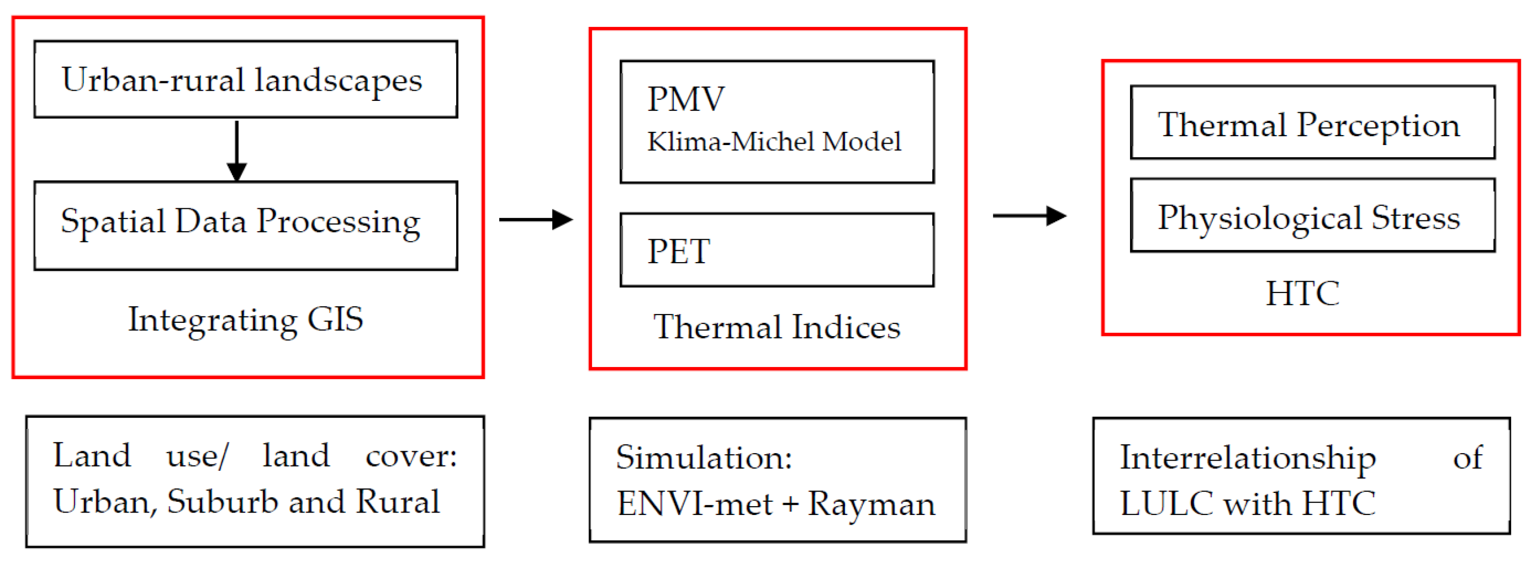
41]), they are not specifically directed at investigating how and to what extent urban-rural gradients and different land use land cover (LULC) types are associated with HTC. More precisely, research examining the relationships of different spatial settings, particularly encompassing a spectrum of urban, suburban, and rural contexts toward HTC is often overlooked, which this study seeks to address. This paper, thus, aims to examine how LULC affects HTC on the basis of the simulation of PMV and PET indices. Furthermore, diurnal variations of air temperatures with different LULC are also assessed. In this case, the PMV index is particularly used for maps’ production because PET maps are not available in the free-version of ENVI-met. To have a better understanding of the paper’s direction and contribution, a conceptual-methodological framework is formulated to highlight the interrelationships between urban-rural landscapes and HTC (see 
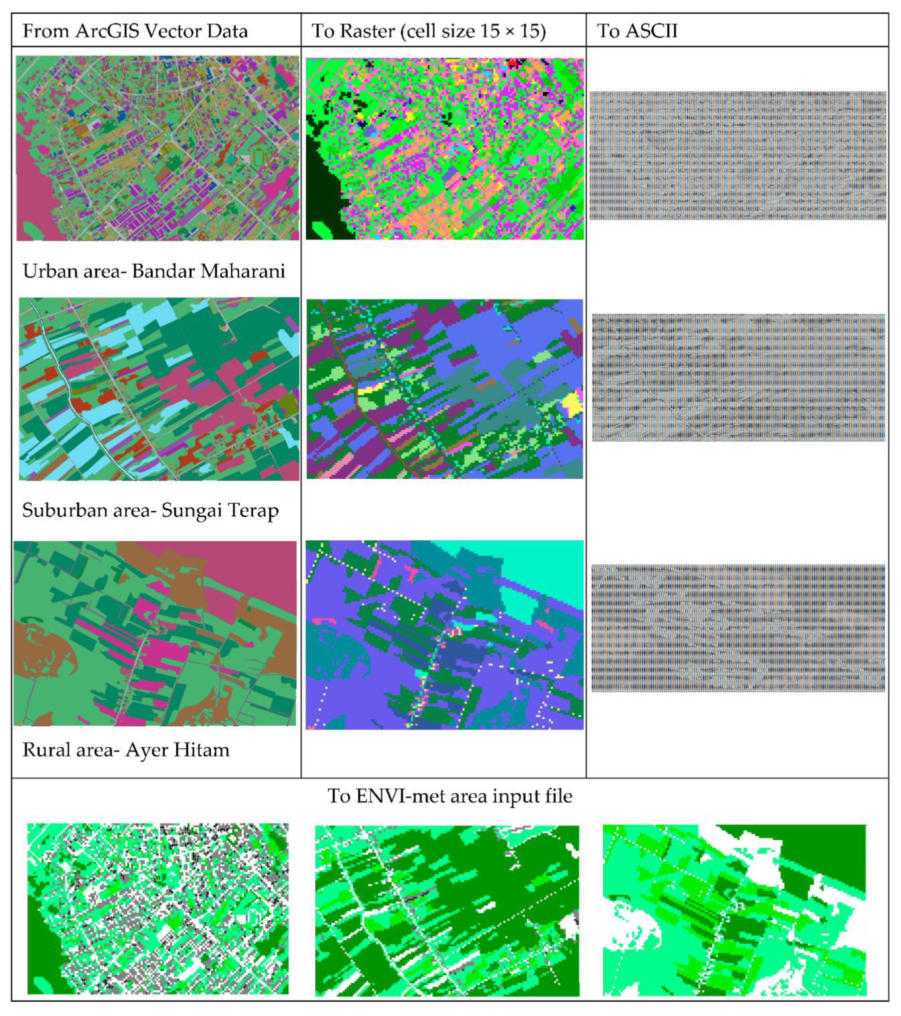
Figure 1). The framework also illustrates how LULC data are processed in the Geographic Information System (GIS) and further integrated with building, vegetation, soil, and surface material models in the ENVI-met model to produce PMV and PET indices, with the aids of the Rayman model (see more in Section 2.2.2, Section 2.2.3, Section 2.2.4 and Section 2.2.5). Consequently, thermal perception and physiological stress can be assessed under different spatial settings. Primarily, there are threefold contributions of the study. First, this paper contributes to the study of HTC in an outdoor context, comparing different urban-rural landscapes in a relatively large mapping scale (with 4.5 km
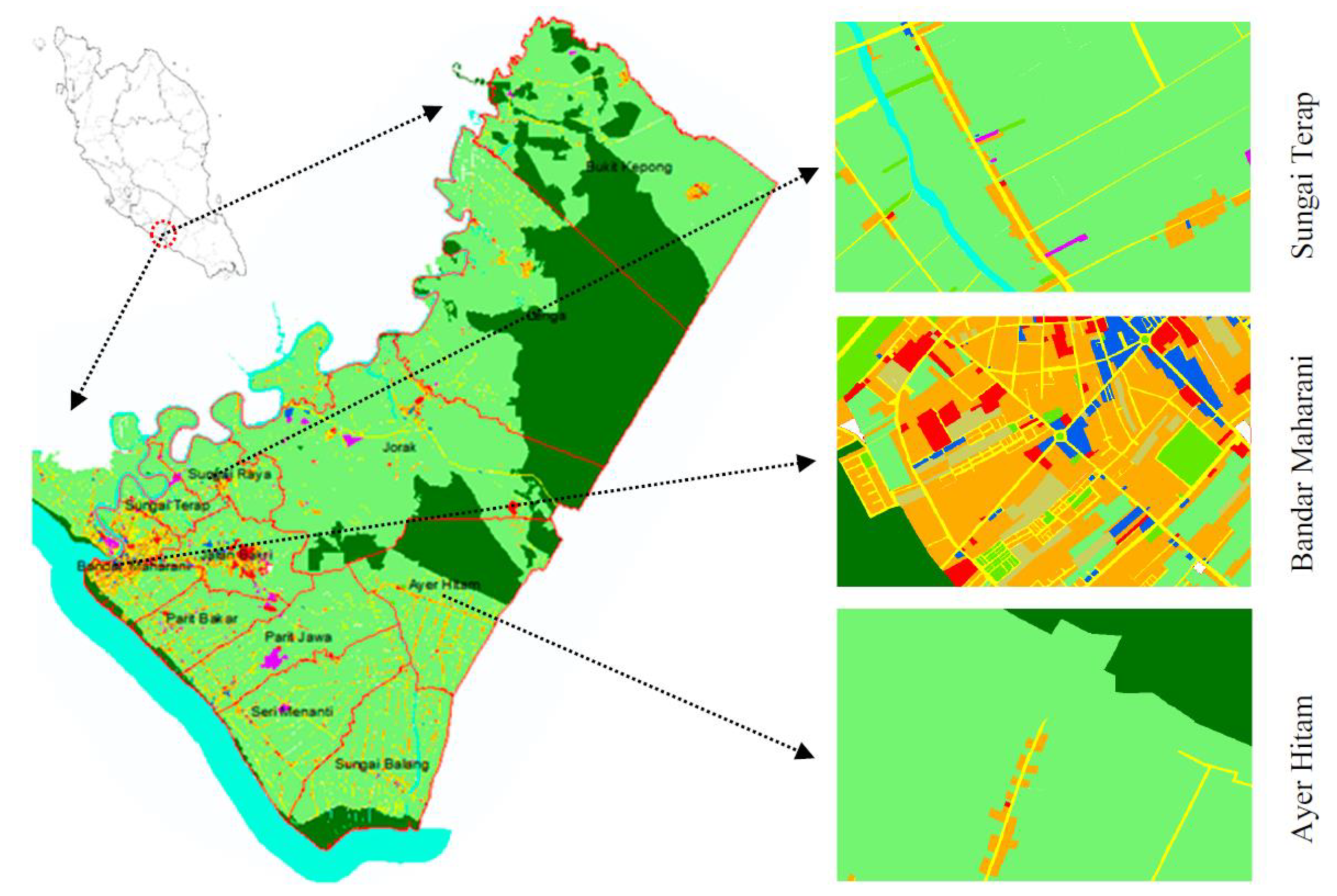
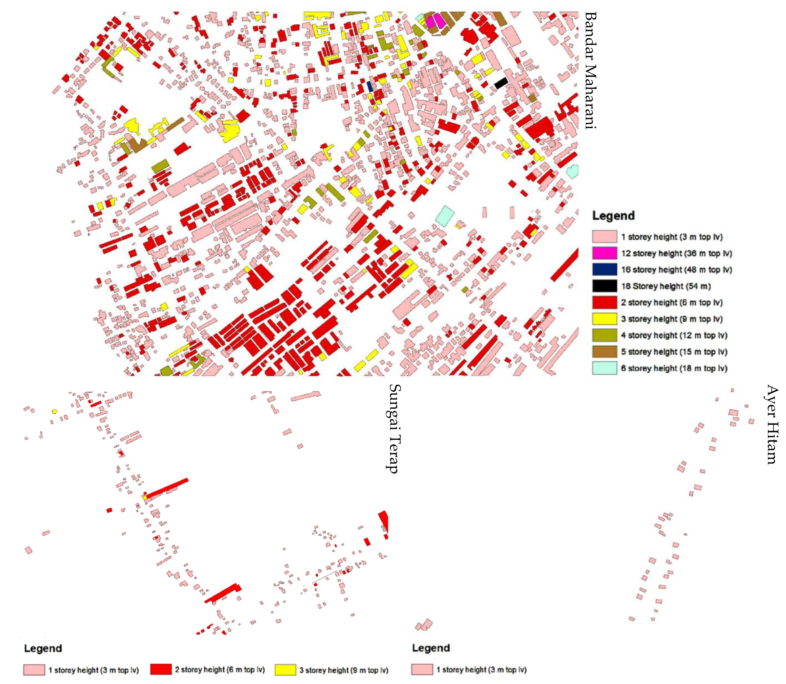
2 and above), despite the general assumption that a large-scale simulation may provide inaccurate results. More specifically, this study becomes an important reference for potential studies that also adopt a rather large-mapping scale of the climatic-HTC approach. Secondly, comparing different LULCs with HTC provides us insights that show which landscape patterns relent heat gains or losses and other climatic factors, subsequently affecting the HTC. Lastly, in terms of the methodology, the integration of LULC data in GIS with ENVI-met also brings a new cognizance in the field of the microclimate simulation, where it makes large-scale simulation more feasible.

2. Materials and Methods

2.1. Study Area

The study area was in the Muar district of Peninsular Malaysia. Maximum, mean, and minimum temperatures in Malaysia range from 29.79 to 33.50 °C, 25.76 to 28.28 °C, and 22.75 to 25.15 °C, respectively [42]. Three areas were plotted, as shown in Figure 2. The dimension of the plots is 2.7 km × 1.8 km. The plotted areas were selected on the basis of the compactness of built-up areas and LULC (see Yeo et al. [43]). The spatial data provided by the Department of Agriculture Muar did not have the attributed information, such as tree height, building height, and surface materials, that are required to run the ENVI-met simulation. Therefore, a field survey was conducted to update the LULC map and collect all the tree height, building height, and surface material information for ENVI-met simulation. The surface materials were identified on-site; tree height was calculated using the basic trigonometry-tangent method (see Larsen et al. [44]), and building height was calculated by the number of floors—one floor is equivalent to a three-meter height.
In the Muar district, plant specifies are diversified. One of the constraints was to collect information (e.g., leaf area index, clear trunk height, and canopy structure) on various trees. For this reason, instead of using the local plant species to create a new database, we adopted the existing ENVI-met plant database. Hence, we only identified the most found species in Muar (see Table 1) and coded them into the ENVI-met plant database accordingly.

2.2. ENVI-Met 4 as a Microclimate Simulation Model

The creation of a microclimate simulation model (ENVI-met) has allowed researchers and practitioners around the world to simulate and study the surface–plant–air interactions [46]. In fact, Ali-Toudert and Mayer [47] posit that ENVI-met is suitable for analyzing thermal comfort because it considers various climatic factors, including air and surface temperatures, wind speed and direction, air humidity, short-wave, and long-wave radiation fluxes, and mean radiant temperature. Evidence suggests that the results simulated using ENVI-met are commendable, i.e., many scholars posit that the simulated results have shown some good agreement with empirical site measurement (see Spangenberg et al. [48]; Peng & Jim, [49]; Berkovic et al. [37]).

2.2.1. Input Parameters

Model input parameters are required to perform a simulation through ENVI-met, for example, area input file, configuration file, and database [50]. Besides, it is important to know certain assumptions in ENVI-met. For instance, the assumptions in the ENVI-met simulation are that: (i) the terrain is always flat; (ii) the shape of the building is in box-shape; (iii) initial meteorological settings need to be set as trial and error until getting a good linkage with measurement data; (iv) there is a constant wind profile; (v) buildings have a constant temperature where anthropogenic heat is not calculated; and (vi) there is a need to configure the tree details such as height and LAI, otherwise the existing database can be used as a representation (Berkovic et al. [37], p. 1175). Under this assumption, it is important to test or validate the simulated results with on-site measurement or data from the meteorological department.

2.2.2. Area Input File

For the area input file, we derived the spatial data from ArcGIS and converted them to the ASCII format, using a conversion tool in GIS, i.e., Raster to ASCII. ASCII is a text file representing raster data. The ASCII data are longer because of the conversion of digits from a single unit to binary units to ease the coding process afterwards. Next, all the ASCII codes were re-processed in WordPad, following the standard unit of binary codes in the ENVI-met database (see the maps in Figure 3). During the re-coding process, the search and replace tool in WordPad was used. All the existing codes were replaced with building, vegetation, soil, and surface material model codes in ENVI-met. For instance, a building using numbers like 03 is equivalent to a 3 m height building, while 15 means a 15 m height building. The vegetation model has its own code as well, for instance, grass (XX), 15 m height tree (SK), 20 m height tree (SM), 10 m height tree (T1). Similar steps were applied to the soil and surface material models as well. It is important to note that when recoding in WordPad, no data value will appear in number −9999. Therefore, if data were in the form of numbers, they must be treated first, otherwise when importing to ENVI-met, the software may not recognize the numbers. After importing, an area input file was generated by ENVI-met itself, shown in Figure 3. The size of the model was 2.7 km × 1.8 km. The details of the buildings, vegetation, and surface materials are explained from Section 2.2.3, Section 2.2.4 and Section 2.2.5.

2.2.3. The Building Model

The height of the buildings ranged from 3 to 54 m (see Figure 4). At the creating model domain, we selected B (2)-brick walls (burned) for a default wall property, and R (1)-tiles for the roof property for an urban area. Meanwhile, buildings in suburban areas were set to brick walls (burned), since the thermal properties of every single structure is not possible to define individually. On the other hand, there is no timber wall material in the database, hence, we used the same B (2)-brick walls with modified thermal transmittance for rural areas. For the roof properties, we selected IR—iron roof, the value of which was calculated on the basis of the Malaysian standard (MS 2680:2017, p. 46 and 52).
The indoor temperatures, thermal transmittance of the walls and roofs, and the albedo coefficient of the walls and roofs are different for each respective site (see Table 2). The indoor temperature Ta,i was set at 293 K (ISO, 2007) was kept constant during the simulation. The thermal transmittance of the wall Kw was set on the basis of the wall of a typical residential building in Malaysia (Saidur et al. [51]). For the albedo coefficient of the walls, it was set at 0.3 for brick walls and 0.4 for timber walls (Taha et al. [52], p. 23). At the same time, the albedo of the roof was based on the ENVI–met-material database.

2.2.4. The Vegetation Model

For the vegetation model, we only identified the most found species and generalized them by their heights and densities (see Figure 5). For palm trees, such as Elaeis guineensis, Cocos nucifera, and Adonidia merrillii, they were categorized under P1 (tree 10 m dense, leafless base) in the ENVI-met database that we had created, which we modified from the existing database, T1. Meanwhile, trees, such as Pterocarpus indicus, Peltophorum pterocarpum, Durio zibethinus, Samania saman and other forested species, were grouped into one category and coded as SM (tree 20 m very dense, distinct crown layer). Parkia speciosa, Ficus microcarpa, and Hevea brasiliensis were grouped and coded as SK (tree 15 m very dense, distinct crown layer). Mangifera indica and Calophyllum inophyllum were coded as S1 (tree 10 m very dense, distinct crown layer), which we created by modifying from the existing database, SK. The rest of the trees, especially those around 5 m height or below were all classified as S2 (tree 5 m dense, distinct crown layer), modified from T1.

2.2.5. Soil and Surface Material Models

There are two categories of soil profile in our study areas, i.e., loamy soil and sandy soil. For loamy soil, it was coded as LO (loamy soil), while sandy soil was coded as SD (sandy soil). Meanwhile, most of the major roads are asphalt roads, so it was coded as ST (asphalt), while certain areas such as playgrounds, stadiums, or industrial areas are covered with a concrete render, hence they were coded as PL (concrete pavement light). Meanwhile, a few places are covered with natural granite stones, hence they were coded as GR (granite). Natural elements such as a river and lake were coded as WW (water), and groundcovers and shrubs were categorized as XX (grass 50 cm average, dense). The maps of the surface materials are referred to in Figure 6.

2.3. Nesting Grid and Cell Size

Initially, we had attempted the simulation with the cell size of 10 m × 10 m in order to cover the whole study area, alas, the simulation failed, due to the floating error, as the computer was not able to handle the simulation or the software itself because it is not appropriate for this large-scale simulation. One area took approximately 4 to 7 days to complete the simulation and this process constantly faced crashes. For this reason, we opted to increase the cell size to 15 m × 15 m. However, increasing the cell size may lead to inaccurate results, because the smaller the cell size, the closer the simulated results with the real experimental results [50]. Hence, to justify the validity of the constructed model, comparing our simulated results with the data from Meteorological Department Malaysia (MET) is mandatory (see Section 2.7).

2.4. Configuration File

For the configuration file (see Table 3), the basic setting included total simulation time, meteorological settings, and output directory. To avoid problems arising and inaccuracy results during the initialization of ENVI-met, the total simulation time was set to 48 h and only the second day was used to exclude the initial transient condition. The reason for the simulation date set was because, firstly, we just finished upgrading the entire database. Secondly, 23 January 2016 was the day with a clear sky condition—little to no clouds, on the basis of our observation for a consecutive week from 17 January 2016 to 23 January 2016. The basic meteorological data were acquired from the Malaysian Meteorological Department [53]. The data included wind speed, wind direction, initial atmosphere temperature, specific humidity, and relative humidity. These input data were as shown below.
  • The wind speed data from MET was in the km/h unit, therefore, to convert it to m/s, it was multiplied by 1000 (km to m) and divided by 3600 (h to s). The wind speed data acquired from MET was 9 km/h (average) and changed to 2.5 m/s after the conversion. The wind direction was north east, and when changing to degree, it was equivalent to 45°.
  • The roughness length (z0) was based on the terrain of the site (see Holmes, [54], pp. 60 on the terrain type and roughness length). The terrain of the Muar district is covered by buildings with a 3 m to 6 m height, mostly. Hence, the z0 value was set to 0.1. Besides, ENVI-met 4 only offers one option on z0 value, and that is 0.1.
  • The air temperature of Muar (potential) was around 30 °C, so converting it to Kelvin (K), it was equal to 303.15. Lastly, the relative humidity was set to 60.3 (average) and the specific humidity was set to 7.8, respectively.
  • The specific humidity at the 2500 m altitude was calculated on the basis of the converter for the humidity of air [55].
All these basic meteorological settings were employed in the microclimate simulation for urban, suburban, and rural areas. It is important to note that, the input data in the configuration file may need to change from time to time until obtaining reliable results (refer to Section 2.7 for the sensitivity result).

2.5. Output File

To calculate HTC, we used the built-in function of ENVI-met 4, namely BioMET v1.01. We did not consider the age group of the people, clothing insulation, and metabolic rate; hence, we applied the default values of clothing insulation (0.9 clo) and metabolism (164.39) in BIOMET, which is based on the standard human ISO 7730. The PMV of the reference person is a 35-year-old male, with a height of 1.75 m and a weight of 75 kg [56] (p. 7). For detailed explanations on how the PMV index was used, the article by Berkovic et al. [37] (pp. 1175–1176) can be referred to, where the authors described the heat exchange between the human body and the thermal environment. Later, we also used the Rayman 1.2 model to calculate the PET value on 24 selected spots and compared it with the PMV values extracted from the ENVI-met simulation.

2.6. Rayman for PET Calculation

Rayman version 1.2 was used to calculate the PET index. We set the date and time in the Rayman model, including the geographic data (Figure 7). The parameters such as air temperature, relative humidity, wind speed, mean radiant temperature, and cloud cover (octas) were extracted from ENVI-met and subsequently keyed into the Rayman 1.2 model. Lastly, personal data, types of clothing, and activities were adjusted on the basis of the standard value of ENVI-met.

2.7. ENVI-Met Model Reliability and Validation Test

The majority of the ENVI-met simulations were validated, known as the sensitivity analysis, through site measurement before finalizing their modelled results. Some research tested on one or two microclimate parameters, such as air temperature (e.g., Ghaffarianhoseini et al. [40]; Peng and Jim, [28]), while other research tested more than two microclimate parameters, such as such as air temperature, surface temperature, relative humidity, global radiation, and solar radiation (e.g., Salata et al. [50]; Liu et al. [57]). In this study, we only tested on air temperature data, since there is a limitation to acquire all the data from the Meteorological Department of Malaysia (MET). To validate the model predictions corresponding to a real situation, most common statistical factors used are the coefficient of determination (R2) accompanied by a test of significance, the Root Mean Square Error (RMSE) and the Willmott’s index of agreement (d) that varies between 0 to 1 for evaluating the goodness-of-fit [58]. There is no absolute recommendation for the values for R2 and d, but as a rule of thumb, the value closer to 1 indicates a perfect agreement, and closer to 0 indicates a weak agreement. Meanwhile for RMSE, the smaller the values the better. Salata et al. [50] has summarized a list of average R2, RMSE, and d values from different studies; the commonly reported result for the validation test usually has an average value of 0.82 (R2), 1.84 (RMSE), and 0.78 (d). Our results are R2 = 0.877 (p-value < 0.005), RMSE = 1.127, and d = 0.916, which are better than the average values reported in the previous study. This means that the simulated results from ENVI-met are considered reliable (see Figure 8). Our result from 9 a.m. to 7 p.m. was quite consistent with the approximate 1 °C variation, while after 10 p.m. to 12 a.m., the gap broadened to a 2 °C variation. These may be due to several factors, but not limited to, e.g., the diurnal variations overestimation or the over-calibration of configuration files in ENVI-met to achieve a good model fitness, and there is a possibility of the large cell sizes affecting the long-wave radiation calculation of the model. Nevertheless, this does not mean that the accuracy of the result would be affected, because the data point used only showed a 0.5 °C variation at 6 p.m.

2.8. Modification of PMV and PET

In this paper, we only displayed the PMV and PET distribution results at 6 p.m. because it was the peak hour, in which people were having their outdoor recreational activities. It is worth to note that the thermal comfort perception for temperate and tropical regions are slightly different. For instance, people who stay in the tropical region are likely to have better heat tolerance than temperate regions (see Makaremi et al. [38]). This study specifically adapted the PET index by Makaremi et al. [38] and Ghaffarianhoseini et al. [40] and modified the PMV index by Honjo [26] to better fit the thermal perception classification of PET (see Table 4).

3. Results & Discussion

The results presented here are separated into three sections to answer how LULC affects HTC. Firstly, Section 3.1 illustrates the overall thermal perceptions between urban, suburban, and rural areas. Next, Section 3.2 explains how different types of LULC affect the change of air temperatures from 12 p.m. to 12 a.m. Lastly, Section 3.3 discourses the thermal perceptions (PMV and PET) of the people and their physiological stress at randomly selected points of different LULC.

3.1. Mapping Thermal Comfort of Urban, Suburban, and Rural Areas

The simulation result, shown in Figure 9, illustrates that 25% of Bandar Maharani’s areas had a PMV value ranging from 3.4 to 3.9. This connotes that people have a propensity to undergo hot thermal sensation and strong physiological heat stress even though it was around 6 p.m. and close to sunset. Those areas included asphalt roads, car park areas, and sandy and loamy soil surfaces that lacked shaded trees and infrastructures. Worse still, 2% of the areas had a PMV value reaching 4.1. On the other hand, 47% of the areas had a PMV around 2.6 to 2.9. Most of these areas were grass-covered and without the existence of trees. While only 8% of the areas were below the PMV of 2.4, those areas happened to be shaded by trees and buildings (e.g., lowland forest, agriculture plantation, and alleys). Nevertheless, people still felt slightly warm and experienced slight heat stress. In this case, we believe PMV values ranging between 1.5 and 2.5 are generally acceptable by most people in Malaysia because those living in a tropical region usually have a better tolerance towards heat [38]. Similarly, Berkovic et al. [37] also posit that the PMV value below 2.0 is considered as a desirable condition.
As opposed to Bandar Maharani, more than half of the areas of Sungai Terap had a PMV value around and/or less than 2.4. Most of these areas were covered with agricultural plantations (e.g., durian trees, rubber trees, and oil palms), and the trees shade most of the surface areas, thus obstructing and storing heat from solar radiation. This situation also promotes evaporative cooling through leaf absorption, transmission, and reflection [14,15]. Similarly, Ayer Hitam’s LULC consisted of many agricultural plantations (62%), and it is partially covered with the lowland secondary forest (13%). Of Ayer Hitam areas, 43% had PMV between 2.1 and 2.4, in which we anticipated that the thermal comfort of suburban and rural areas should be alike. However, the result showed a variation, due to the excessive vacant ground surface, i.e., 10% of the area had PMV around 3.4 and above, which took place at the vacant ground.

3.2. LULC Influencing the Air Temperatures Distribution

The diurnal variation of air temperatures (23 January 2016) showed that the highest air temperatures in the urban, suburb, and rural areas were found at LULC with man-made features. The points of the receptors are shown in Figure 6. For instance, Bandar Maharani (Figure 10) and Ayer Hitam (Figure 11) had the highest air temperatures (33.5 °C and 32.8 °C) at 4 p.m. on asphalt surface. Surprisingly, the concrete surface of Sungai Terap (Figure 12) exhibited a hotter air temperature (33.1 °C) than the asphalt surface (32.9 °C) compared to Bandar Maharani, where the asphalt surface (33.5 °C) had a slightly higher air temperature than the concrete surface (33.3 °C) at 4 p.m.. We suspect that this phenomenon happened due to the total area and coverage of the albedo material. The concrete surface at Bandar Maharani is much smaller than the one at Sungai Terap. Thus, the reflection of short-wave radiation on the concrete surface at Sungai Terap was higher than Bandar Maharani; it contributed to warming up the air mass and consequently resulted in the increase of the air temperature. On the other hand, since the asphalt road is mainly surrounded by agricultural plantation providing evaporative cooling, it could possibly lower the surrounding air temperature. In this case, it is difficult to judge the de facto factors affecting the temperature. Hence, more studies regarding this scenario can be conducted.
From the graphs, illustrated in Figure 10, Figure 11 and Figure 12, we noticed that the area covered by trees had the lowest air temperature, most of the time, whereas the air temperatures near built-up, concrete, and asphalt areas were relatively higher than tree-covered and lawn areas. These findings affirm previous studies [14,15,18,59] that the air temperature of non-natural features, especially on the low-albedo surface (e.g., dark asphalt road), is higher compared to natural features, such as forested areas. Meanwhile, sandy and loamy surfaces tend to emit more heat during nighttime. One of the factors was that they absorbed heat slowly during daytime, and thus the heat was retained much longer. As a result, the long-wave radiation was slowly released during nighttime. The size of the LULC also influenced the heat absorption; the loamy surface at the rural area which is wider than suburb area accumulated higher heat. Indeed, the study area, Muar, is faced with the urban heat island effect, where our simulated results have demonstrated that temperatures of LULC at urban areas were warmer than suburban and rural areas by 1 to 2 °C during night time.

3.3. LULC and Human Thermal Comfort

The simulation results extracted from ENVI-met 4 and calculated by Rayman 1.2 are presented in Table 5, Table 6 and Table 7, respectively. The points of the receptors are shown in Figure 9. The vapor pressure was automatically calculated by Rayman, after keying in the information of the air temperature and humidity. The dense canopy forested area, with an average of 20 meters’ height, FR (1), at Bandar Maharani had the lowest PMV and PET (see Table 5), compared to other spatial settings. This suggests that people were inclined to experience slight heat stress and feel slightly warm, but it is still under an acceptable thermal preference. We anticipated that during cloudy days, the comfort level would be much better because the solar radiation is more intense under the clear sky condition (see Emmanuel et al. [60]). Within a forested area with the average 15 m height, FR (2), the PMV and PET were slightly higher than FR (1), due to the low wind speed and the high mean radiant temperature (Tmrt). The wind speed was particularly low in FR (2) because the surrounding buildings obstructed its speed and altered the direction. Meanwhile, the Tmrt of FR (2) was slightly higher because the tree height and density were different from FR (1). This also has been reported by Spangenberg et al. [48] that a high-density canopy performs better than a low-density canopy in mitigating the Tmrt value.
For the grass-covered areas (Table 5), GS (1) and GS (2), people were feeling warm and experiencing moderate heat stress. Albeit both areas were classified as the same thermal perception and physiological stress, GS (2) performed slightly better than GS (1). One of the contributing factors is the size. The size of grass-covered areas at GS (1) is almost twice the size of GS (2). A huge patch of grass-covered areas have the higher propensity to convert some of the solar energy into sensible heat on the basis of the Penman–Monteith equation, where many small patches of grass areas are more effective in providing the cooling effect through evapotranspiration, due to the oasis effect (see Armson et al. [18]). Besides, the wind speed of GS (2) was slightly better than GS (1), which also may improve the human thermal comfort through convection. As a result, the HTC of GS (2) is better than GS (1).
For the asphalt road—AP (1) and car park—AP (2), both sites were categorized in the same thermal classification, in which people felt hot and experienced strong heat stress. This is because both points AP (1) and AP (2) were directly exposed to the direct solar radiation (without shading), and the asphalt surface was heated up much more than the greenery, due to its albedo properties. Similar case also happened to LO (1) and SA (1), where the surface temperatures of AP (1), AP (2), LO (1), and SA (1) were also likely to escalate the long-wave radiation from urban surfaces and contribute to the increase of Tmrt. This suggests that the increase of Tmrt has shown a relationship with human thermal comfort. Our results presented here shows a positive correlation between Tmrt and PMV or PET. When Tmrt decreases, PMV and PET also decrease and vice versa. These findings are in line with the assertion of Thorsson et al. [33] and Berkovic et al. [37], in which the thermal perception is correlated with Tmrt. From the readings of Tmrt (Table 5), it suggests that the use of high albedo for outdoor LULC seems to be more appropriate, due to the inference of PMV and PET. However, this is not always the case, because of the time factor. Our measurement was based on 6 p.m., during which the reflection of solar radiation was not that intense. Thus, the absorption of solar radiation by low albedo materials, such as AP, LO, and SA increased the long-wave radiation, and that was the main factor contributing to thermal distress. In reality, people are more active during daytime; thus, it is not encouraged to use high albedo materials for paths or routes, due to the high reflection rate of solar radiation. Meanwhile, to promote synergies between creating a comfort environment and mitigating the UHI effect, the use of high albedo materials for roof top areas are much desired [61].
Similarly, dense canopy agricultural plantations (20 m height)—FR (1) and FR (2) at Sungai Terap had the lowest PMV and PET values (see Table 6). The PMV and PET values at different spatial settings of Sungai Terap were lower than Bandar Maharani. For instance, Bandar Maharani has more urban structures (44.08%), while Sungai Terap has more canopy trees (78.41%). Practically, this will affect the surface radiation and energy balances; trees can act as the medium for blocking-off the direct short-wave radiation from the sun, reducing sky-view factors, and promoting evapotranspiration.
Both FR (1) and FR (2) had PMV and PET values, classified as a slightly warm thermal perception, where people experienced slight heat stress. Nevertheless, the PMV and PET values of the dense canopy area FR (1) near the waterbody of Sungai Terap had better PMV and PET values compared to FR (2). This is because FR (1) was synergized well with the river, thereby improving the cooling effect of the waterbody on HTC. This also has been affirmed by Xu et al. [62] that the human comfort level in an vegetated area at a littoral zone may perform more effectively than non-vegetated areas. However, it was also pointed out by Theeuwes et al. [63] and Xu et al. [64] that a waterbody could hamper the heat balance and sensations of the human body and could cause sensory discomfort through the increase of humidity. In our context, we believe that the illation of humidity is not that significant, compared to wind velocity and Tmrt. Meanwhile, it is worth noting that the cooling effect of the waterbody is only effective during daytime, when the night warming effect is triggered [63]. Hence, it is important to consider the advantages and disadvantages when proposing a waterbody in designing and planning for our everyday landscapes because it does not always entail that the more waterbodies are provided, the better they contribute towards human thermal comfort. Next, AP (1) and CO (1) were considered as the hottest areas in which people tended to feel hot and experience strong heat stress. The PMV and PET values of CO (1) were lower than AP (1), which was not surprising at all due to the strong wind promoting heat to leave the bodies through convection. Consequently, the thermal comfort perception of the people at CO (1) was slightly better than AP (1).
As for Ayer Hitam, relatively similar to Sungai Terap, the PMV and PET values of different spatial settings were slightly better than Bandar Maharani. The lowest PMV and PET values (see Table 7) still occurred at a dense canopy forested area—FR (1) and a dense canopy agricultural plantation—FR (2). The highest PMV and PET values, due to asphalt roads AP (1), exhibited the same results as Bandar Maharani and Sungai Terap. In this section, we highlighted three different grass-covered areas—GS (1), GS (2), and GS (3), respectively (see Figure 8, Ayer Hitam’s map), with different contextual settings. For instance, GS (1) was surrounded by barren ground, GS (2) was surrounded by an agricultural plantation, and GS (3) was surrounded by wild grasses. Our results demonstrated that the variation is not apparently significant, however, the value of PET showed some small changes. That is, GS (3) was slightly better than GS (1) and GS (2), due to the low air temperature and Tmrt. This was probably due to the air humidity and the wind speed. Even though GS (1) was a windy area, due to its openness, the air temperature was considerably high, due to the influence of the surrounding barren ground. Meanwhile, the air temperature at the location of GS (3) was lower than GS (2), due to the existence of adjacent trees. The adjacent trees also restricted the wind speed and direction, hence affecting the wind flow to ventilate the heat. Therefore, for the spatial design for the purpose of improving the thermal comfort of the people, it is pivotal to consider multiple perspectives, including the location, tree species (canopy), surface material (albedo), sky-view factor, and wind direction and speed for better coordinated decision making, especially in the microclimate regulation.

4. Conclusions and Recommendations

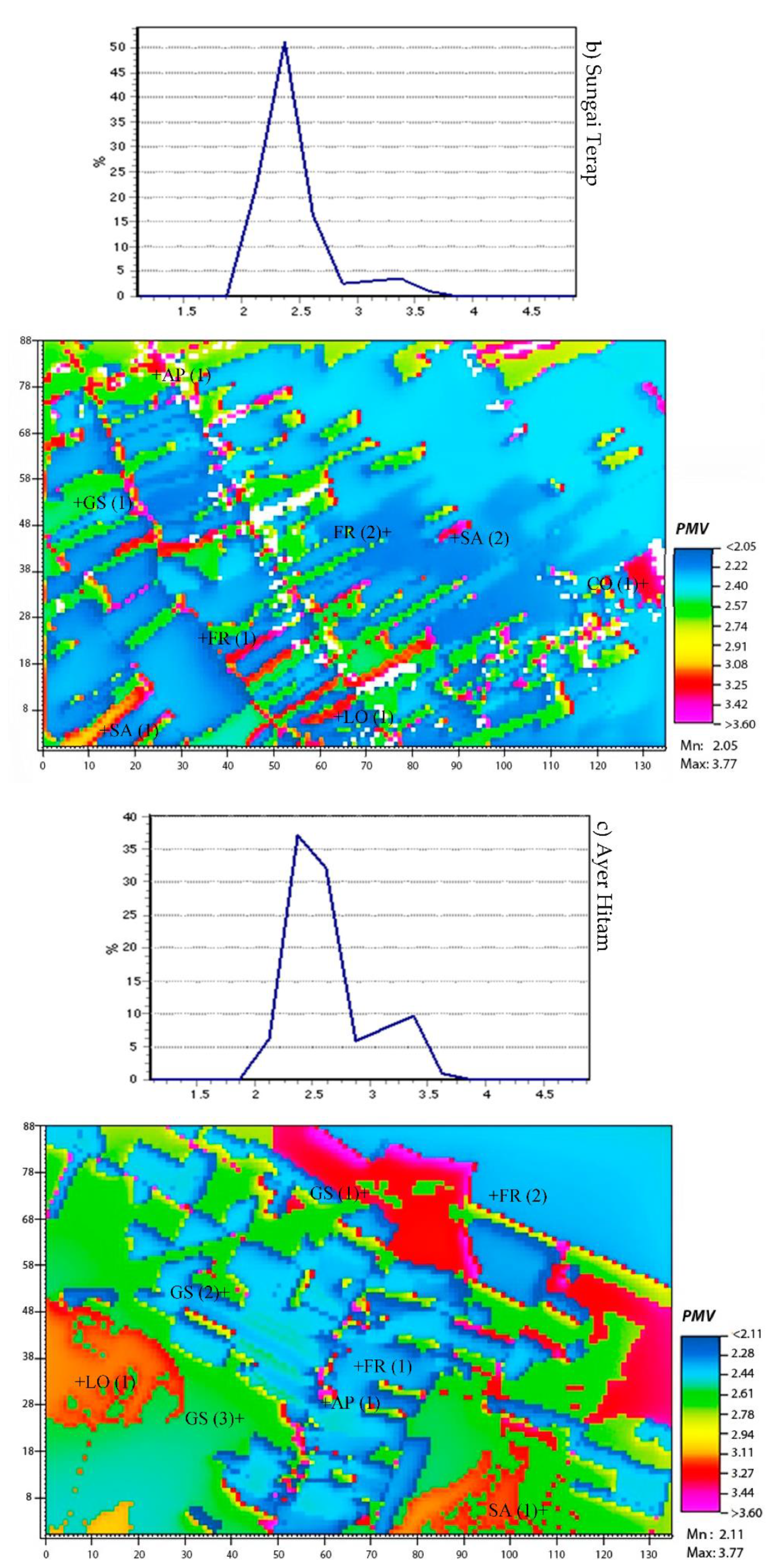
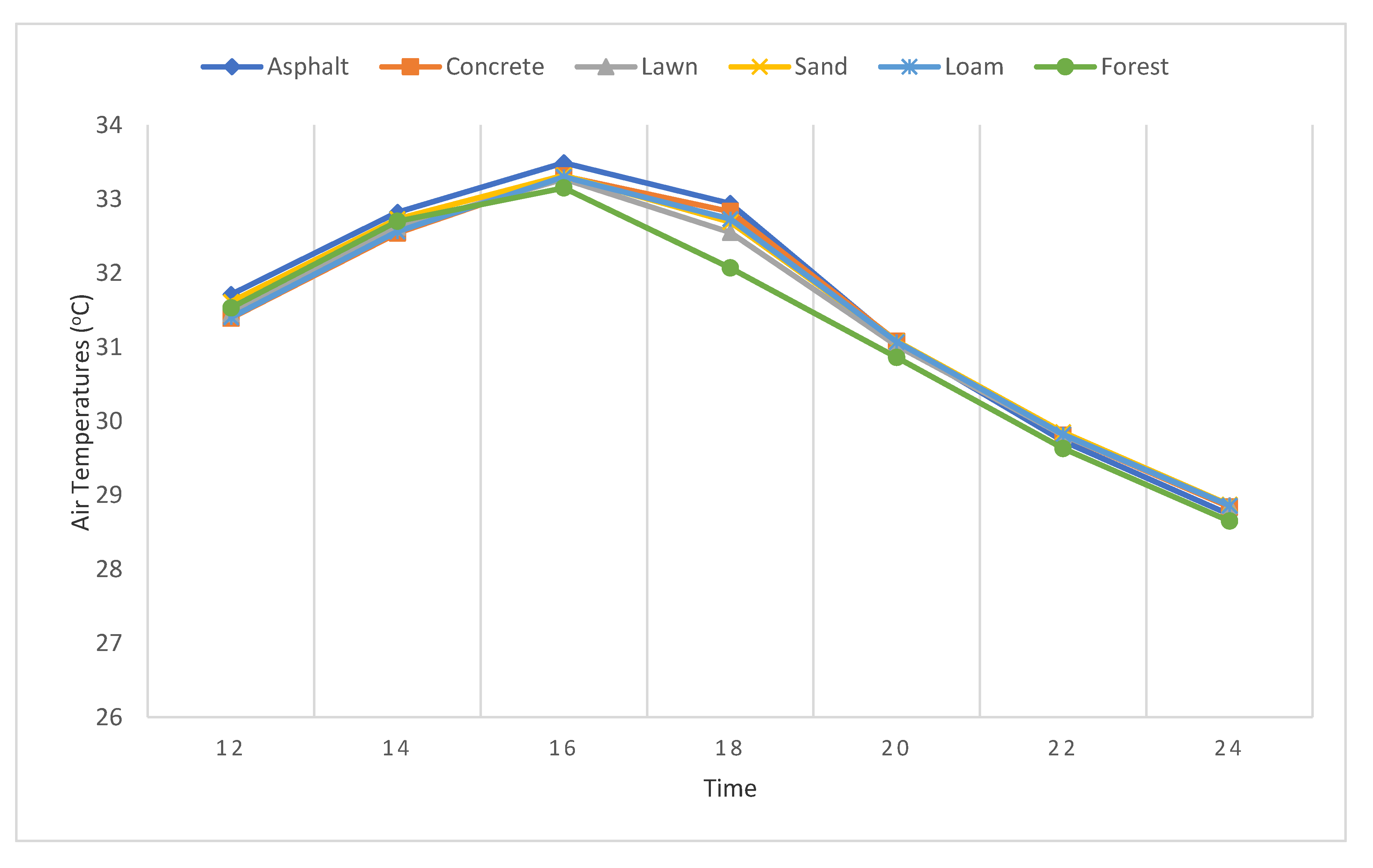
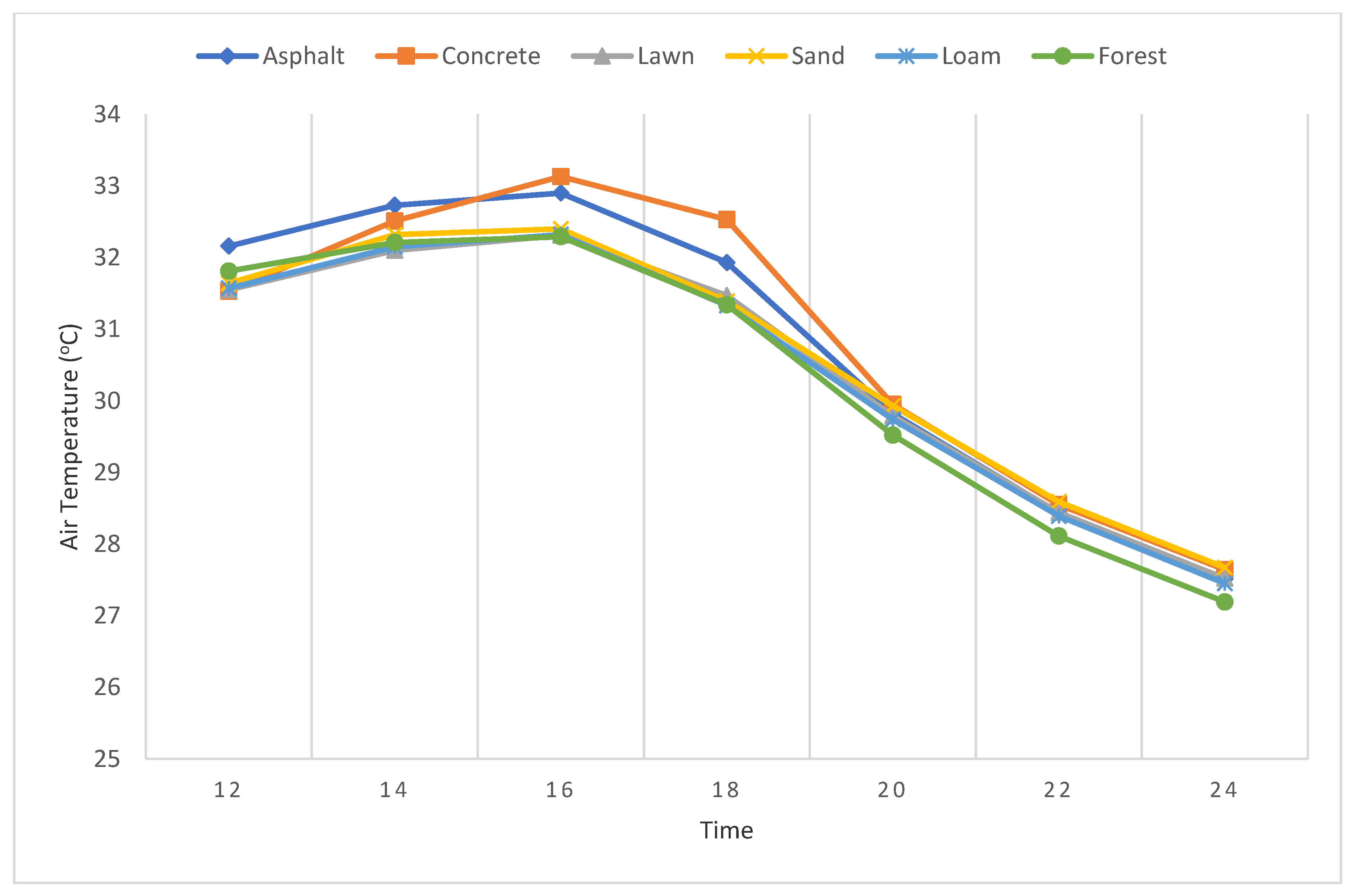
HTC is an essential element in the built environment; improving HTC is challenging, considering its various aspects/determinants (e.g., air temperature, humidity, wind speed). Although numerous studies have been conducted to investigate how physical planning factors (i.e., LULC) influence UHI, very few were focused on a spectrum of urban-suburb-rural effects on HTC. Considering the large number of man-made features in urban areas, a general assumption is that urban areas are always warmer than suburbs, and suburban areas are warmer than rural areas. Our findings on the air temperature distribution agree with this statement; the air temperature for various LULC in urban areas is 1 to 2 °C hotter than suburban and rural areas. However, the influence of LULC towards HTC shows a different trend, in which the key findings are summarized as follows:
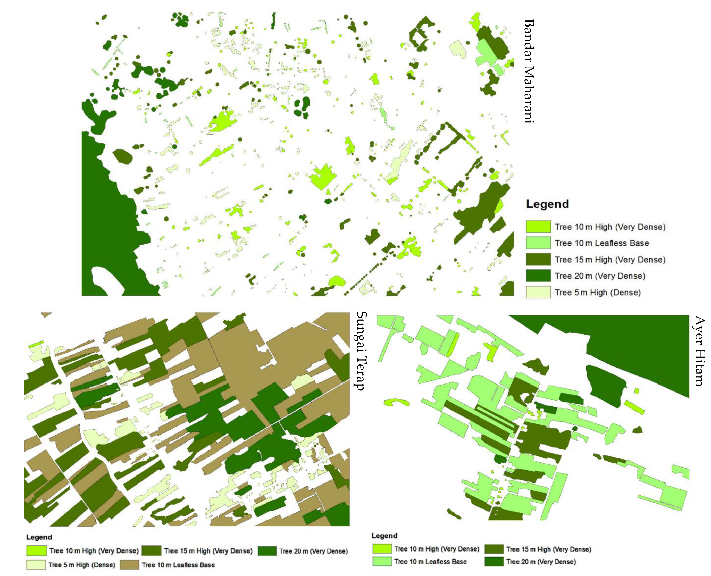
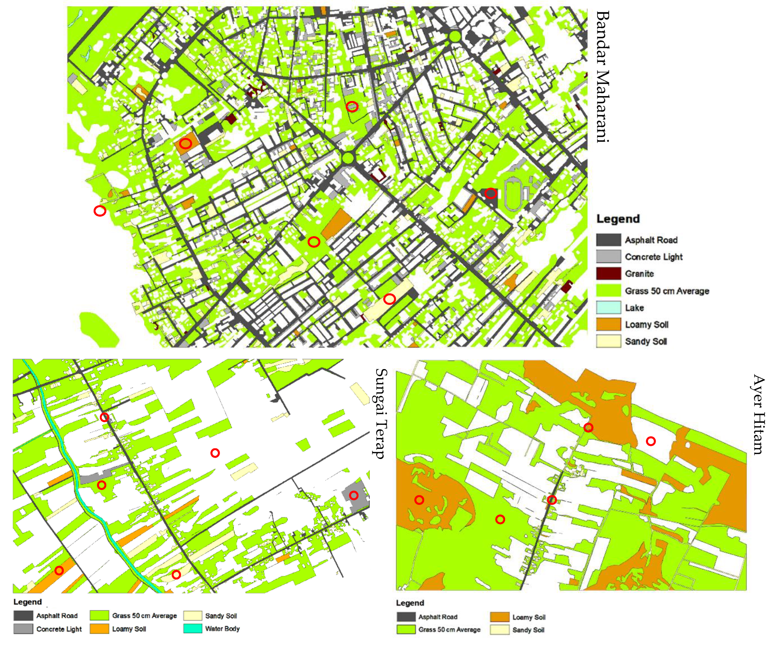
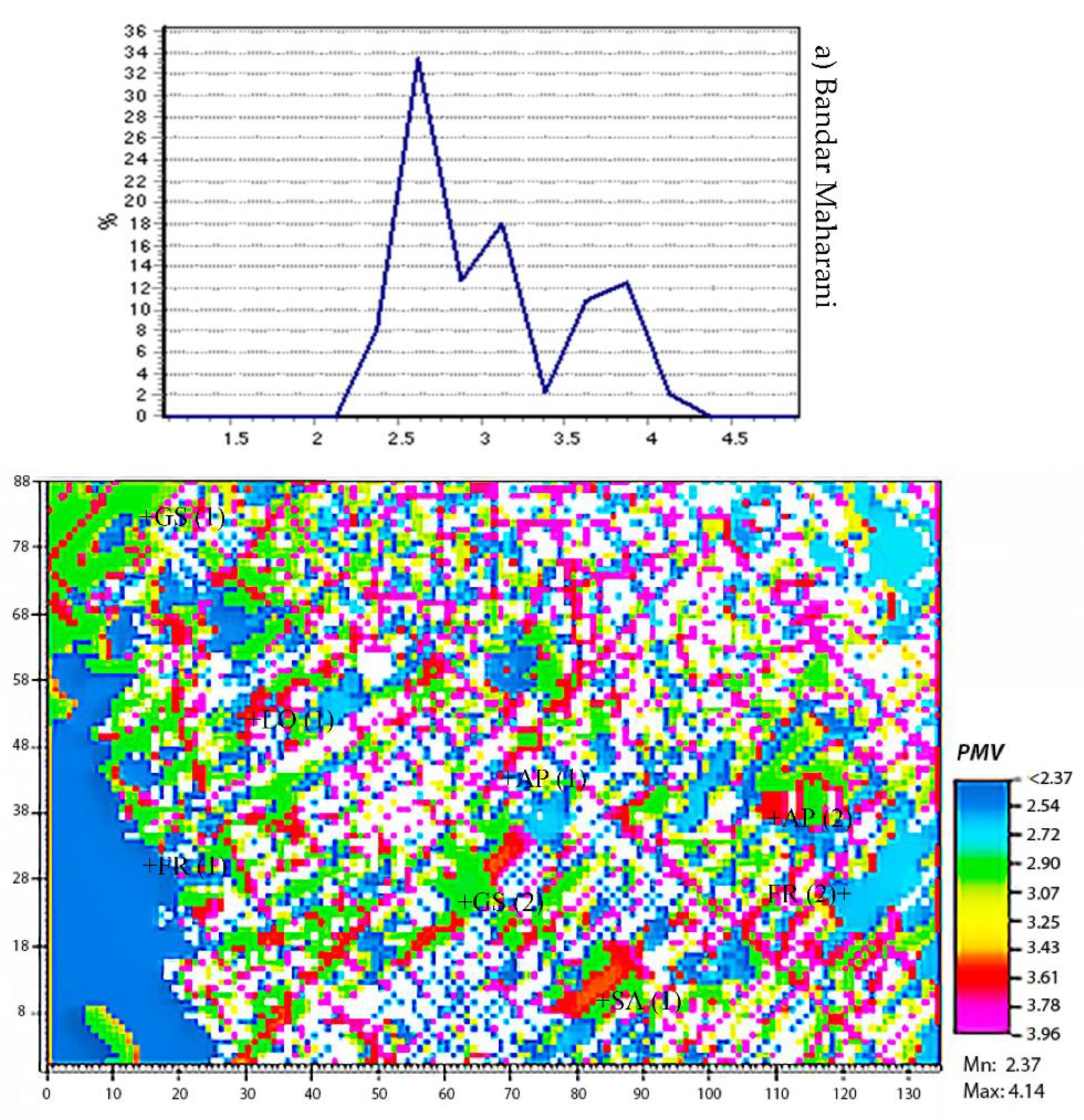
First, it is demonstrated that people living in an urban area have a higher chance to experience strong heat stress and hot thermal sensation, where 25% of the areas have PMV ranging from 3.4 to 3.9, and 2% of the areas have PMV reaching as high as 4.1, followed by 43% of the rural areas with PMV ranging from 2.1 to 2.4, and lastly the suburban area (more than 50% of the areas with PMV values less than 2.4). This shows that people in rural areas are at times susceptible to experiencing heat stress and hot thermal sensation. The reason is that people living in the rural area, in our case, tend to experience higher heat stress, due to the excessive heat generated from deforested barren land. Hence, the general assumption that rural areas have better HTC may not always be true, due to lower air temperature distribution. Second, our findings also show that tree-covered areas have the lower thermal index with PMV ranging from 2.1 to 2.4 and PET from 30.7 to 34.4, compared to open areas, such as asphalt streets, car parks, concrete areas, and sandy and loamy areas—vacant land with PMV ranging from 2.9 to 3.7 and PET ranging from 33.8 to 41.5. Meanwhile, tree-covered areas near the river in the suburban area afforded the best thermal experience with PMV of 2.1 and PET of 30.7, due to evaporative cooling and shading effects. This signifies that the synergy between the water element and greenery is crucial to create a more comfortable environment. This further suggests that future urban and city development can consider including these two factors into planning and design consideration. More precisely, in the context of Malaysia’s strategic spatial planning system, LULC-HTC considerations covering the following factors, namely tree species (canopy density), surface material (albedo), sky-view factor, and wind direction and speed are vital to be included in better devising statutory local plans (a land use/zoning plan) and landscape plans. In sum, tree-covered areas offer the best thermal experiences followed by grass-covered areas. Meanwhile, man-made features, such as asphalt streets and concrete surfaces and vacant ground, be it sandy and loamy surfaces, offer the worst thermal experiences to its users.
Despite the above contributions, this study is subject to some limitations; future research can take them into consideration, particularly when doing a large-scale simulation. First, this is one of the largest simulation maps presented to-date, hence time and hardware factors restricted our simulation time to produce a more accurate result. Nevertheless, we statistically proved the reliability of the results through the goodness-of-fit test by comparing the coefficient correlation (R2), standard deviation errors (RMSE), and the agreement index (d), in which all of them obtained optimal levels. Secondly, we only focused on a specific timeframe to analyze how spatial variations in terms of urban-suburban-rural settings influence the thermal comfort of the people. Hence, we suggest future research can consider studying different timeframes, e.g., morning, afternoon, evening, and midnight via a time-series approach. Besides, investigations towards suburban and rural areas are highly encouraged because these areas are normally being neglected in the study of thermal comfort, especially our findings have proven the significant role of dense canopy-covered areas in suburban and rural areas in regulating the thermal comfort of people.
Since the microclimate simulation model has differentiated how various spatial settings influence the thermal comfort of the people, this study helps stakeholders to identify potential hotspots that can be treated. Besides, maps generated through the microclimate simulation model also provide us with insights into which spatial settings and their surrounding offer the best or worse thermal experiences, subsequently treatments can be incorporated to reduce the heat intensity of these areas. Last but not least, these findings are of practical significance, as they can be a guide to practitioners and policymakers, such as landscape architects, urban planners and designers, and environmental engineers in improving the human thermal experiences and subsequently promoting a more livable and sustainable environment.

Author Contributions

Conceptualization, L.B.Y.; methodology, L.B.Y.; software, L.B.Y.; formal analysis, L.B.Y.; data curation, L.B.Y.; writing—original draft preparation, L.B.Y.; writing—review and editing, G.H.T.L., M.L.T., and P.C.L.; project administration, M.L.T.; funding acquisition, M.L.T. All authors have read and agreed to the published version of the manuscript.

Funding

This research was funded by Ministry of Higher Education Malaysia under the Fundamental Research Grant Scheme (FRGS) grant number 203.PHUMANITI.6711695 and the NEWTON-NERC (IMPRESS-Malaysia), grant number 203.PHUMANITI.6780001.

Informed Consent Statement

Informed consent was obtained from all subjects involved in the study.

Conflicts of Interest

The authors declare no conflict of interest.

References

  1. Shrestha, M.K.; York, A.M.; Boone, C.G.; Zhang, S. Land fragmentation due to rapid urbanization in the Phoenix Metropolitan Area: Analyzing the spatiotemporal patterns and drivers. Appl. Geogr. 2012, 32, 522–531. [Google Scholar] [CrossRef]
  2. While, A.; Whitehead, M. Cities, Urbanisation and Climate Change. Urban Stud. 2013, 50, 1325–1331. [Google Scholar] [CrossRef]
  3. Tan, J.; Zheng, Y.; Song, G.; Kalkstein, L.S.; Kalkstein, A.J.; Tang, X. Heat wave impacts on mortality in Shanghai, 1998 and 2003. Int. J. Biometeorol. 2007, 51, 193–200. [Google Scholar] [CrossRef] [PubMed]
  4. Bowler, D.E.; Buyung-Ali, L.; Knight, T.M.; Pullin, A.S. Urban greening to cool towns and cities: A systematic review of the empirical evidence. Landsc. Urban Plan. 2010, 97, 147–155. [Google Scholar] [CrossRef]
  5. Oke, T.R. Street design and urban canopy layer climate. Energy Build. 1988, 11, 103–113. [Google Scholar] [CrossRef]
  6. Rizwan, A.M.; Dennis, L.Y.C.; Liu, C. A review on the generation, determination and mitigation of Urban Heat Island. J. Environ. Sci. 2008, 20, 120–128. [Google Scholar] [CrossRef]
  7. Millennium Ecosystem Assessment. Ecosystems and Human Well-Being: Biodiversity Synthesis; World Resources Institute: Washington, DC, USA, 2005. [Google Scholar]
  8. Oliveira, S.; Andrade, H.; Vaz, T. The cooling effect of green spaces as a contribution to the mitigation of urban heat: A case study in Lisbon. Build. Environ. 2011, 46, 2186–2194. [Google Scholar] [CrossRef]
  9. Susca, T.; Gaffin, S.R.; Dell’Osso, G.R. Positive effects of vegetation: Urban heat island and green roofs. Environ. Pollut. 2011, 159, 2119–2126. [Google Scholar] [CrossRef]
  10. Shishegar, N. The Impacts of Green Areas on Mitigating Urban Heat Island Effect: A Review. Int. J. Environ. Sustain. 2014, 9, 119–130. [Google Scholar] [CrossRef]
  11. Kong, F.; Yin, H.; James, P.; Hutyra, L.R.; He, H.S. Effects of spatial pattern of greenspace on urban cooling in a large metropolitan area of eastern China. Landsc. Urban Plan. 2014, 128, 35–47. [Google Scholar] [CrossRef]
  12. Lindén, J.; Simon, H.; Fonti, P.; Esper, J.; Bruse, M. Observed and modeled transpiration cooling from urban trees in Mainz, Germany. In Proceedings of the ICUC9-9th International Conference on Urban Climate Jointly with 12th Symposium on the Urban Environment, Toulouse, France, 28 May 2015. [Google Scholar]
  13. Zupancic, T.; Westmacott, C.; Foundation, D.S.; Bulthuis, M. The Impact of Green Space on Heat and Air Pollution in Urban Communities: A Meta-narrative Systematic Review; David Suzuki Foundation: Vancouver, BC, Canada, 2015. [Google Scholar]
  14. Taha, H. Urban climates and heat islands: Albedo, evapotranspiration, and anthropogenic heat. Energy Build. 1997, 25, 99–103. [Google Scholar] [CrossRef] [Green Version]
  15. Shahidan, M.F.; Shariff, M.K.M.; Jones, P.; Salleh, E.; Abdullah, A.M. A comparison of Mesua ferrea L. and Hura crepitans L. for shade creation and radiation modification in improving thermal comfort. Landsc. Urban Plan. 2010, 97, 168–181. [Google Scholar] [CrossRef]
  16. Bonan, G.B. The microclimates of a suburban Colorado (USA) landscape and implications for planning and design. Landsc. Urban Plan. 2000, 49, 97–114. [Google Scholar] [CrossRef]
  17. Zhou, W.; Huang, G.; Cadenasso, M.L. Does spatial configuration matter? Understanding the effects of land cover pattern on land surface temperature in urban landscapes. Landsc. Urban Plan. 2011, 102, 54–63. [Google Scholar] [CrossRef]
  18. Armson, D.; Stringer, P.; Ennos, A.R. The effect of tree shade and grass on surface and globe temperatures in an urban area. Urban For. Urban Green. 2012, 11, 245–255. [Google Scholar] [CrossRef]
  19. Aflaki, A.; Mirnezhad, M.; Ghaffarianhoseini, A.; Ghaffarianhoseini, A.; Omrany, H.; Wang, Z.-H.; Akbari, H. Urban heat island mitigation strategies: A state-of-the-art review on Kuala Lumpur, Singapore and Hong Kong. Cities 2017, 62, 131–145. [Google Scholar] [CrossRef] [Green Version]
  20. Wong, N.H.; Cheong, K.W.D.; Yan, H.; Soh, J.; Ong, C.; Sia, A. The effects of rooftop garden on energy consumption of a commercial building in Singapore. Energy Build. 2003, 35, 353–364. [Google Scholar] [CrossRef]
  21. Höppe, P. Different aspects of assessing indoor and outdoor thermal comfort. Energy Build. 2002, 34, 661–665. [Google Scholar] [CrossRef]
  22. Andreou, E. Thermal comfort in outdoor spaces and urban canyon microclimate. Renew. Energy 2013, 55, 182–188. [Google Scholar] [CrossRef]
  23. Fanger, P.O. Calculation of thermal comfort, Introduction of a basic comfort equation. ASHRAE Trans. 1967, 7, 3–4. [Google Scholar]
  24. Fanger, P.O. Thermal Comfort. Analysis and Application in Environment Engineering; McGraw Hill: New York, NY, USA, 1972. [Google Scholar]
  25. Mayer, H.; Höppe, P. Thermal comfort of man in different urban environments. Theor. Appl. Climatol. 1987, 38, 43–49. [Google Scholar] [CrossRef]
  26. Honjo, T. Thermal Comfort in Outdoor Environment. Glob. Environ. Res. 2009, 13, 43–47. [Google Scholar]
  27. Thorsson, S.; Lindqvist, M.; Lindqvist, S. Thermal bioclimatic conditions and patterns of behaviour in an urban park in Göteborg, Sweden. Int. J. Biometeorol. 2004, 48, 149–156. [Google Scholar] [CrossRef] [PubMed]
  28. Peng, L.; Jim, C.Y. Green-roof effects on neighborhood microclimate and human thermal sensation. Energies 2013, 6, 598–618. [Google Scholar] [CrossRef] [Green Version]
  29. Jendritzky, G.; Nübler, W. A model analysing the urban thermal environment in physiologically significant terms. Arch. Meteorol. Geophys. Bioclimatol. Ser. B 1981, 29, 313–326. [Google Scholar] [CrossRef]
  30. Thani, S.K.S.O.; Mohamad, N.; Jamaludin, S. Outdoor Thermal Comfort: The Effects of Urban Landscape Morphology on Microclimatic Conditions in a Hot-Humid City. WIT Trans. Ecol. Environ. 2013, 179, 651–662. [Google Scholar]
  31. Srivanit, M.; Auttarat, S. The Summer Thermal Environment and Human Comfort of Shaded Outdoor and Semi-Outdoor Spaces to Living in the Urban Area of Chiang Mai City. J. Archit. Plan. Res. Stud. (JARS) 2015, 12, 53–72. [Google Scholar] [CrossRef]
  32. Lucchese, J.; Andreasi, W. Designing Thermally Pleasant Open Areas: The Influence of Microclimatic Conditions on Comfort and Adaptation in Midwest Brazil. J. Sustain. Dev. 2017, 10, 11. [Google Scholar] [CrossRef] [Green Version]
  33. Thorsson, S.; Lindberg, F.; Eliasson, I.; Holmer, B. Different methods for estimating the mean radiant temperature in an outdoor urban setting. Int. J. Climatol. 2007, 27, 1983–1993. [Google Scholar] [CrossRef]
  34. Huttner, S.; Bruse, M.; Dostal, P. Using ENVI-met to simulate the impact of global warming on the mi- croclimate in central European cities. In Proceedings of the 5th Japanese-German Meeting on Urban Climatology, Freiburg, Germany, 6 October 2008. [Google Scholar]
  35. Chen, L.; Ng, E. Outdoor thermal comfort and outdoor activities: A review of research in the past decade. Cities 2012, 29, 118–125. [Google Scholar] [CrossRef]
  36. Mahmoud, A.H.A. Analysis of the microclimatic and human comfort conditions in an urban park in hot and arid regions. Build. Environ. 2011, 46, 2641–2656. [Google Scholar] [CrossRef]
  37. Berkovic, S.; Yezioro, A.; Bitan, A. Study of thermal comfort in courtyards in a hot arid climate. Sol. Energy 2012, 86, 1173–1186. [Google Scholar] [CrossRef]
  38. Makaremi, N.; Salleh, E.; Jaafar, M.Z.; GhaffarianHoseini, A. Thermal comfort conditions of shaded outdoor spaces in hot and humid climate of Malaysia. Build. Environ. 2012, 48, 7–14. [Google Scholar] [CrossRef]
  39. Saito, K.; Said, I.; Shinozaki, M. Evidence-based neighborhood greening and concomitant improvement of urban heat environment in the context of a world heritage site-Malacca, Malaysia. Comput. Environ. Urban Syst. 2017, 64, 356–372. [Google Scholar] [CrossRef]
  40. Ghaffarianhoseini, A.; Berardi, U.; Ghaffarianhoseini, A. Thermal performance characteristics of unshaded courtyards in hot and humid climates. Build. Environ. 2015, 87, 154–168. [Google Scholar] [CrossRef]
  41. Zaki, S.A.; Azid, N.S.; Shahidan, M.F.; Hassan, M.Z.; Md Daud, M.Y.; Abu Bakar, N.A.; Mat Ali, M.S.; Yakub, F. Analysis of Urban Morphological Effect on the Microclimate of the Urban Residential Area of Kampung Baru in Kuala Lumpur Using a Geospatial Approach. Sustainability 2020, 12, 7301. [Google Scholar] [CrossRef]
  42. Tan, M.L.; Juneng, L.; Tangang, F.T.; Chung, J.X.; Radin Firdaus, R.B. Changes in Temperature Extremes and Their Relationship with ENSO in Malaysia from 1985 to 2018. Int. J. Climatol. 2021. [Google Scholar] [CrossRef]
  43. Yeo, L.B.; Said, I.; Saito, K.; Mohd Fauzi, A. Mapping Land Use/Cover Changes and Urbanization at Sub-districts of Muar, Malaysia. Chem. Eng. Trans. 2017, 56, 289–294. [Google Scholar] [CrossRef]
  44. Larsen, D.; Hann, D.; Stearns-Smith, S. Accuracy and Precision of the Tangent Method of Measuring Tree Height. West. J. Appl. For. 1987, 2, 26–28. [Google Scholar] [CrossRef]
  45. Singapore National Parks Board. Flora and Fauna Web. Available online: https://florafaunaweb.nparks.gov.sg/Home.aspx (accessed on 23 November 2015).
  46. ENVI-met. A Holistic Microclimate Model. Available online: http://www.model.envi-met.com/hg2e/doku.php?id=root:start (accessed on 15 July 2016).
  47. Ali-Toudert, F.; Mayer, H. Numerical study on the effects of aspect ratio and orientation of an urban street canyon on outdoor thermal comfort in hot and dry climate. Build. Environ. 2006, 41, 94–108. [Google Scholar] [CrossRef]
  48. Spangenberg, J.; Shinzato, P.; Johansson, E.; Duarte, D. Simulation of the influence of vegetation on microclimate and thermal comfort in the city of Sao Paulo. Rev. Soc. Bras. Arborização Urbana 2008, 3, 1–19. [Google Scholar] [CrossRef]
  49. Peng, J.; Ma, J.; Liu, Q.; Liu, Y.; Hu, Y.N.; Li, Y.; Yue, Y. Spatial-temporal change of land surface temperature across 285 cities in China: An urban-rural contrast perspective. Sci. Total Environ. 2018, 635, 487–497. [Google Scholar] [CrossRef] [PubMed]
  50. Salata, F.; Golasi, I.; de Lieto Vollaro, R.; de Lieto Vollaro, A. Urban microclimate and outdoor thermal comfort. A proper procedure to fit ENVI-met simulation outputs to experimental data. Sustain. Cities Soc. 2016, 26, 318–343. [Google Scholar] [CrossRef]
  51. Saidur, R.; Hasanuzzaman, M.; Hasan, M.M.; Masjuki, H.H. Overall Thermal Transfer Value of Residential Buildings in Malaysia. J. Appl. Sci. 2009, 9, 2130–2136. [Google Scholar] [CrossRef]
  52. Taha, H.; Sailor, D.; Akbari, H. High-Albedo Materials for Reducing Building Cooling Energy Use; Lawrence Berkley Laboratory: Berkley, CA, USA, 1992.
  53. Malaysian Meteorological Department. Local Climatic Data. Available online: http://www.met.gov.my/web/metmalaysia/home (accessed on 23 January 2016).
  54. Holmes, J.D. Wind Loading of Structures, 3rd ed.; CRC Press Taylor and Francis Group, LLC: Boca Raton, FL, USA, 2015. [Google Scholar]
  55. Krüger, B. Converter for Humidity of Air. Available online: http://www.cactus2000.de/uk/unit/masshum (accessed on 20 July 2016).
  56. Bruse, M. Using ENVI-met Biomet: A Quick Guide. Available online: http://www.envi-met.info/public/files/docs/Quickstart_biomet.pdf (accessed on 4 September 2016).
  57. Liu, Z.; Lin, Z.; Zhao, L. Evaluation of the ENVI-Met Vegetation Model of Four Common Tree Species in a Subtropical Hot-Humid Area. Atmosphere 2018, 9, 198. [Google Scholar] [CrossRef] [Green Version]
  58. Erell, E.; Williamson, T. Comments on the correct specification of the analytical CTTC model for predicting the urban canopy layer temperature. Energy Build. 2006, 38, 1015–1021. [Google Scholar] [CrossRef]
  59. Shahidan, M.F. The Potential Optimum Cooling Effect of Vegetation with Ground Surface Physical Properties Modification in Mitigating the Urban Heat Island Effect in Malaysia; Cardiff University: Cardiff, UK, 2011. [Google Scholar]
  60. Emmanuel, R.; Rosenlund, H.; Johansson, E. Urban shading—A design option for the tropics? A study in Colombo, Sri Lanka. Int. J. Climatol. 2007, 27, 1995–2004. [Google Scholar] [CrossRef] [Green Version]
  61. Erell, E.; Pearlmutter, D.; Boneh, D.; Kutiel, P.B. Effect of high-albedo materials on pedestrian heat stress in urban street canyons. Urban Clim. 2014, 10, 367–386. [Google Scholar] [CrossRef]
  62. Xu, H.; Taylor, R.G.; Xu, Y. Quantifying uncertainty in the impacts of climate change on river discharge in sub-catchments of the Yangtze and Yellow River Basins, China. Hydrol. Earth Syst. Sci. 2011, 15, 333–344. [Google Scholar] [CrossRef] [Green Version]
  63. Theeuwes, N.E.; Solcerová, A.; Steeneveld, G.J. Modeling the influence of open water surfaces on the summertime temperature and thermal comfort in the city. J. Geophys. Res. Atmos. 2013, 118, 8881–8896. [Google Scholar] [CrossRef] [Green Version]
  64. Xu, J.; Wei, Q.; Huang, X.; Zhu, X.; Li, G. Evaluation of human thermal comfort near urban waterbody during summer. Build. Environ. 2010, 45, 1072–1080. [Google Scholar] [CrossRef]
Figure 1. A conceptual-methodological framework examining the interrelationships between land use land cover (LULC) and human thermal comfort (HTC).
Sustainability 13 00382 g001
Figure 2. Land use land cover map of Muar. Source: The latest available spatial dataset was obtained from the Department of Agriculture Muar, year 2010.
Sustainability 13 00382 g002
Figure 3. The coding process from ArcGIS to ENVI-met.
Sustainability 13 00382 g003
Figure 4. Maps illustrating different building heights.
Sustainability 13 00382 g004
Figure 5. Maps illustrating different types of density and heights of trees.
Sustainability 13 00382 g005
Figure 6. Maps illustrating different types of surface materials.
Sustainability 13 00382 g006
Figure 7. The Rayman 1.2 interface showing some atmospheric data and personal data.
Sustainability 13 00382 g007
Figure 8. A comparison between air temperature from Meteorological Department Malaysia (MET) (observed) and predicted air temperatures (model) for Bandar Maharani (urban area).
Sustainability 13 00382 g008
Figure 9. Thermal comfort maps based on the Predicted Mean Vote (PMV) index for (a) Bandar Maharani, (b) Sungai Terap, and (c) Ayer Hitam.
Sustainability 13 00382 g009aSustainability 13 00382 g009b
Figure 10. Air temperatures in relation to different types of LULC for Bandar Maharani.
Sustainability 13 00382 g010
Figure 11. Air temperatures in relation to different types of LULC for Ayer Hitam.
Sustainability 13 00382 g011
Figure 12. Air temperatures in relation to different types of LULC for Sungai Terap.
Sustainability 13 00382 g012
Table 1. Common species of plants found in Muar.
Scientific NameCommon NameHeightLAI (Canopy)LAD
Tree
Samanea samanRain Tree202.5 (Open)Dense
Parkia speciosaPetai152.5 (Open)Dense
Pterocarpus indicusAngsana204.0 (Dense)Very Dense
Mangifera indicaMango Tree104.0 (Dense)Very Dense
Ficus microcarpaMalayan Banyan153.0 (Intermediate)Very Dense
Peltophorum pterocarpumJermelang Laut203.0 (Intermediate)Very Dense
Durio zibethinusDurian Tree253.0 (Intermediate)Very Dense
Hevea brasiliensisRubber Tree153.0 (Intermediate)Very Dense
Calophyllum inophyllumPenaga Laut,103.0 (Intermediate)Very Dense
Palm
Elaeis guineensisOil Palm10–152.5 (Solitary)Dense
Cocos nuciferaCoconut10–202.5 (Solitary)Dense
Adonidia merrilliiManila Palm102.5 (Solitary)Dense
Source: We elicited the leaf area index (LAI) data from the National Park, Singapore government portal [45] to categorize their density (LAD) according to the ENVI-met plant databases.
Table 2. Building model set up.
Setup of Buildings DataUrbanSuburbRural
Temperature inside the buildings Ta,I [K];293293293
Thermal transmittance of the walls Kw [W/m2K]2.152.153.05
Thermal transmittance of the roof Kr [W/m2K];0.230.230.37
Albedo coefficient of the walls aw [ad];0.30.30.4
Albedo coefficient of the roof ar [ad].0.50.50.6
Table 3. The configuration file of ENVI-met based on the authors’ setting.
Start Simulation at Day 21 January 2016
Start Simulation at Day06:00:00
Total Simulation Time in Hours48
Wind Speed in 10 m ab. Ground (m/s)2.5
Wind Direction45
Roughness Length z0 at reference point (m)0.1
Initial Temperature Atmosphere (K)303.15
Specific Humidity in 2500 m (g water/kg air)7.8
Relative Humidity in 2 m (%)60.3
Cloud cover0
Table 4. Thermal perception classification and physiological stress for the tropical climate in Malaysia.
PMVPETThermal PerceptionPhysiological Stress
-<14Very coldExtreme cold stress
-14–18ColdStrong cold stress
-18–22CoolModerate cold stress
-22–26Slightly coolSlight cold stress
0.5 to 1.526–30Neutral/ComfortableNo thermal stress
1.5 to 2.530–34Slightly warmSlight heat stress
2.5 to 3.234–38WarmModerate heat stress
3.2 to 4.038–42HotStrong heat stress
>4.0>42Very hotExtreme heat stress
Source: Modified from Honjo [26] and Makaremi et al. [38].
Table 5. Thermal perception on different types of spatial setting at Bandar Maharani.
ReceptorsAir Temp.Relative HumidityWind VelocityTmrtPMVPET
GS (1)33.0647.521.4842.763.036.7
GS (2)32.5549.151.6642.762.936.0
FR (1)32.4549.240.9234.142.433.1
FR (2)32.5252.640.2535.652.634.4
AP (1)32.8548.231.6155.353.741.5
AP (2)32.9448.151.9855.153.641
LO (1)32.7648.511.8155.273.641.2
SA (1)32.7148.502.3055.083.540.4
Note: GS (1) and GS (2): lawn area; FR (1) and FR (2): tree canopies; AP (1) and AP (2): asphalt road; LO (1): loamy soil; SA (1): sandy area.
Table 6. Thermal perception on different types of spatial setting at Sungai Terap.
ReceptorsAir Temp.Relative HumidityWind VelocityTmrtPMVPET
GS (1)31.4856.651.5338.992.533.8
FR (1)31.1959.591.0630.712.130.7
FR (2)31.3559.310.8532.752.331.8
AP (1)32.5051.280.5950.583.741.1
CO (1)32.5751.292.0350.713.339.0
LO (1)31.5056.281.8551.283.238.3
SA (1)31.3358.942.3450.883.137.5
SA (2)31.6457.751.2151.323.439.5
Note: GS (1) and GS (2): lawn area; FR (1) and FR (2): tree canopies; AP (1) and AP (2): asphalt road; LO (1): loamy soil; CO (1): concrete surface; SA (1): sandy area.
Table 7. Thermal perception on different types of spatial setting at Ayer Hitam.
ReceptorsAir Temp.Relative HumidityWind VelocityTmrtPMVPET
GS (1)32.2151.951.7140.182.734.7
GS (2)31.6854.611.4340.152.634.6
GS (3)31.4456.881.5940.082.634.1
FR (1)31.6557.570.2733.552.432.8
FR (2)31.1467.490.3233.552.432.6
AP (1)31.4958.470.8552.293.540.6
LO (1)31.7553.282.5252.203.238.2
SA (1)31.9252.401.8952.043.338.9
Note: GS (1) and GS (2): lawn area; FR (1) and FR (2): tree canopies; AP (1) and AP (2): asphalt road; LO (1): loamy soil; SA (1): sandy area.
Publisher’s Note: MDPI stays neutral with regard to jurisdictional claims in published maps and institutional affiliations.

