Article

Landscape Characteristics and Ecological Risk Assessment Based on Multi-Scenario Simulations: A Case Study of Yancheng Coastal Wetland, China

1
Department of Geography & Spatial Information Techniques, Ningbo University, Ningbo 315211, China
2
Donghai Institute, Ningbo University, Ningbo 315211, China
3
Collaborative Innovation Center for Land and Marine Spatial Utilization and Governance Research, Ningbo University, Ningbo 315211, China
4
School of Geosciences, University of South Florida, Tampa, FL 33620-5250, USA
5
School of Law, Ningbo University, Ningbo 315211, China
6
Marine and Fishery Development Research Center of Dongtou District, Wenzhou 325799, China
*
Authors to whom correspondence should be addressed.
Sustainability 2021, 13(1), 149; https://doi.org/10.3390/su13010149
Submission received: 20 September 2020 / Revised: 18 December 2020 / Accepted: 22 December 2020 / Published: 25 December 2020

Abstract

:
Carrying out coastal wetland landscape simulations and current and future ecological risk assessments is conducive to formulating policies for coastal wetland landscape planning and promoting the coordinated development of the social economy and ecological environment. This study used the Cellular Automaton (CA)-Markov model to simulate the landscape data of the study area under different scenarios in 2021 and 2025, and built an ecological risk assessment (ERS) index model to analyze the differences of spatio-temporal characteristics of ecological risks. The results showed that: (1) The test accuracy of the CA–Markov model was 0.9562 after passing through the consistency test. The spatial distribution data of landscapes under current utilization scenarios (CUSs), natural development scenarios (NDSs), and ecological protection scenarios (EPSs) were gained through simulations. (2) During 1991–2025, the landscape types of Yancheng coastal wetlands undertake complicated transfers and have vast transfer regions. Under CUSs and NDSs, a large number of natural wetlands are transferred to artificial wetlands. Under EPSs, the area of artificial wetlands declines and artificial wetlands are mainly transferred to natural wetlands. (3) The ecological risk of Yancheng Coastal Wetland increases, accompanied with significant spatial heterogeneity, which is manifested as low in the north area and high in the south area, and there exist some differences between sea areas and land areas. Ecological risk levels transfer violently.

1. Introduction

Given the fast rate of urbanization, more and more people are aware of the interaction of various risk factors that may influence ecosystems, such as urbanization, industrialization, global climatic changes, land use changes, landscape changes, etc. [1,2,3]. Landscape is a direct manifestation of the ecosystem in a region. Different landscape types and their characteristics reflect some populations and communities in an ecosystem. Landscape changes can act on an ecological environmental system in a region directly or indirectly. Through accumulation and evolution of landscape changes, they might cause positive or negative impacts on the stability of the ecosystem in the region [4,5]. Therefore, dynamic changes of landscapes have important indications for evaluating regional ecosystems and reflecting global and regional ecological environments [6]. This has also become a research hotspot for researchers to investigate regional ecological environments [7,8]. Combined with surface coverage characteristics of regional landscapes, the landscape patterns of regions in the future were simulated with considerations of internal and external primary influencing factors and local development scenarios. Landscape changes and ecological risk assessment (ERS) under different scenarios were analyzed [9,10]. Such a study could provide theoretical decision-making guidance for formulating regional ecological environmental protection policies and making reasonable use of regional landscapes.
Currently, simulation studies tend to be mature. Common models used in simulation studies include CLUE-S, Markov, FLUS, Cellular Automaton (CA), SD system dynamics, SLEUTH, GeoSOS theory, etc. [11,12,13,14]. For example, Silva and Clarke simulated urban expansion in Europe and the San Francisco Bay in the United States [13]. Li et al. proposed the GeoSOS theory, which expressed the ordinary simulation process by combining geological spaces [14]. The CA-Markov model, which combines characteristics of the spatial simulation of CA and the time-series simulation of Markov, has been widely applied in simulation procedures. Since the CA-Markov model is easy to operate and has practicability and scientificity [15], now, the CA-Markov model has been extensively applied in simulations of urban expansion, population and disease spread, fire disaster range, land use changes, and landscape changes [16,17,18]. Carlson’s research results showed that due to resource extraction and agricultural land expansion, the land use altered the region’s ecosystems in recent decades and elevated risk to wildlife [19]. Yue et al. simulated land use maps of a river basin in the future by using the CA-Markov model and simulated temporal and spatial variations of ecological bearing capacity [20]. Based on the CA-Markov model, Hu and Zhang examined driving forces of different factors through logistic regression and simulated land uses in 2025 in Lake Poyang Lake, China [21]. The areas studied with the CA-Markov model are mainly located in cities, lakes, and river basins, and it mainly simulates regional land use changes under disturbances of economic activities [22,23]. Existing studies based on the CA-Markov model mainly concentrate on urban areas with strong interferences by human activities [15], but coastal wetlands that have limited interferences by human activities and have extremely vulnerable ecological environments have hardly been studied.
Landscape ecology mainly focuses on the formation and dynamics of spatial heterogeneity or pattern and its interaction with ecological processes [24]. Landscape ERS provides this field with a new research perspective [25,26]. With the continuous expansion of the range of human activity and the continuous increase of its intensity, as an important means to predict and measure the adverse impacts of human activities on ecological environments, landscape ERS is receiving increasing attention [27]. Landscape ecological risk refers to possible adverse consequences of interactions between landscape patterns and ecological processes resulting from natural or human driving factors. In other words, changes of landscape types may be used to characterize responses of a regional ecosystem to human activity disturbances (e.g., urban expansion, vegetation damage, water pollution, and occupation of cultivated lands) as well as global climatic changes [28,29,30,31]. In particular, landscapes in coastal wetlands with vulnerable ecological environments influence regional ecosystems to different extents through landscape changes and mutual influences. Such influences can continuously accumulate and, thus, threaten the stability and sustainability of an ecosystem. Hence, landscape ecological risk evaluation has better significance for environmental indication [32,33]. Landscape simulation and landscape ERS are important research contents in landscape ecology, and landscape ecological effect evaluation based on landscape simulation is currently even an important research hotspot [34,35].
In 2019, the natural wetland in Yancheng was included in the World Heritage List (https://whc.unesco.org/en/list/1606/) and it became the 14th World Natural Heritage site in China. Moreover, the natural wetland is a key protected wetland in Jiangsu Province, China, which has relatively complete protection policies and plans. In addition, the division and protection of core zones, buffer zones, and test zones are more conducive to reasonable development and protection of coastal wetlands. However, there exist various external human activities, including extensive distributions of fishponds in coastal zones, expanding reclamation areas, intensive economic activities at ports, and increased infrastructures, like road networks [36,37]. Consequently, surface landscapes in the coastal wetland are being changed, and the stability of the coastal wetland ecosystem is continuously being weakened. All of these are bringing out a great crisis for the ecological environment of the coastal wetland. To address the issues and understand the mechanism of surface landscape change in a coastal wetland and bringing out possible consequences, in this study, landscape ecological effect evaluation and landscape simulation are combined. Landscape patterns in coastal wetlands in Yancheng, China under different scenarios in future are simulated based on current landscape pattern changes. In addition, ecological risks of local landscapes are assessed. Hence, the main research objectives, in this study, include: (1) simulating landscape patterns for the coastal wetland of Yancheng under different scenarios in future, and analyzing spatial structural change characteristics of landscapes under different scenarios at present and in future; (2) assessing ecological risks of coastal wetland based on current and simulated landscape data, and disclosing spatiotemporal differentiation characteristics and transfer changes of ecological risks. These research results are expected to provide an alarm to possible ecological crisis in coastal wetlands at present and in future.

2. Materials and Methods

2.1. Study Area

Yancheng Coastal Wetland is located in the central coastal area in Jiangsu Province (32°34′–34°28′ N, 119°48′–120°56′ E) (Figure 1). The wetland characterizes subtropical monsoon climate, sufficient rain and heat energy. Most rivers flow from west to east and finally enter into the Yellow Sea. Moreover, there are diversified natural resources along tidal beaches, including wetland, water and marine ecosystems. Yancheng Coastal Wetland has diversified and abundant plant and animal resources. The shoreline of Yancheng Coastal Wetland accounts for 60% of total shoreline in Jiangsu Province, which also reflects its important position in marine economy of Jiangsu Province. In 2017, the gross domestic product (GDP) in Yancheng district reached 508.269 billion yuan, which was 9.17% higher than that in 2016. In this present study, the study area of Yancheng Coastal Wetland was chosen based on the requirements as follows: Main roads and rivers in the City of Yancheng were chosen as the landward boundary of the study area, while the land boundary of the coastal wetland map covered by the maximum landscape covered was slightly expanded toward the sea area as the seaward boundary of the study area. The north region was bordered at the Guanhe River while the south region was determined at the administrative border of the southern Yancheng City [38]. The whole study area was about 3402.49 km2, covering the biological protection zone of Yancheng Wetland, including a core zone, buffer zones and transition zones.

2.2. Data Sources

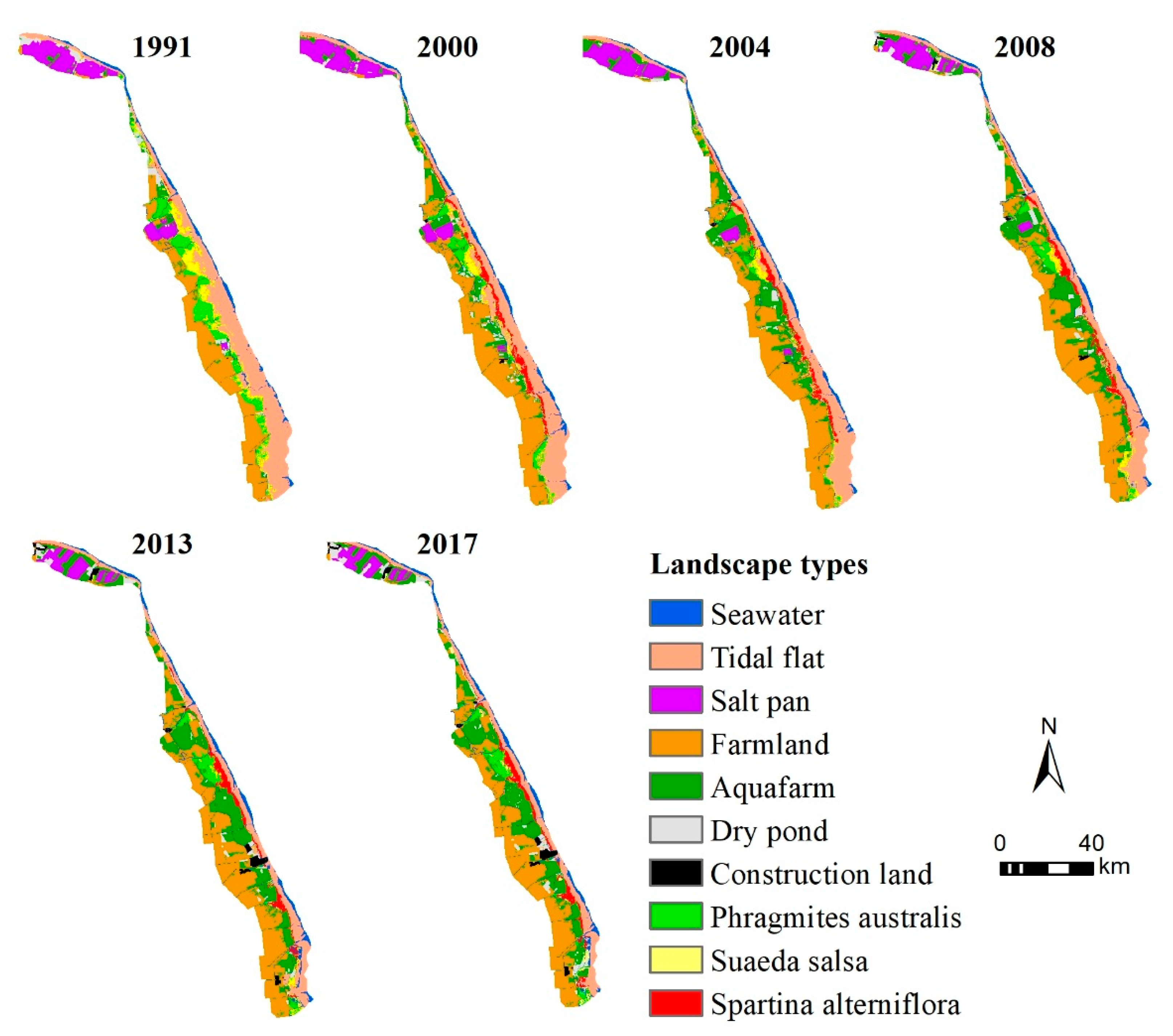
In this study, Landsat Thematic Mapper (TM) and Operational Land Imager (OLI) remote sensing image data were collected from the website of United States Geological Survey (USGS) (http://glovis.usgs.gov/) and the geographic spatial data cloud (reference). There were total 12 scenes of imagery selected from 6 years (1991, 2000, 2004, 2008, 2013 and 2017). Most images were acquired in spring, autumn and winter (from October to May). The basic parameters of the Landsat image data were summarized in Appendix A Table A1. After the multi-year image data were collected, the raw image data were processed with tailing, geometric correction and registration, band synthesis, image embedding and image enhancement. Finally, the processed images were visually interpreted by combining field investigation observations. Accuracies of different landscape types were proved to be higher than 85%. Combining with practical landscape distributions in the City of Yancheng and research needs, landscape types in the present study were divided into natural wetland landscapes and artificial wetland landscapes [39]. The former ones include seawater, tidal flat, Phragmites australis, Suaeda salsa, and Spartina alterniflora. The later ones cover salt pans, farmland, aquafarm, dry pond and construction land (Figure 2). In addition to making use of remote sensing image data, administration boundaries, road traffic, river water systems, planning of Jiangsu Province and the City of Yancheng, data of the natural reserve of Yancheng Coastal Wetland are also needed in landscape simulation for the future scenarios.

2.3. Methods

2.3.1. CA-Markov Model

The CA-Markov model integrates spatial simulation advantages of a CA model and temporal simulation advantages of a Markov model, thus enable to get the probability of occurrence of an event at a moment through spatial simulation [16]. The CA model is a dynamic simulation model in which both space-time and state are discrete and discontinuous. It can solve complicated systems with simple local rules [22]. The expression of CA-Markov model is:
S ( t + 1 ) = f [ S ( t ) ,   N ]
where S is the state set of CA and N is the field range. t and t + 1 are two successive time points. f is the transfer rules of CA state.
The Markov model is mainly used to understand a development trend from one time state to other time states and to predict future development situations according to such variation trends. It has been widely applied to land use simulation [22]. During the land use simulation based on the Markov model, the most important thing is to know the transfer probability ( P i j ) at time point m:
[ P 11       P 12           P 1 n P 21     P 22             P 2 n                                         P m 1     P m 2       P m n ]
On this basis, the land use prediction formula of the Markov model can be gained:
S ( k + 1 ) = S k P = S ( o ) P ( k + 1 )
where S ( k + 1 ) is the prediction results when simulating a land use at t = k + 1 ; S ( o ) is the area of a land use in the beginning of simulation; S k is the prediction results when simulating a type at t = k , and P i j is the probability for transferring type i into type j.

2.3.2. Accuracy Verification of Landscape Simulation

The consistency between the simulated landscape distribution maps and the existing landscape type distribution maps of Yancheng Coastal Wetland in 2017 was tested according to Kappa index. If Kappa > 0.75, the simulation effect is good. If 0.4 ≤ Kappa ≤ 0.75, the prediction result is general. If Kappa ≤ 0.4, the prediction credibility is low [15,21]. The Kappa index is defined as follows:
Kappa = P o P c P p P c , P o = n 1 n       P c = 1 N
where Po is the proportion of accurately predicted grids and Pc is the expected proportion of accurately predicted grids. Pp is generally 1 and it is an ideal prediction value. n is number of grids in a map; n1 is the number of accurately predicted grids, and N is number of landscape types.

2.3.3. Landscapes Ecological Risk Assessment (ERS) Model

The response relation of risk receptors to various development activities by mankind is reflected by changes of landscape types in the study area [40]. With references to a landscape index method, dynamic changes of a regional landscape pattern are reflected clearly by the quantification of corresponding landscape indexes. A landscape interference index ( E i ) and a fragility index ( F i ) were chosen to create the landscape loss index ( R i ), which reflects landscape loss upon external impacts.
R i = E i × F i
where E i is the influence degree of external environment on different landscape types:
E i = a C i + b N i + c D i
where C i is the landscape fragmentation index; N i is the landscape separation index and D i is the landscape dominance index. a, b, and c are corresponding weights. In this study, by referring to previous studies and considering regional characteristics, a, b, and c adopt the values 0.5, 0.3 and 0.2, respectively [41].
In Equation (5), F i reflects the structural stability and fragility of a regional internal ecosystem in the study area. If F i is high, the regional ecosystem has a prominent fragility and poor stability. By referring to Liu [39], ten landscape types were graded from high to low according to the ability to maintain stability upon external impacts: dry pond =10, aquafarm = 9, tidal flat = 8, seawater = 7, farmland = 6, salt pan = 5, Spartina alterniflora = 4, Suaeda salsa = 3, Phragmites australis = 2 and construction land = 1. Finally, F i value was calculated through normalization.
According to the extent of the study area and referring to previous studies [33], a fishing net with appropriately 2–5 times of average patch area in the study area was appropriate. A 2 km × 2 km grid net was constructed using the ARCGIS10.5 fishing net tool and a total of 1010 risk zones were divided in the study area. Combining with R i and area of sampling plot, the calculation formula of ecological risk index was:
E R I i = i = 1 N A k i A k R i
where, in the study area, ERIi is the ecological risk value of landscape type i; Aki refers to the area of landscape type i in the kth sampling zone; and Ak is the area of the kth sampling zone.

2.3.4. Spatial Analysis Method of Ecological Risks

Ecological risk values were given to a center point of risk zones by using the ARCGIS10.3 software. An ecological risk map was generated by running Kriging interpolation with a spatial analysis module [30]. For the convenience of highlighting regional ecological risk changes and conducting a uniform evaluation, the ecological risk index (ERI) value was divided into 7 grades at an interval of 0.10, which are extremely low ecological risk zone (ERI < 0.35), low ecological risk zone (0.35 < ERI ≤ 0.45), relatively low ecological risk zone (0.45 < ERI ≤ 0.55), medium ecological risk zone (0.55 < ERI ≤ 0.65), relatively high ecological risk zone (0.65 < ERI ≤ 0.75), high ecological risk zone (0.75 < ERI ≤ 0.85) and extremely high ecological risk zone (ERI > 0.85).

2.3.5. Multi-Scenario Landscape Simulation and ERS Framework

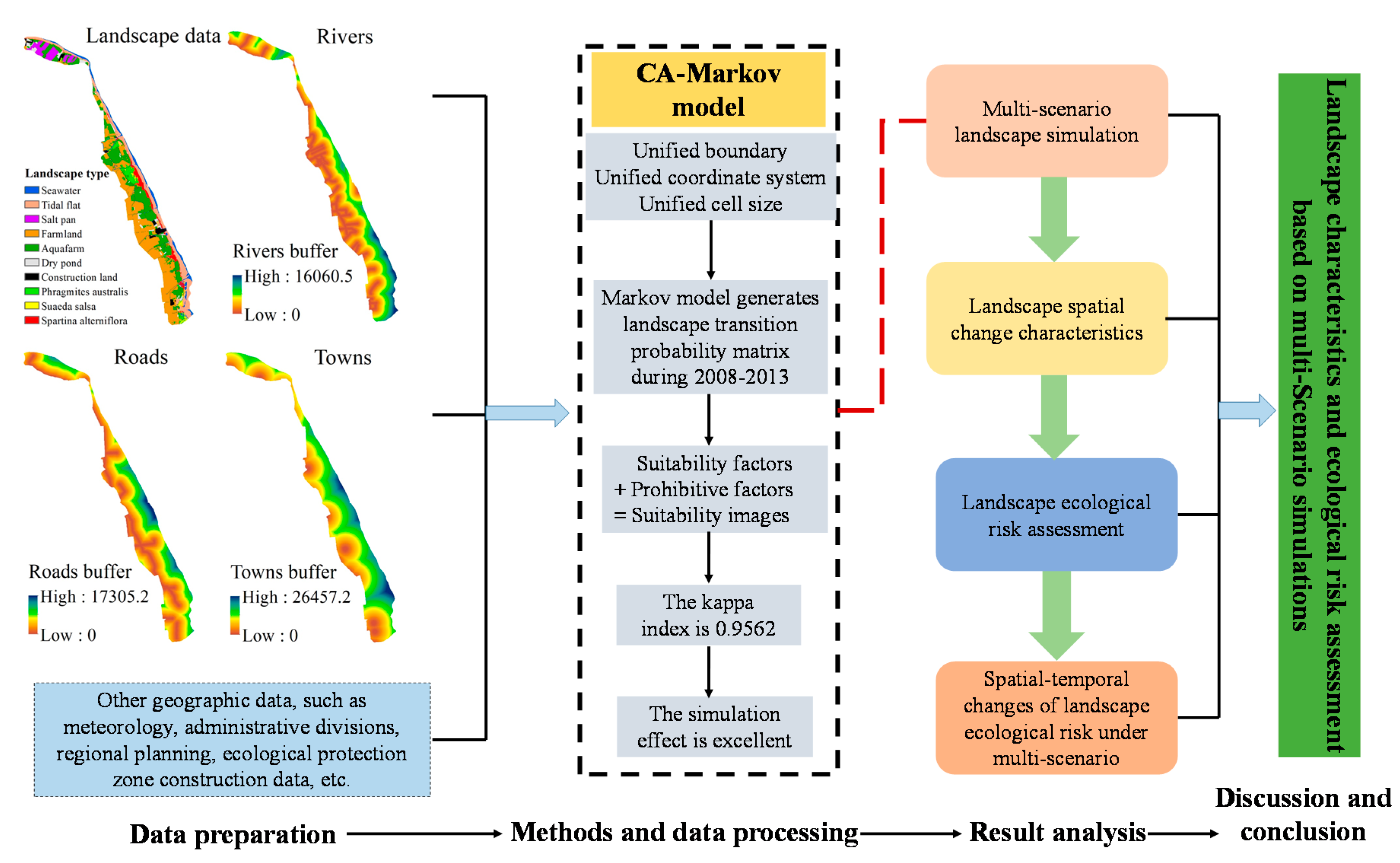
The multi-scenario landscape simulation and ERS framework of coastal wetlands mainly comprised four stages (Figure 3): (1) Data preparation stage, mainly using landscape, river, road, town data, Other geographic data, such as meteorology, administrative divisions, regional planning, ecological protection zone construction data, etc. (2) Method and data processing stage, mainly using CA-Markov model for landscape simulation. (3) Result analysis stage, analyzing the characteristics of landscape changes under multi-scenarios in the region from 1991 to 2025, and conducting landscape ERS on them, and analyzing the characteristics of spatio-temporal changes. (4) Discussion and conclusion stage, Explore the methods of landscape simulation, analyze the reasons for the regional differences of landscape ecological risks, and put forward suggestions for improving the ecological environment.

3. Results

3.1. Multi-Scenario Landscape Simulation Based on CA-Markov Model

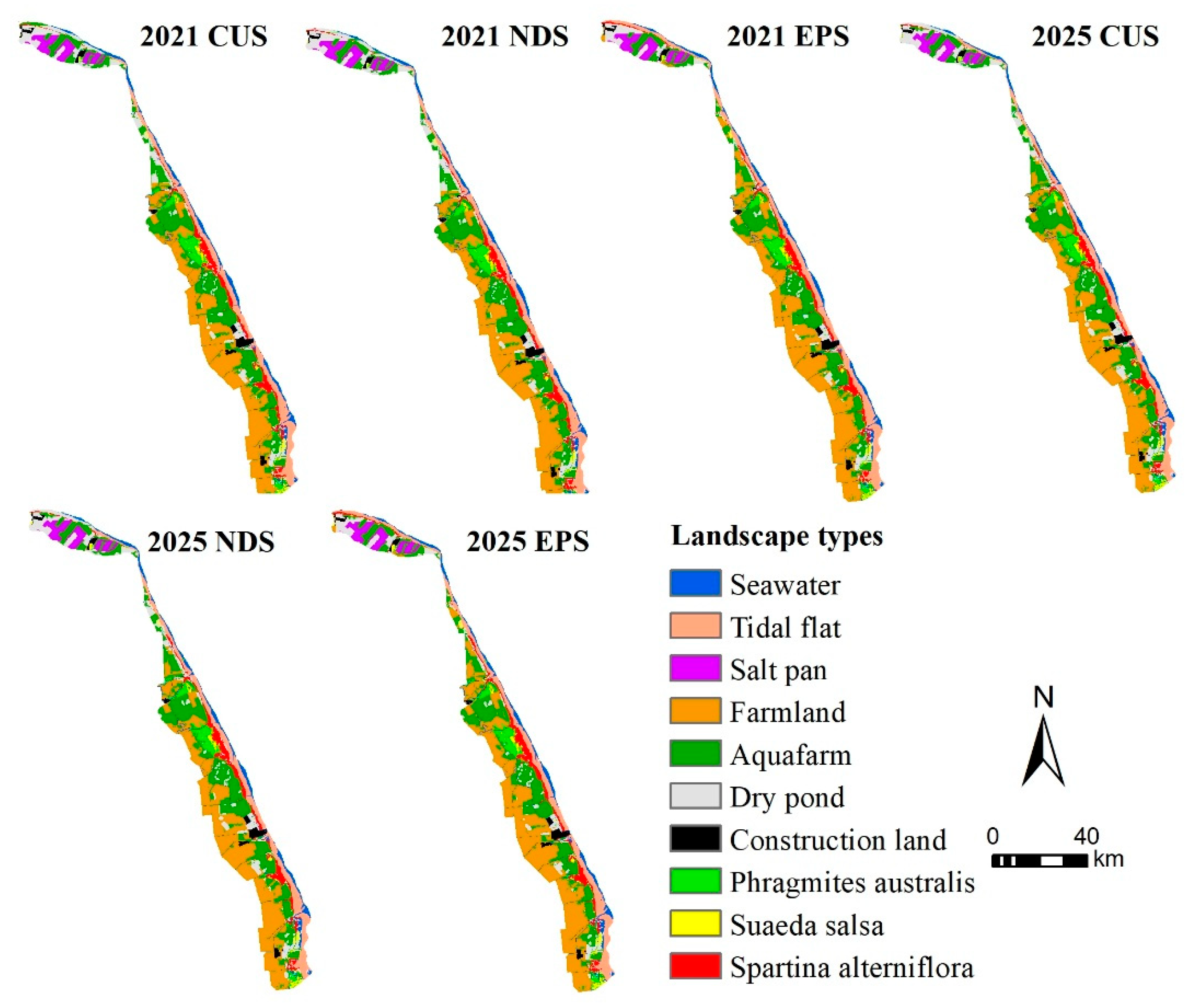
In the present study, three scenarios were hypothesized according to current status of Yancheng Coastal Wetland and government’s requirements on policy planning, which include current utilization scenario (CUS), natural development scenario (NDS) and ecological protection scenario (EPS). Suitability map set and matrices of transfer probabilities were generally different under different scenarios (Figure 4).
(1) CUS: with considerations of history of the study area and landscape changes under current conditions and under a qualified consistence test, constraints and prohibitive factors were chosen for landscape simulation. Hence, the resultant simulation continued and landscape simulation maps of the study area in 2021 and 2025 were gained by iterating the interval of 4 years. This simulation was closer to real landscape data of the study area and this was because it observed the current conditions and basic constraints. It could be called CUS simulation. Taking the transition matrices in 2013 and 2017 as the transition probability, and the 2017 suitability factors such as roads, rivers, towns and related prohibitive conditions as the transition rules, the landscape images of 2021 and 2025 in the current utilization scenario were obtained (Table A2). In this transition probability matrix, dry ponds and fish ponds in artificial wetlands had more conversions, and Phragmites australis, Suaeda salsa, and Spartina alterniflora in natural wetlands had higher conversion probabilities.
(2) NDS: landscape transfer demands of Yancheng Coastal Wetland under NDS mainly referred to transfer probabilities of landscapes during 2013–2017 (Table A2). The landscape transfer observed to landscape transfer laws and rules during 2013–2017, but the landscape changes neglected human activity interference, social economy and policies at present and in future. This was because the landscape transfer in real landscape interpretation maps during 2013–2017 reflected interferences of current human activities and social economy, which formed the map and matrix of real transfer probabilities.
(3) EPS: Given the high construction of ecological civilization, Jiangsu Province and the City of Yancheng published a lot of policies and regulations for protection of Yancheng Coastal Wetland and formulated coastal wetland protection plans successively. Under this background, landscape simulation of Yancheng Coastal Wetland under EPS was mainly to make some changes in matrices of transfer probabilities during 2013–2017, while the suitability map set was kept the same. In the transfer matrix (Table A3), Reducing the outward transfer of natural wetlands, especially to artificial wetland. Hence, the transfer area from natural wetland into construction land was decreased to 0 in the transfer process. Specifically, the conversion of seawater to aquafarm and dry ponds reduced 10,000 hm2 and 557 hm2 respectively. Tidal flats reduced the conversion area to aquafarm (10,000 hm2) and dry ponds (50,000 hm2). The conversion of farmland out of fish ponds and dry ponds has reduced by 60,000 hm2. Phragmites australis reduced the conversion area to aquafarm (177 hm2) and dry ponds (4200 hm2). Suaeda salsa reduced the conversion area to aquafarm (7000 hm2) and dry ponds (3000 hm2). Spartina alterniflora reduced the conversion area to aquafarm (10,000 hm2) and dry ponds (12,000 hm2) [42]. Based on the transfer area matrix gained from transfer reduction and assisted by the suitability map set, the landscape maps in 2021 and 2015 under EPS were gained.

3.2. Landscape Spatial Structural Characteristics of Yancheng Coastal Wetland

There were significant landscape changes in the Yancheng Coastal Wetland. Transfer area, trend, structure and other change characteristics of landscapes in the study area were analyzed by transfer directions of landscape types. Transfer directions were complicated and diversified under the interference of human activities, and the region associated with landscape transfer was extensive in the study area. Hence, the first six landscape transfer types in terms of their greater transfer areas were chosen as research objects to analyze their spatial structural change characteristics.
During 1991–2017, five of the selected six major landscape transfer types were transferred from natural (wetland) landscapes to artificial (wetland) landscapes (Figure 5). On the whole, the transfer area of Yancheng Coastal Wetland was 1770.36 km2, and the transfer probability was 52.03%, indicating an overall frequency of the landscape transfer in the region. There were significant differences among different landscape types. The highest transfer probability was achieved by Suaeda salsa, reaching 79.49%. The tidal flat showed the highest transfer area (693.89 km2), while the construction land had the lowest transfer probability and it was not transferred to other land use types. This fully reflected the transfer differences among different landscape types. With respect to different transfer types, seawater and tidal flat were mainly transferred into aquafarm, Spartina alterniflora and dry pond. The transfer area from seawater and tidal flat into aquafarm mainly concentrated in the north of the wetland, where had high marine development and utilization intensity. Transfer areas from seawater and tidal flat into Spartina alterniflora were close to the core zone of the reserve, and had light or no influences by human activities. As a result, Spartina alterniflora expanded naturally. Salt pan and farmland were mainly transferred to aquafarm and dry pond. There were frequent transfer activities of salt pans in the south of the wetland. Aquafarm was mainly transferred to farmland; dry pond mainly to aquafarm; and both supplemented mutually. Construction lands were slightly transferred to other landscape types at all stages. Tidal flat, farmland and dry pond were used as the main supplementation source of construction land. Phragmites australis and Suaeda salsa were mainly transferred to farmland and aquafarm, which concentrated in the Dafeng District. A small area of Spartina alterniflora was transferred to other landscapes and mainly to tidal flat landscape.
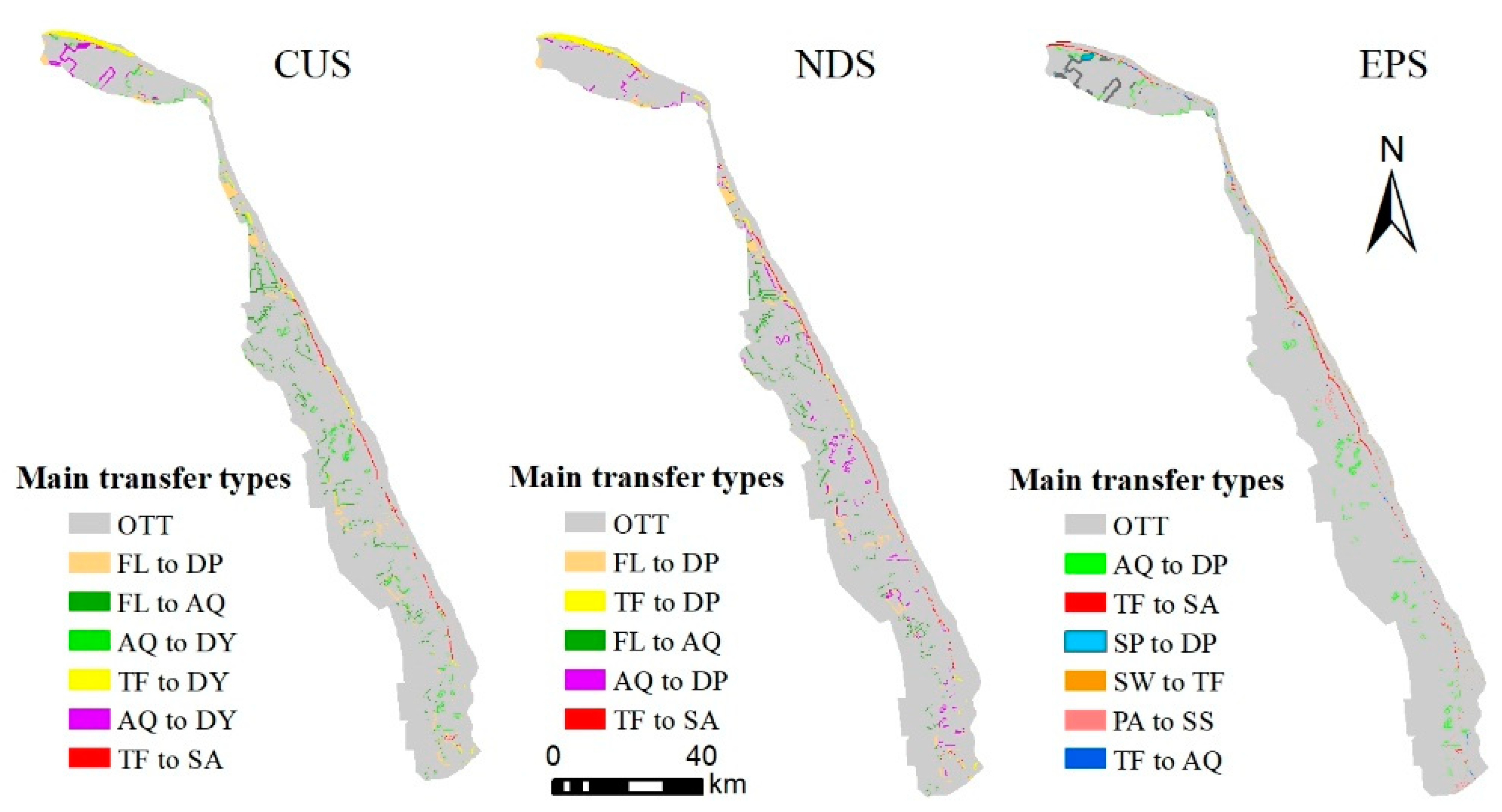
With respect to landscape simulations under different scenarios in future, six types with the greater transfer areas are chosen under CUS scenario, among which five are transfer areas from natural (wetland) landscapes to artificial (wetland) landscapes (Figure 6). Seawater and tidal flat are mainly transferred to aquafarm and dry pond. People use seawater and tidal flat for reclamation aquaculture. The concentrated transfer area from tidal flat to dry pond is in coastal zones of Shangshui County, where is accompanied with concentrated transfer area from aquafarm to dry pond. Besides, there is large-scaled transfer area from tidal flat to Spartina alterniflora, which is mainly in coastal regions on the south of the middle road in Sheyang County. Salt pond is mainly transferred to dry pond, while farmland is mainly transferred to aquafarm and dry pond, which concentrates in the Dafeng District. There are small transfer areas of dry pond, construction land, Phragmites australis, Suaeda salsa and Spartina alterniflora. However, Phragmites australis, Suaeda salsa and Spartina alterniflora in the ecological wetland are mainly transferred to aquafarm and dry pond. Under NDS, four of the five selected landscape transfer types are from natural wetland to artificial wetland. Areas of dry pond and aquafarm increase significantly, while areas of Phragmites australis, Spartina alterniflora and Suaeda salsa decline. Under EPS, 3 of the selected 6 main landscape transfer types are from artificial wetland into natural wetland. Compared to NDS scenario, EPS scenario achieves some landscape ecological protection effect. The salt pan shows the highest transfer probability (16.99%), followed by seawater, Phragmites australis, tidal flat and aquafarm. Transfer probabilities of other landscape types are relatively low. The transfer area of aquafarm is the highest, reaching 66.19 km2. Spartina alterniflora and Suaeda salsa have the smallest transfer areas, which are only 1.90 km2 and 2.11 km2, respectively. Spatially, the total transfer area of different landscape types under EPS is relatively small (201.23 km2) and the transfer probability is only 5.91%. This reflects that the landscape transfer tends to be stable and the landscape structure tends to be simple. The dry pond presents the biggest areal change in the north, while areas of Spartina alterniflora in the center and south changes quickly.

3.3. Landscape Ecological Risk Assessment of Yancheng Coastal Wetland

Combining with ecological risk index, ecological risk values of different years and different sampling zones were gained. Moreover, spatial distribution maps of ecological risks of Yancheng Coastal Wetland were created by linking center points of sampling zones and by using the Kriging tool under spatial analysis in ArcGIS. In addition, statistics on zone area with different ecological risk grades at different stages were carried out and used to analyze spatiotemporal changes of ecological risk in the study area under different scenarios at different stages.

3.3.1. Spatiotemporal Change Characteristics of Landscape Ecology

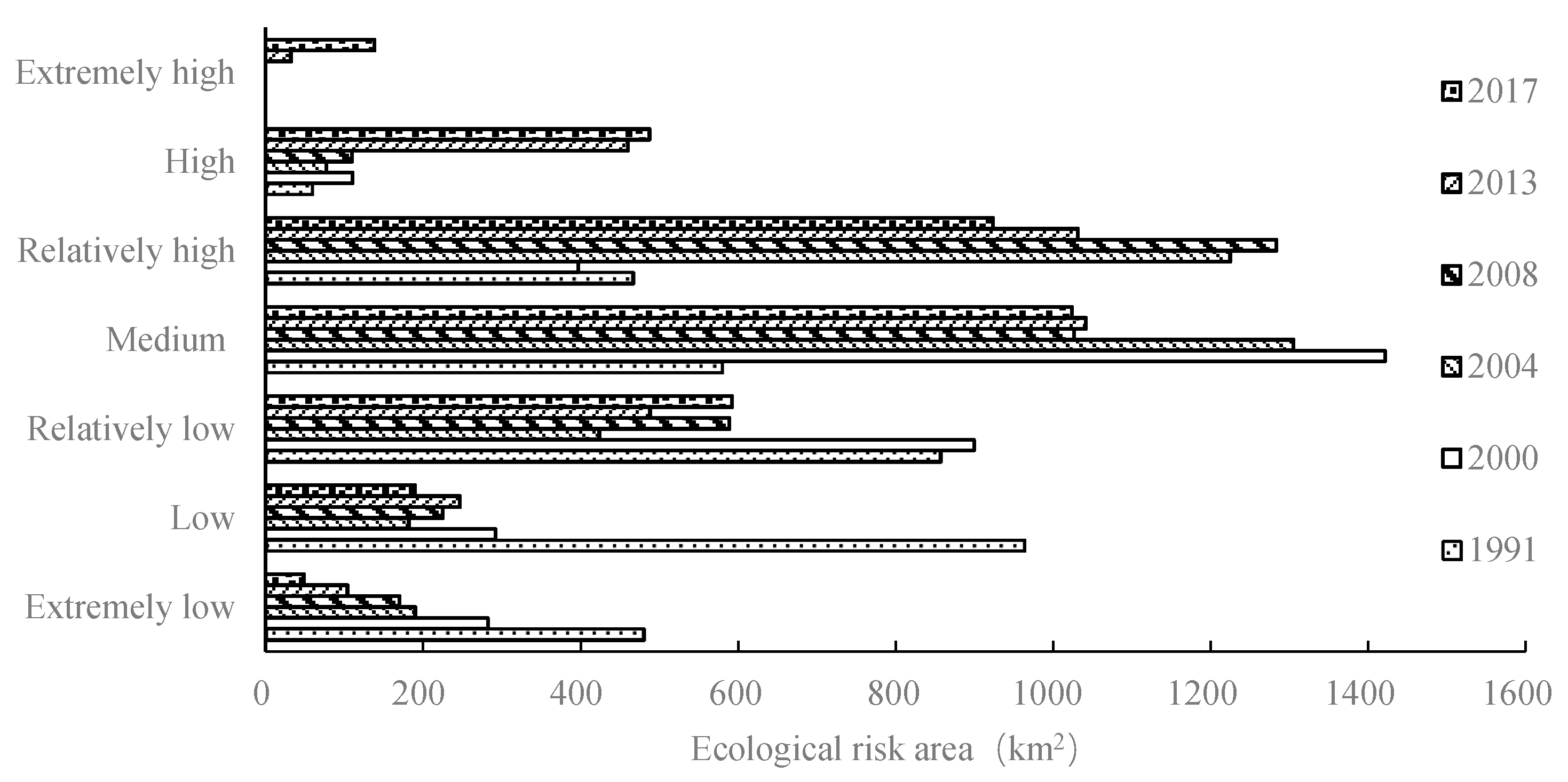
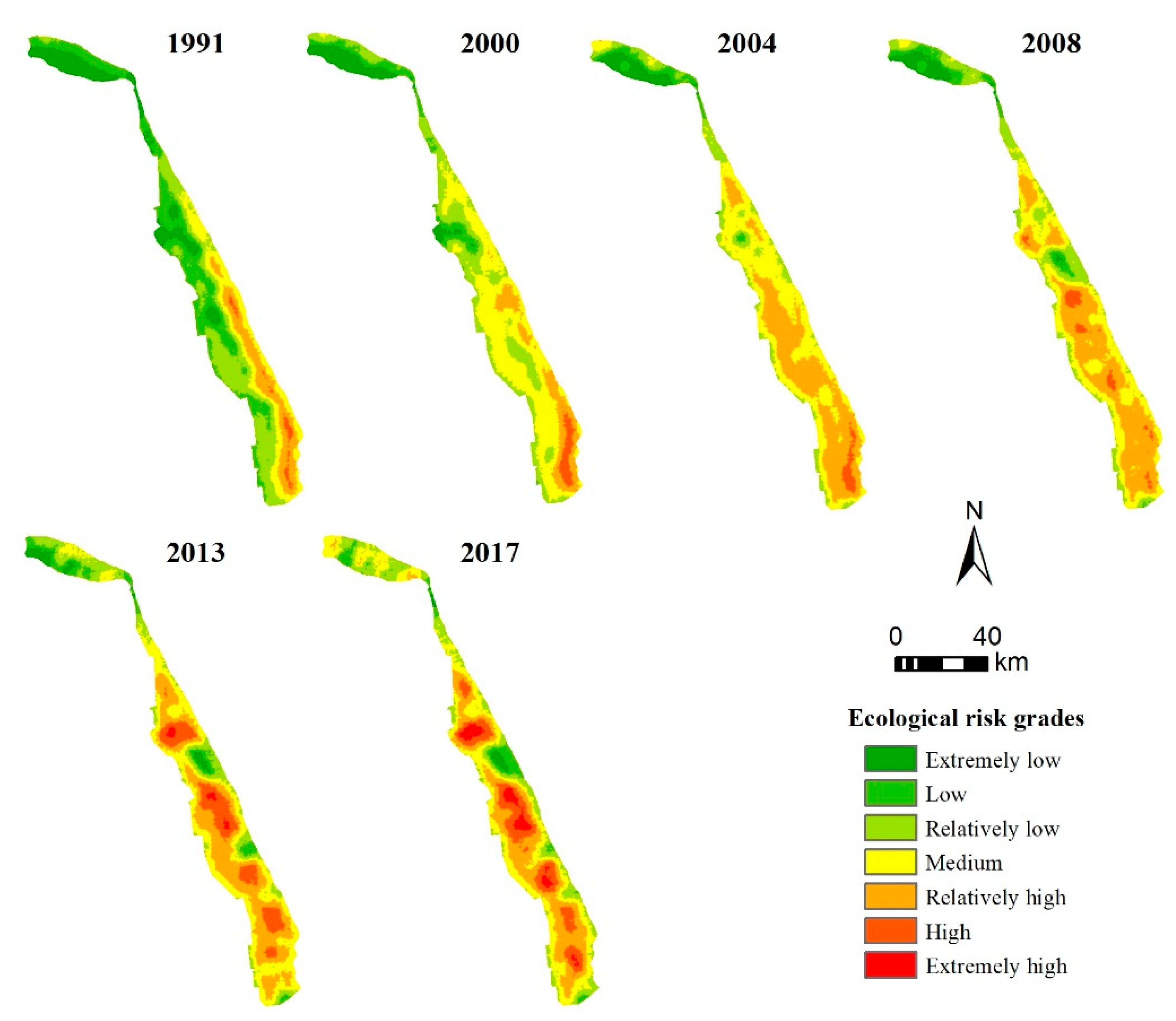
Analyzing the spatio-temporal distribution of ecological risks in Yancheng coastal wetlands and the areas of risk areas at different levels, (Figure 7 and Figure 8), the ecological risk level was increasing over time. It increased from 6 risk grades during 1991–2008 to 7 risk grades in 2013. The area of extremely low risk zone declined quickly by 89.87% (431.07 km2). The maximum reduction rate was during 1991–2000, which led to the extremely low risk zone shrank quickly. Subsequently, the reduction rate became stable. The changes of areas of low risk zone and extremely low risk zone were similar. It decreased by 80.27% (772.61 km2) compared to that nine years ago. It decreased by 69.66% (670.46 km2) during 1991–2000. The area of relatively low risk zone declined less and was by 30.92%, and the relatively high reduction amplitude occurred between 2000 and 2004. The areas of medium, relatively high and high risk zones increased by 76.79% (444.59 km2), 98.09% (457.18 km2) and 731.10% (428.50 km2), respectively. These also demonstrated intensive ecological risks in the Yancheng Coastal Wetland. The medium risk zone achieved a sharp growth by 842.23 km2 during 1991–2000, followed by a slow reduction. The area of relatively high risk zone decreased firstly and then soared up, and finally decreased at a stable rate. It increased quickly by 827.80 km2 during 2000–2004. The area of high risk zone increased by 428.50 km2 during the 26 years. The area of extremely high risk zone increased from zero until it increased by 106.10 km2 during 2013–2017. By considering temporal change characteristics of ecological risk zones in the Yancheng Coastal Wetland, areas of extremely low, low, and relatively low risk zones decreased quickly, while areas of medium, relatively high, high and extremely high risk zones increased dramatically. Therefore, the Yancheng Coastal Wetland was facing great ecological risk threats.
Ecological risks showed significant spatial distribution differences (Figure 8). Ecological risk was low in north part and high in south part in the study area at all 6 stages. Bordered at the center of Sheyang County, there were significant differences between south and north regions, which were expanding continuously. Ecological risks tended to increase. Ecological risk also presented great spatial differences across land-to-coastal transition. During 1991–2004, ecological risk presented a stripped growth from land to coastal regions and the ecological risk in land area was lower compared to that of coastal areas. During 2008–2017, ecological risks were high in middle and low in surrounding areas and ecological risks decreased gradually from central areas to land and coastal areas. Extremely low, low and relatively low ecological risk areas concentrated in the northern of Yancheng Coastal Wetland. Medium ecological risks concentrated in southern zone. High ecological risk zones, including relatively high, high and extremely high levels, mainly concentrated in the southern of Sheyang County. They were transferring from coastal regions to inland regions gradually.
At different time stages, ecological risk of Yancheng Coastal Wetland was mainly low in 1991 and low ecological risk zones concentrated in north and inland areas. In 2000 and 2004, the medium ecological risk zones took the dominant role. The relatively high and high ecological risk zones expanded, while low ecological risk zones concentrated in north region of Binhai County. However, the low ecological risk zone on the inland side was replaced by the zones of the next risk grade. In 2008, the relatively high ecological risk zones took the dominant role and concentrated in the economically developed southern zone. During 1991–2008, ecological risks in southern coastal regions of were relatively high, which were mainly attributed to the increased development of coastal regions in Jiangsu Province. All constructions of coastal towns and modernized facilities, such as coastal industrial parks, foreign trade industry and international logistics, intensified the landscape use and transfer and increased ecological risk levels in the study area. During 2013–2017, there were extremely high ecological risk zones, mainly related to aquafarm. The large-scaled distribution of aquafarm and construction of relevant facilities formed the extremely high ecological risk zones centered at aquafarm. Moreover, ecological risks decreased gradually from the center to surrounding areas.

3.3.2. Spatiotemporal Change Characteristics of Landscape Ecological Risks under Multi-Scenario

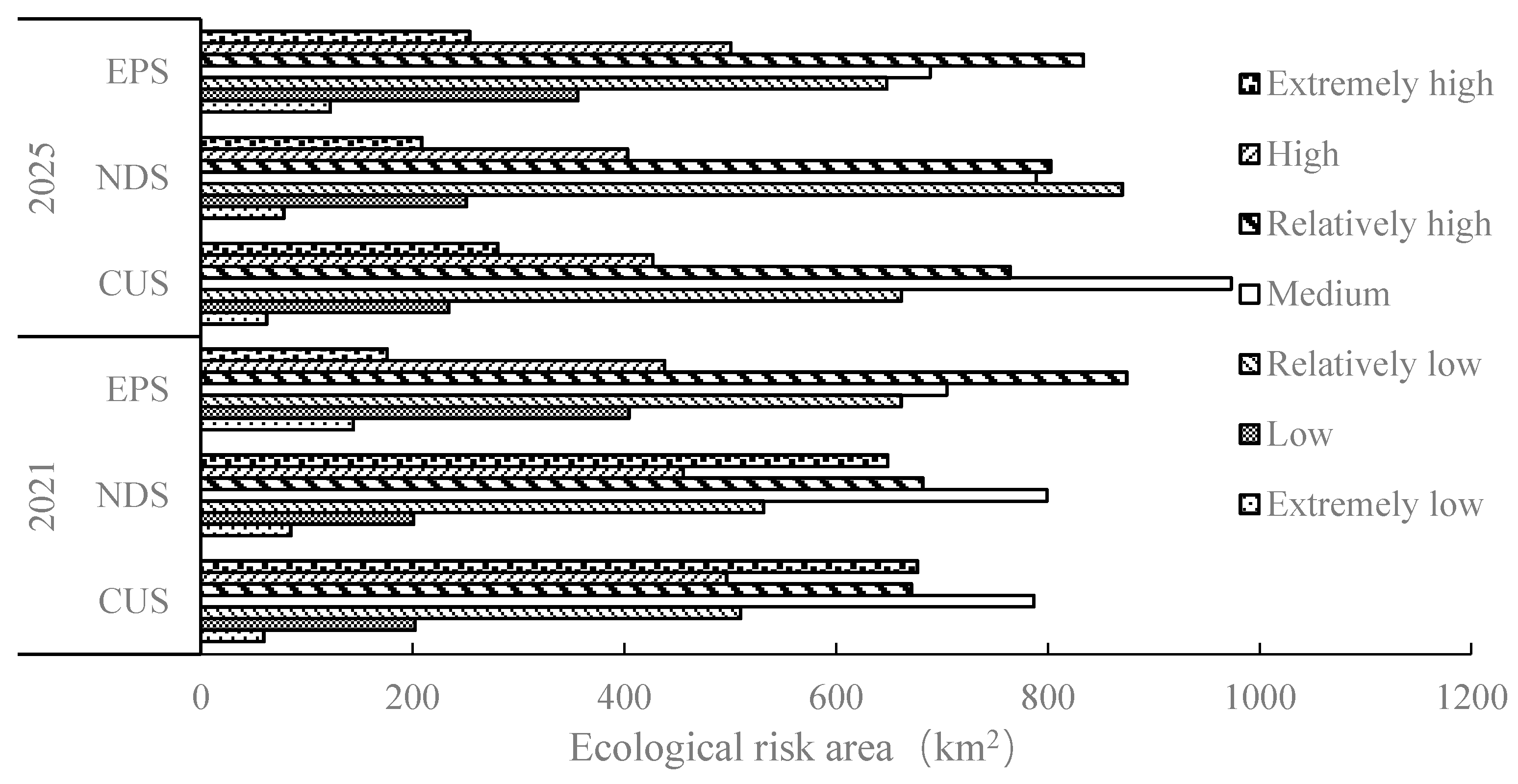
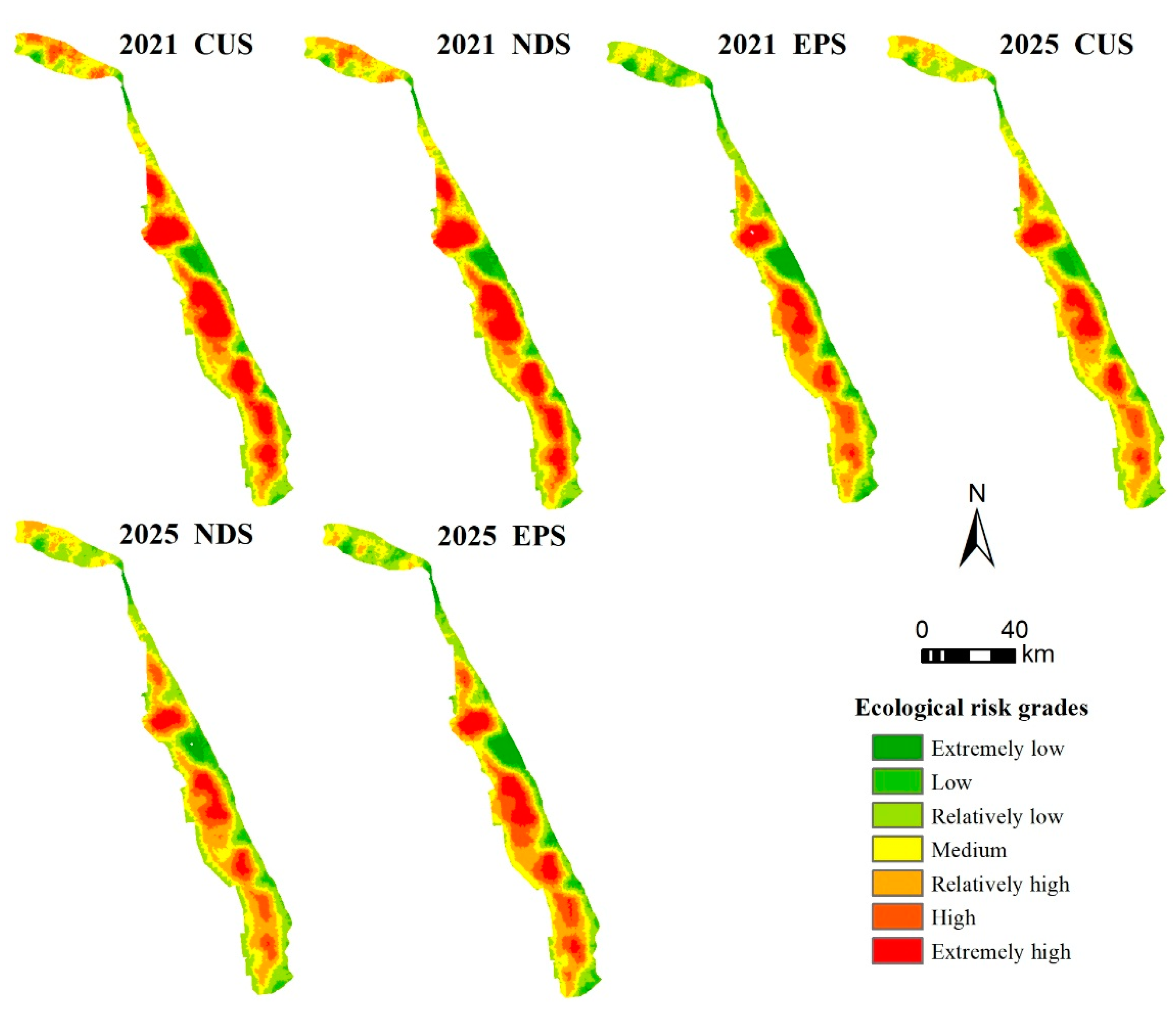
Landscape maps of Yancheng Coastal Wetland in future under different scenarios were gained through the landscape simulations. The spatial distribution maps of ecological risks under three scenarios during 2021–2025 were generated by interpolating ecological risk index and calculating statistics on ecological risk areas. On this basis, temporal and spatial change characteristics of ecological risks in future under the different scenarios were analyzed (Figure 9 and Figure 10).
Under CUS scenario, the medium ecological risk zone takes the dominant role over time. The area of extremely high ecological risk zone increases by 142.19 km2, while the areas of high, relatively high and medium ecological risk zones decline. The areas of extremely low, low and relatively low ecological risk zone increase slowly. These demonstrate that under CUS, the current accessibility factor and ecological protection measures can relieve the overall ecological risks of the Yancheng Coastal Wetland in 2025 although the extremely high ecological risk increase. Under NDS scenario, the dominant ecological risk level increases from medium in 2021 to relatively high in 2025. The area of the extremely high ecological risk zone under NDS increases slightly compare to that under CUS. Moreover, the areas of extremely low, low and relatively low ecological risk zones increase significantly, and the areas of high, relatively high and medium ecological risk zones decrease gradually. All these reveal that the NDS which conforms to internal landscape transfer laws of the Yancheng Coastal Wetland achieves greater ecological protection effectiveness than CUS. Under EPS scenario, the dominant ecological risk is changed from the relatively high risk grade in 2021 to the medium risk grade in 2025. Under ecological protection control, landscape transferring into artificial wetland area decreases significantly, which decreases the area of high ecological risk zone and expand the low ecological risk zone into the high ecological risk zone. Specifically, the areas of extremely low, low and relatively low ecological risk zones are increased by 73.75 km2, 166.05 km2 and 55.87 km2 compare to those in 2017. The area of extremely low ecological risk zone increases with mostly showing a great growth rate of 151.75%. The areas of medium and relatively high ecological risk zones decline, while the areas of high and extremely high ecological risk zones increase, but the increased amplitude is relatively lower compare to that under CUS. By combining three scenarios, ecological risks are controlled and relieved to some extent. The areas of high ecological risk zone under CUS and NDS are significantly higher than that under EPS. This also proves the importance of ecological protection to control and weaken ecological risks as well as the necessity of observing natural development laws and formulating new ecological protection policies.
Per the spatial distributions, high ecological risk zones concentrated in southern Sheyang County under three scenarios (Figure 10). Regions with a low ecological risk concentrate in the long narrow region of Binhai County as well as the core zone. The low ecological risk zone in the northern region transferred to relatively low and medium ecological risk zones. In the north region with a rapid economic development, salt pan was still a dominant landscape type. However, occurrences of dry pond and aquafarm in simulated landscapes occupied certain areas of salt pan and tidal flat, thus increasing ecological risks in the northern region. Aquafarm was a main landscape type in the high ecological risk zone. Yancheng Coastal Wetland is close to the Yellow Sea and local rivers that mainly flow from the west to the east into ocean. There were abundant nutrients in intersections of rivers, which were appropriate for development of large-scaled fishery aquaculture and convenient for water conservancy constructions. The large-scaled increase of aquafarm increased uses of tidal flat, Phragmites australis, Spartina alterniflora, Suaeda salsa and farmland, thus resulting in occurrence of high ecological risk zones. Under CUS and NDS, the scope of high ecological risk zone in 2021 is larger than that in 2025. High and relatively high ecological rick zones occur in Shangshui County and Binhai County in 2021, which are transferred to medium, relatively low and low ecological risk zones in 2025. In the southern coastal regions, the low, relatively low, medium and relatively high ecological risk zones advance toward the land side, indicating that marine development in 2025 is more reasonable and ordered. Under EPS, the extremely low, low and relatively low ecological risk zones expand. Compared to the situations in 2017, the low ecological risk zones are under good protection, while the medium, relatively high, high and extremely high risk zones are controlled to some extent.
By considering spatio-temporal changes of ecological risks under the three scenarios, the ecological risk under CUS is more serious compared to those under NDS and EPS. During 2017–2025, EPS plays a key role in inhibiting ecological risks. Therefore, the extremely low, low and relatively low risk zones under EPS are expanded, while the medium, relatively high, high and extremely high ecological risk zones are decreased, thus controlling ecological risk of the region effectively. For example, a core zone is constructed, where human activities are prohibited completely and landscapes follow natural development. As a result, the ecological risk in the region centering at the core zone is relatively low. This also suggests to observe natural development of landscapes and decrease interferences of human activities under implementation of ecological protection policies, such as a reclamation of tidal flat, occupation of vegetation and farmland for construction activities, damages to complete landscape patches by road construction, etc.

3.3.3. Transfer Changes of Landscape Ecological Risks

Statistics on transfer directions of large-scaled ecological risks in different years were carried out, which is conducive to analyzing annual average rate of coastal wetland transfer directions and reflects diversity and complexity of an ecological risk transfer. Six time periods during 1991–2017 and three scenarios for landscape simulations during 2017–2025 were chosen.
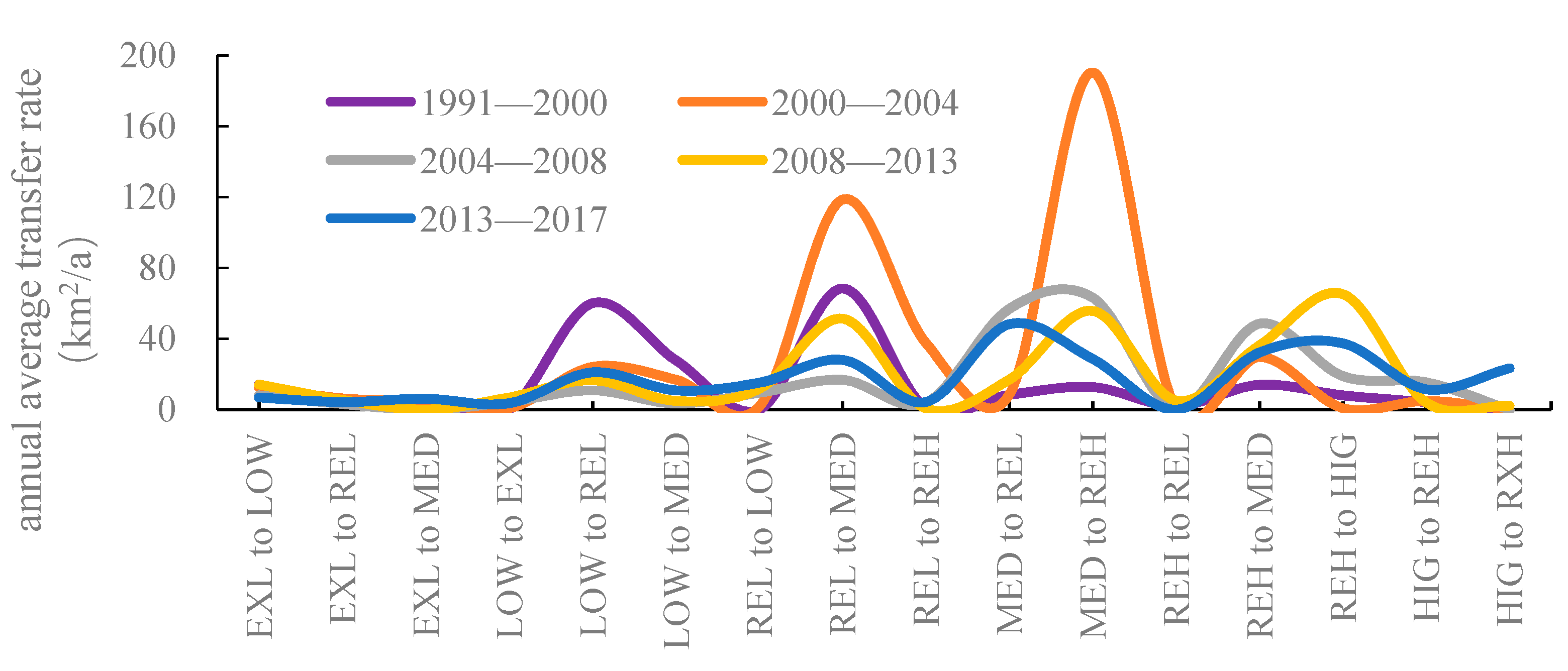
There were 35 transfer directions of ecological risks during 1991–2017. The total transfer area from a low ecological risk level to a high level could account for 2473.34 km2, which was 4.35 times that of the total transfer area from a high level to a low level (569.12 km2). This fully demonstrated the transfer complexity of ecological risks of Yancheng Coastal Wetland as well as the intensive impacts of rapid urbanization and industrialization on regional ecological risks. In the present study, a total of 16 landscape types with greater transfer areas were chosen for analysis (Figure 11). The annual transfer rates of five types, namely, EXL–LOW, LOW–REL, LOW–MED, REL–MED and REH–REL declined gradually. The transfer direction was mainly from low to high. The annual average rates of 11 transfer types, including EXL–REL, EXL–MED, LOW–EXL, REL–LOW, REL–REH, MED–REL, MED–REH, REH–MED, REH–HIG, HIG–REH, and HIG–EXH, increased gradually and the main transfer direction was from low to high. This demonstrated that regional ecological risk transferred from low to high and high ecological risk zone was expanded significantly. Among these transfer directions, two major peaks occurred in the REL–MED and MED–REH during 2000–2004, with a rate of 118.59 km2/year and 190.41 km2/year.
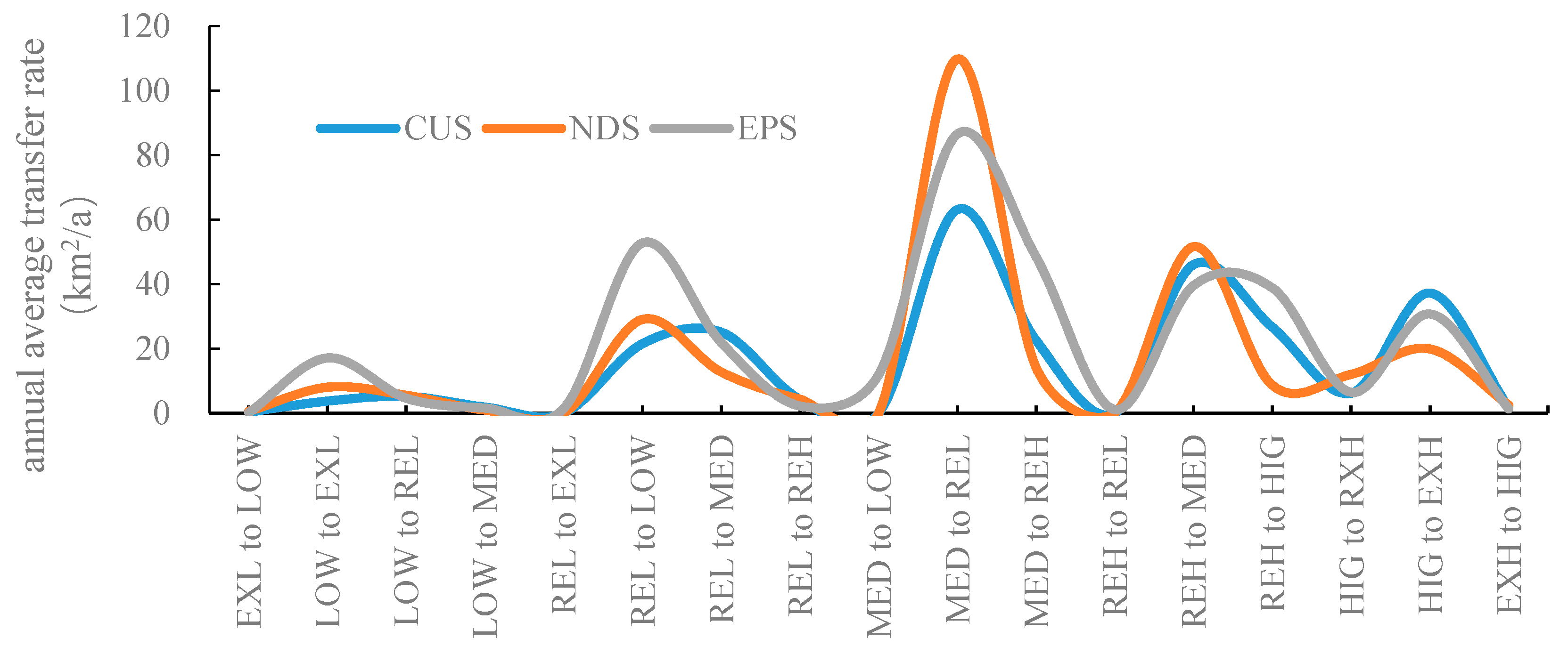
During 2017–2025, there were 24 transfer directions in statistics under the three scenarios, which decreased by 9 compared to that during 1991–2017. The ecological risk transfer was relieved. In this study, fifteen main transfer directions were chosen (Figure 12). Among them, the annual average rates of EXL–LOW, LOW–REL, LOW–MED, REL–MED, REL–REH, REH–MED, HIG–EXH, and EXH–HIG declined and the main transfer direction was from low to high. The annual average rates of LOW–EXL, REL–EXL, REL–LOW, MED–LOW, MED–REL, MED–REH, REH–REL, REH–HIG and HIG–REH increased and the main transfer direction was from high to low. Similar fluctuations are observed at different transfer directions under the three scenarios, with a general consistence between peaks and valleys. There are five obvious peak points, which are LOW–REL, REL–LOW, MED–REL, REH–MED, and HIG–EXH. Under NDS, the maximum peak zone is in the medium-relatively low zones and the annual average transfer rate is 109.89 km2/year. Peak values are mainly transferred from high to low ecological risks. This reflect that under the simulation scenarios, ecological risks of Yancheng Coastal Wetland are controlled and decreased effectively by implementation of ecological protection policies as well as reasonable development and use of landscapes. This also suggests to strengthen ecological restoration and protection of wetland in future, implement current ecological protection policies, formulate new planning policies according to new environment in future, and promote high-efficiency and reasonable use and protection of coastal wetlands.

4. Discussion

4.1. Applications and Improvement of Landscape Simulation Methods

Based on data acquired in 2008, 2013 and 2017, appropriate important influencing factors of landscape changes in Yancheng Coastal Wetland were chosen. Suitability factor and prohibitive factor were combined as the transfer standard. The transfer probability maps which were generated based on landscape data collected in 2008 and 2013 were used as transfer probabilities to generate the simulated landscape maps in 2017. According to the accuracy verification, Kappa index reached 0.9562 in this study, indicating that the chosen factors and methods tended to be reasonable and scientific. Hence, the CA-Markov model was applied to create landscape data of Yancheng Coastal Wetland in 2021 and 2025. This also proved feasibility, practicability and reasonability of the CA-Markov model in temporal and spatial simulations. Since the artificial interferences have been existed in the key wetland reserve of Yancheng Coastal Wetland in Jiangsu Province, there are great regional differences of interference forces in the study area. Studies on landscape changes under influences of internal and external environments have different expression forms in different periods. In the study area, external impacts were weakened, while internal impacts were strengthened. Therefore, most of selected factors were internal influencing factor and external factors were mainly accessibility factors.
Map data in a specific period in future were gained through simulation with the CA-Markov model. Current natural, social and economic factors were considered in the simulation process. Continuity of these factors should be discussed. For example, continuity or sudden interruption of influences of policies and planning and acting forces of different factors have to be discussed independently for different landscape types. In addition, climatic changes, seawater erosion and settlement changes in the study area were neglected due to difficulties in data accession. Although the landscape simulations for future scenarios offset uncertain factors of current policies, simulation accuracy still could be improved. This indicates that it is inevitable to have some error between the simulated landscape data and real landscape data. However, such error is controllable. Hence, an idea simulation needs various supports from multisource data so that it can simulate landscape changes in a study region more accurately.

4.2. Spatial-Temporal Distribution Differences of Landscape Ecological Risks

The ecological risk differences between south and north regions were closely related with economic development differences in the Yancheng City spatially. Economic development levels in the south region are significantly higher than those in the north region. In north regions of the study area, economic development is focused on production of salt pan. Therefore, landscape types mainly include simple salt pan and human utilization intensity of landscapes is limited. During 1991–2008, the study area was mainly occupied by the extremely low and low ecological risks, but it was increased to the medium ecological zone during 2013–2025. The ecological risk level has been kept at a relatively high level, which was mainly caused by the significantly higher economic development strength in the south region than that in the north region. There exist dense distributions of rivers in the south region and most estuaries of rivers are ports, which have a frequent connection with their external environments through rivers and sea ports. The south shoreline belongs to the deposit type and the tidal flat occupies extensive areas. The intensity of making use of the tidal flat by human increased continuously. The culture pond extended continuously toward sea side, thus resulted in continuous constructions of water conservancy facilities for irrigation canal series, road network facilities, service facilities and power facilities which are needed for daily life. Such continuous constructions significantly occupied tidal flat, farmland and vegetation lands. There’s a high urbanization level in the south region and population increased significantly in coastal cities and towns due to merging village and towns. However, the practical construction land use area didn’t increase greatly, but the improved urbanization frequently brought out landscape transferring activities. Landscapes transferred quickly as a result to economic development in south regions, which resulted in the high ecological risk level in the south region of the study area.
Ecological risk differences between land and coastal areas are significantly related with economic development and current policies. Ports in coastal regions have obvious advantages, which have brought out constructions of relevant industries and infrastructures and increased utilization degree and transferring rate of landscapes. In particular, the rapid marine economic development in early years also increased the development and utilization intensity of coastal zones. Hence, the landscape utilization level of human activity in coastal regions was relatively higher than that in inland, which was relatively obvious in spatial distribution of ecological risk during 1991–2004. In addition to the economic development, government policies can influence ecological environment significantly. During 2008–2025, the ecological risk level at the outer edge of the Coastal Wetland began to decline and transfer to the relatively low, low and extremely low ecological risk zones. In particular, the border area between Sheyang County and Dafeng District was divided as a core zone by the protection area of the Wetland. In 2008, the local government adjusted the core zone, test zone and buffer zone. The area of the core zone was increased by 4600 ha. Besides, it regulates that human activities are prohibited completely in the core zone and the regional ecosystem shall be protected strictly to follow natural growth and development. This measure efficiently relieves ecological risk of the region and promotes restoration and stability of the ecosystem.
The current government is increasing protection strength to Yancheng Coastal Wetland continuously. Hence, ecological risks of simulated landscapes under the three scenarios tend to decline. Specifically, the ecological risk under EPS is the lowest, followed by those under CUS and NDS successively. This also proves the importance and urgency of formulating ecological protection policies to control ecological risk in coastal wetlands. Moreover, it is suggested to observe natural development laws of coastal wetland landscapes and control external interferences of human activities, and thus promote the sound cyclic development of ecosystem in coastal wetlands.

5. Conclusions

Based on multi-year remote sensing images, road traffics, rivers and other basic data of Yancheng Coastal Wetland, China, spatial distribution data of landscapes under three different scenarios in future were simulated by using the CA-Markov model. Ecological risks of different landscape types in the coastal wetland were assessed by an ecological risk index. On this basis, differences of spatiotemporal characteristics of ecological risks of coastal wetlands were analyzed. The analysis results are expected to provide some theoretical and practical references to ecological environmental protection and sustainable development of Yancheng Coastal Wetland. Some major conclusions could be drawn from the analysis results:
(1) The test accuracy of the CA-Markov model was relatively high and it passes through the consistency check. Simulation results could be divided into CUS simulation, NDS simulation and EPS simulation according to the simulation process. During 1991–2025, there are complicated landscape transfers and extensive transfer regions in the Yancheng Coastal Wetland. The total transfer area can be 1770.36 km2. Regions with violent landscape transfers concentrate in south central regions of the Sheyang County. Under CUS and NDS scenarios, transfer area from natural wetland to artificial wetland increases. Under EPS, the area of artificial wetland declines and it is mainly transferred to natural wetland. The landscape structure tends to be stable.
(2) During 1991–2017, ecological risks were intensified and the spatial differentiation was obvious. Low ecological risk zones shrank quickly, while high ecological risk zones expanded significantly. With respect to spatial distribution, ecological risks presented low in the north and high in the south. Bordered at the central area of Sheyang County, the gap between the south and the north was large and it was expanding continuously. There were also some differences between sea areas and land areas. During 2017–2025, the medium ecological risk zone takes the dominant role under CUS, while the ecological risk level is improved under NDS. On contrary, the ecological risk level declines under EPS.
(3) During 1991–2017, there were significant transfers of ecological risks. The transfer area from low to high ecological risks was 4.35 times that from high to low ecological risks and the transfer directions of ecological risks were up to 35. The peak points of the transfer rate concentrated at the REL–MED and MED–REH during 2000–2004. There are 24 transfer directions during 2017–2025 and five prominent peak points of the transfer rate under the three scenarios, which are LOW–REL, REL–LOW, MED–REL, REH–MED, and HIG–EXH.

Author Contributions

Conceptualization, P.T. and J.L.; methodology, P.T., H.G. and L.C.; software, P.T. and C.L.; validation, P.T., and J.L.; data curation, L.C. and C.L.; writing—original draft preparation, P.T.; writing—review and editing, L.C. and R.P.; All authors have read and agreed to the published version of the manuscript.

Funding

This research was funded by the NSFC-Zhejiang Joint Fund for the Integration of Industrialization and Informatization (U1609203), National Natural Science Funded project (41976209, 41771199).

Acknowledgments

The authors hope express their gratitude to the editors and the anonymous reviewers for providing valuable comments and suggestions to improve the paper.

Conflicts of Interest

The authors declare no conflict of interest.

Appendix A

Table A1. A summary of basic parameters of Landsat image data.
SatelliteSensorsPath/RowDate (yy-mm-dd)SatelliteSensorsPath/RowDate (yy-mm-dd)
Landsat5TM120/361991-11-19Landsat5TM119/371991-11-28
Landsat5TM120/362000-12-13Landsat5TM119/372000-12-06
Landsat5TM120/362004-12-08Landsat5TM119/372004-11-15
Landsat5TM120/362008-12-19Landsat5TM119/372009-01-13
Landsat8OLI120/362013-12-01Landsat8OLI119/372013-12-10
Landsat8OLI120/362017-12-01Landsat8OLI119/372017-12-10
Table A2. Transition probability matrix of current situation utilization and natural development scenarios.
Landscape TypesCalss1Calss2Calss3Calss4Calss5Calss6Calss7Calss8Calss9Calss10
Calss10.86040.05320.00000.00020.05090.00210.00000.00480.00970.0186
Calss20.00160.77550.00000.00000.03520.10800.00000.00780.01010.0618
Calss30.00000.00000.83190.00000.00000.16670.00010.00000.00000.0012
Calss40.00010.00000.00000.89030.05000.05480.00000.00040.00430.0001
Calss50.00010.00020.00000.00030.87390.10830.00000.00040.00430.0041
Calss60.00030.00020.00000.00020.20750.76110.00010.00650.00660.0041
Calss70.00000.00060.00000.00000.00060.00480.89580.00000.07510.0232
Calss80.00050.00020.00000.00000.00120.03230.00080.86580.05700.0422
Calss90.00080.00080.00000.00020.16040.07000.00750.00520.67460.0805
Calss100.00110.00120.00000.00000.07330.08300.00030.00140.00480.8348
Note: Calss1: Seawater; Calss2: Tidal flat; Calss3: Salt pan; Calss4: Farmland; Calss5: Aquafarm; Calss6: Dry pond; Calss7: Construction land; Calss8: Phragmites australis; Calss9: Suaeda salsa; Calss10: Spartina alterniflora.
Table A3. Changes in the area of landscape transfer in ecological protection scenarios.
Landscape TypesCalss1Calss2Calss3Calss4Calss5Calss6Calss7Calss8Calss9Calss10
Calss1225,02913,91605513,3105573126325444857
Calss2806396,5431717,97555,22273988517331,609
Calss304130,8830626,2211802189
Calss4171001,121,15462,99369,024104725398101
Calss5851524250832,141103,09267617862943834
Calss6503833539,611145,3142320945523212
Calss7044004437770,060058711817
Calss86728001774732120126,86183506189
Calss938390107699335835825032,3833866
Calss101882090012,71214,39154238831144,691
Note: Calss1: Seawater; Calss2: Tidal flat; Calss3: Salt pan; Calss4: Farmland; Calss5: Aquafarm; Calss6: Dry pond; Calss7: Construction land; Calss8: Phragmites australis; Calss9: Suaeda salsa; Calss10: Spartina alterniflora.

References

  1. Turner, M.G. Landscape Ecology: What Is the State of the Science? Ann. Rev. Ecol. Syst 2005, 36, 319–344. [Google Scholar] [CrossRef]
  2. Wu, J. The key research topics in landscape ecology. Acta Ecol. Sin. 2004, 24, 2074–2076. [Google Scholar]
  3. Dadashpoor, H.; Azizi, P.; Moghadasi, M. Land use change, urbanization, and change in landscape pattern in a metropolitan area. Sci. Total Environ. 2019, 655, 707–719. [Google Scholar] [CrossRef] [PubMed]
  4. Hemstrom, M.A.; Merzenich, J.; Reger, A.; Wales, B. Integrated analysis of landscape management scenarios using state and transition models in the upper Grande Ronde River Subbasin, Oregon, USA. Landsc. Urban Plan. 2007, 80, 198–211. [Google Scholar] [CrossRef]
  5. Costanza, R. Ecosystem health and ecological engineering. Ecol. Eng. 2012, 45, 24–29. [Google Scholar] [CrossRef] [Green Version]
  6. Wu, J. Landscape sustainability science: Ecosystem services and human well-being in changing landscapes. Landsc. Ecol. 2013, 28, 999–1023. [Google Scholar] [CrossRef]
  7. Jiao, M.; Hu, M.; Xia, B. Spatiotemporal dynamic simulation of land-use and landscape pattern in the Pearl River Delta, China. Sustain. Cities Soc. 2019, 49, 101581. [Google Scholar] [CrossRef]
  8. Wu, J. Key concepts and research topics in landscape ecology revisited: 30 years after the Allerton Park workshop. Landsc. Ecol. 2013, 28, 1–11. [Google Scholar] [CrossRef]
  9. Cao, Q.; Zhang, X.; Lei, D.; Guo, L.; Sun, X.; Wu, J. Multi-scenario simulation of landscape ecological risk probability to facilitate different decision-making preferences. J. Clean. Prod. 2019, 227, 325–335. [Google Scholar] [CrossRef]
  10. Topping, C.J.; Dalby, L.; Valdez, J.W. Landscape-scale simulations as a tool in multi-criteria decision making to support agri-environment schemes. Agric. Syst. 2019, 176. [Google Scholar] [CrossRef]
  11. Liu, X.; Xun, L.; Xia, L.; Xu, X.; Wang, S. A future land use simulation model (FLUS) for simulating multiple land use scenarios by coupling human and natural effects. Landsc. Urban Plan. 2017, 168, 94–116. [Google Scholar] [CrossRef]
  12. Wehner, S.; Herrmann, S.; Berkhoff, K. CLUENaban—A land use change model combining social factors with physical landscape factors for a mountainous area in Southwest China. Ecol. Indic. 2014, 36, 757–765. [Google Scholar] [CrossRef]
  13. Silva, E.A.; Clarke, K.C. Calibration of the SLEUTH urban growth model for Lisbon and Porto, Portugal. Comput. Environ. Urban Syst. 2002, 26, 525–552. [Google Scholar] [CrossRef]
  14. Li, X.; Li, D.; Liu, X.P. Geographical Simulation and Optimization System (GeoSOS) and Its Application in the Analysis of Geographic National Conditions. Acta Geod. Cartogr. Sin. 2017, 46, 1598–1608. [Google Scholar]
  15. Hamad, R.; Balzter, H.; Kolo, K. Predicting Land Use/Land Cover Changes Using a CA-Markov Model under Two Different Scenarios. Sustainability 2018, 10, 3421. [Google Scholar] [CrossRef] [Green Version]
  16. Behera, M.D.; Borate, S.N.; Panda, S.N.; Behera, P.R.; Roy, P.S. Modelling and analyzing the watershed dynamics using Cellular Automata (CA)–Markov model – A geo-information based approach. J. Earth Syst. Sci. 2012, 121, 1011–1024. [Google Scholar] [CrossRef] [Green Version]
  17. Lin, C.; Zhang, X.; Wang, T.; Li, Z.; Cai, C. Spatial-temporal evolution and prediction of urban landscape pattern and habitat quality based on CA-Markov and InV EST model. Chin. J. Appl. Ecol. 2018, 29, 4106–4118. [Google Scholar]
  18. Bhagawat, R.; Zhang, L.; Hamidreza, K.; Wang, N.; Lin, Y. Monitoring and Modeling of Spatiotemporal Urban Expansion and Land-Use/Land-Cover Change Using Integrated Markov Chain Cellular Automata Model. ISPRS Int. J. Geo-Inf. 2017, 6, 288. [Google Scholar]
  19. Carlson, M.; Browne, D.; Callaghan, C. Application of land-use simulation to protected area selection for efficient avoidance of biodiversity loss in Canada’s western boreal region. Land Use Policy 2019, 82, 821–831. [Google Scholar] [CrossRef]
  20. Yue, D.X.; Yang, C.; Jiang, B.H.; Guo, J.J.; Xu, X.F. Spatio-temporal pattern prediction of the biocapacity in the Shiyang River Basin on the basis of the CA-Markov model. Acta Ecol. Sin. 2019, 39, 1993–2003. [Google Scholar]
  21. Hu, B.S.; Zhang, H.Y. Simulation of Land-use Change in Poyang Lake Region Based on CA-Markov Model. Resour. Environ. Yangtze Basin 2018, 27, 32–44. [Google Scholar]
  22. Jing, Y.Q.; Zhang, F.; Zhang, Y. Change and prediction of the land use/cover in Ebinur Lake Wetland Nature Reserve based on CA-Markov model. Chin. J. Appl. Ecol. 2016, 27, 3649–3658. [Google Scholar]
  23. Mitsova, D.; Shuster, W.; Wang, X. A cellular automata model of land cover change to integrate urban growth with open space conservation. Landsc. Urban. Plan. 2011, 99, 141–153. [Google Scholar] [CrossRef]
  24. Yu, H.; Liu, X.; Kong, B.; Li, R.; Wang, G. Landscape ecology development supported by geospatial technologies: A review. Ecol. Inform. 2019, 51, 185–192. [Google Scholar] [CrossRef]
  25. Jiang, P.; Li, M.; Lv, J. The causes of farmland landscape structural changes in different geographical environments. Sci. Total Environ. 2019, 685, 667–680. [Google Scholar] [CrossRef]
  26. Landis, W.G. Twenty Years Before and Hence; Ecological Risk Assessment at Multiple Scales with Multiple Stressors and Multiple Endpoints. Hum. Ecol. Risk Assess. 2003, 9, 1317–1326. [Google Scholar] [CrossRef]
  27. Xing, L.; Hu, M.; Wang, Y. Integrating ecosystem services value and uncertainty into regional ecological risk assessment: A case study of Hubei Province, Central China. Sci. Total Environ. 2020, 740, 140126. [Google Scholar] [CrossRef]
  28. Galic, N.; Schmolke, A.; Forbes, V.; Baveco, H.; Brink, P.J.V.D. The role of ecological models in linking ecological risk assessment to ecosystem services in agroecosystems. Sci. Total Environ. 2012, 415, 93–100. [Google Scholar] [CrossRef] [Green Version]
  29. Gaines, K.F.; Porter, D.E.; Dyer, S.A.; Wein, G.R.; Pinder, J.E.; Brisbin, I.L. Using Wildlife as Receptor Species: A Landscape Approach to Ecological Risk Assessment. Environ. Manag. 2004, 34, 528–545. [Google Scholar] [CrossRef]
  30. Li, J.L.; Pu, R.; Gong, H.B.; Luo, X.; Ye, M.Y.; Feng, B.X. Evolution characteristics of landscape ecological risk patterns in coastal zones in Zhejiang Province, China. Sustainability 2017, 9, 584. [Google Scholar] [CrossRef] [Green Version]
  31. Malekmohammadi, B.; Blouchi, L.R. Ecological risk assessment of wetland ecosystems using Multi Criteria Decision Making and Geographic Information System. Ecol. Indic. 2014, 41, 133–144. [Google Scholar] [CrossRef]
  32. Chopin, P.; Bergkvist, G.; Hossard, L. Modelling biodiversity change in agricultural landscape scenarios-A review and prospects for future research. Biol. Conserv. 2019, 235, 1–17. [Google Scholar] [CrossRef]
  33. Xie, H.; Wang, P.; Huang, H. Ecological Risk Assessment of Land Use Change in the Poyang Lake Eco-economic Zone, China. Int. J. Environ. Res. Public Health 2013, 10, 328–346. [Google Scholar] [CrossRef] [Green Version]
  34. Kido, D.; Fukuda, T.; Yabuki, N. Diminished reality system with real-time object detection using deep learning for onsite landscape simulation during redevelopment. Environ. Model. Softw. 2020, 131, 104795. [Google Scholar] [CrossRef]
  35. Cao, Q.; Zhang, X.; Ma, H.; Wu, J. Review of landscape ecological risk and an assessment framework based on ecological services: ESRISK. Acta Geogr. Sin. 2018, 073, 843–855. [Google Scholar]
  36. Zhang, D.F.; Du, J.; Chen, Z.W.; Ma, X.Y. Changes of Coastal Wetlands in Yancheng for 6 Periods since1960s and Their Driving Factors. Wetl. Sci. 2018, 3, 313–321. [Google Scholar]
  37. Kang, M.; Shen, Y.M. Characteristics of spatial pattern change of reclamation in Yancheng over the past 30 years. Mar. Sci. 2016, 40, 85–94. [Google Scholar]
  38. Tian, P.; Cao, L.; Li, J.; Pu, R.; Shao, S. Landscape Grain Effect in Yancheng Coastal Wetland and Its Response to Landscape Changes. Int. J. Environ. Res. Public Health 2019, 16, 2225. [Google Scholar] [CrossRef] [Green Version]
  39. Liu, Y.C.; Liu, Y.X.; Li, J.L.; Lu, W.Y.; Wei, X.L.; Sun, C. Evolution of landscape ecological risk at the optimal scale: A case study of the open coastal wetlands in Jiangsu, China. Int. J. Environ. Res. Public Health 2018, 15, 1691. [Google Scholar] [CrossRef] [Green Version]
  40. Peng, J.; Dang, W.X.; Liu, Y.X.; Zong, M.L.; Hu, X.X. Review on landscape ecological risk assessment. Acta Geogr. Sin. 2015, 70, 664–677. [Google Scholar]
  41. Tian, P.; Cao, L.D.; Li, J.L.; Pu, R.L.; Shi, X.L.; Wang, L.J.; Liu, R.Q.; Xu, H.; Tong, C.; Zhou, Z.J.; et al. Research on Land Use Changes and Ecological Risk Assessment in Yongjiang River Basin in Zhejiang Province, China. Sustainability 2019, 11, 2817. [Google Scholar] [CrossRef] [Green Version]
  42. Xiao, L. Scenario Simulation of Land Use Change in Fuxian Lake Basin Based on CA-Markov Model. Master’s Thesis, Kunming University of Science and Technology, Kunming, China, 2017. [Google Scholar]
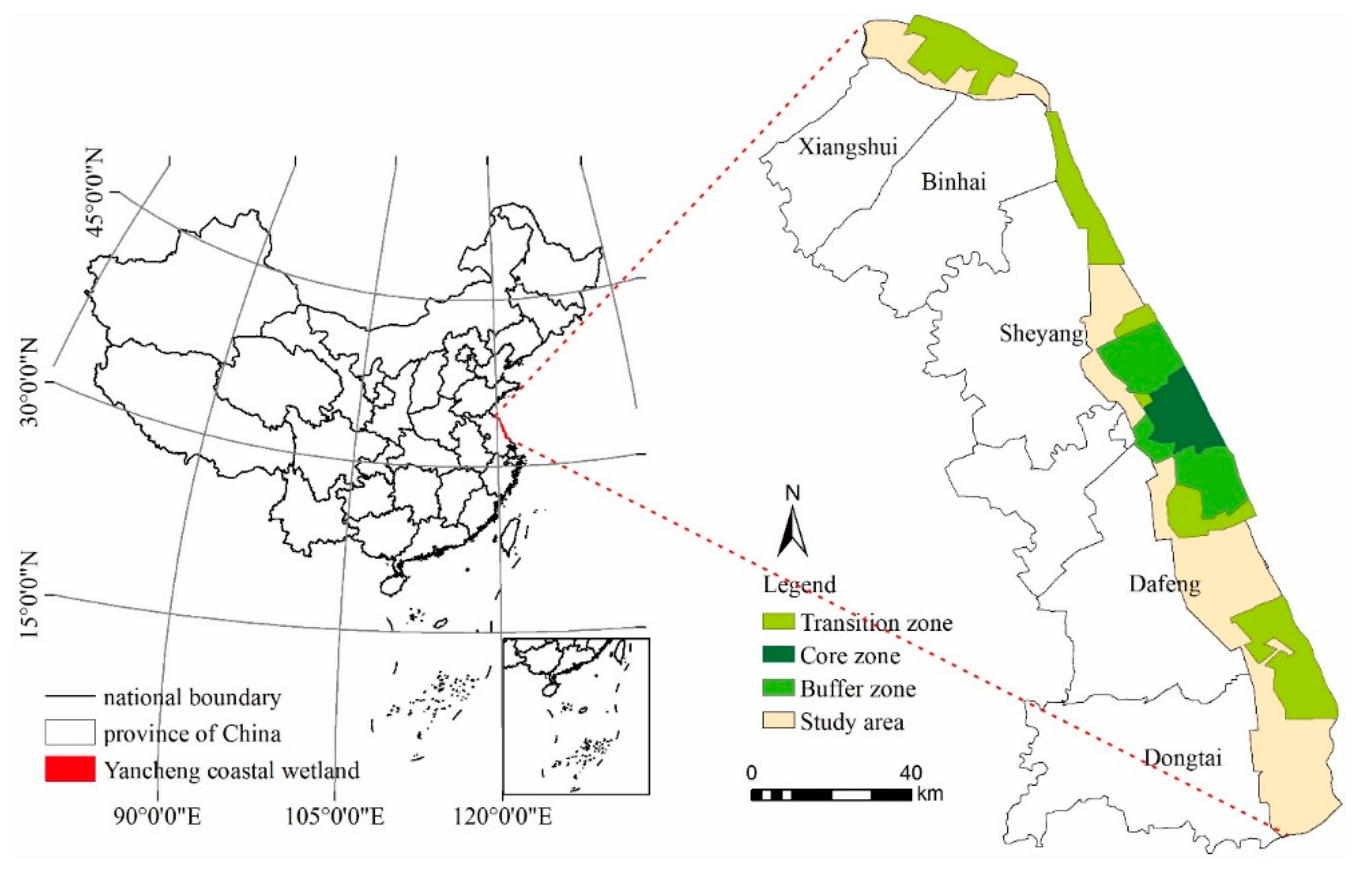
Figure 1. Geographical location of the study area.
Sustainability 13 00149 g001
Figure 2. Spatial distribution of landscapes in Yancheng coastal wetland.
Sustainability 13 00149 g002
Figure 3. Multi-scenario landscape simulation and ecological risk assessment framework.
Sustainability 13 00149 g003
Figure 4. Spatial distribution of landscape types simulated under multi-scenario during 2021–2025.
Sustainability 13 00149 g004
Figure 5. Spatial distribution of major conversion types. Note: OTT: other transfer types; TF: Tidal flat; AQ: aquafarm; PA: Phragmites australis; FL: farmland; SA: Spartina alterniflora; SS: Suaeda salsa; DP: dry pond; seawater: SW; SP: Salt pan.
Sustainability 13 00149 g005
Figure 6. Spatial distribution of major transfer types under the multi-scenario landscape simulation. Note: OTT: other transfer types; TF: Tidal flat; AQ: aquafarm; PA: Phragmites australis; FL: farmland; SA: Spartina alterniflora; SS: Suaeda salsa; DP: dry pond; seawater: SW; SP: Salt pan.
Sustainability 13 00149 g006
Figure 7. Change characteristics of risk areas during 1991–2017.
Sustainability 13 00149 g007
Figure 8. Spatial change characteristics of ecological risk during 1991–2017.
Sustainability 13 00149 g008
Figure 9. Trends of risk area change in different scenarios during 2021–2025.
Sustainability 13 00149 g009
Figure 10. Spatial distribution of ecological risk under different landscape simulations.
Sustainability 13 00149 g010
Figure 11. Transfer rates of major ecological risk transfer directions during 1991–2017. Notes: EXL: extremely low; LOW: low; REL: relatively low; MED: medium, REH: relatively high; HIG: high; EXH: extremely high.
Sustainability 13 00149 g011
Figure 12. Transfer rates of major ecological risk transfer directions during 2017–2025. Notes: EXL: extremely low; LOW: low; REL: relatively low; MED: medium, REH: relatively high; HIG: high; EXH: extremely high.
Sustainability 13 00149 g012
Publisher’s Note: MDPI stays neutral with regard to jurisdictional claims in published maps and institutional affiliations.