Exploring the Spatial and Temporal Relationship between Air Quality and Urban Land-Use Patterns Based on an Integrated Method

Abstract

The deterioration of air quality in urban areas is often closely related to urbanization, as this has led to a significant increase in energy consumption and the massive emission of air pollutants, thereby exacerbating the current state of air pollution. However, the relationship between urban development and air quality is complex, thus making it difficult to be analyzed using traditional methods. In this paper, a framework integrating spatial analysis and statistical methods (based on 170 regression models) is developed to explore the spatial and temporal relationship between urban land use patterns and air quality, aiming to provide solid information for mitigation planning. The thresholds for the influence of urban patterns are examined using different buffer zones. In addition, the differences in the effects of various types of land use pattern on air quality were also explored. The results show that there were significant differences between 1999 and 2013 with regards to the correlations between land use patterns and air pollutant concentrations. Among all land uses, forest, water and built-up areas were proved to influence concentrations the most. It is suggested that the developed framework should be applied further in the real-world mitigation planning decision-making process

1. Introduction

The intensification of global urbanization has exacerbated the negative impact of various environmental factors in urban areas, thus threatening the sustainability of future urban development on multiple fronts. In order to ensure the sustainability of urban environments, the use of urban or environmental planning as tools to formulate countermeasures has become an issue of great concern among government agencies. Of the various natural and man-made hazards, air pollution has been increasingly regarded as an important topic of research because it exerts constant tangible and intangible effects on the physical and mental health of urban residents, thereby indirectly affecting the social and economic activities of urban areas. In recent years, countries around the world have gradually begun to examine the causes and negative effects of air pollution in urban areas from the perspectives of sustainable development and urban planning, as well as the possible adaptations and mitigations to address these issues. From this, we can see that air pollution has a considerable impact on the sustainable development of cities [1,2,3]. In addition, numerous studies have shown that air pollution has a significant impact on human health [4,5,6]. The most common air pollutants in cities include carbon dioxide (CO₂), carbon monoxide (CO), sulfur dioxide (SO₂), nitrogen oxides (NO_x), hydrocarbons (HC), suspended particulate matter (SPM, including PM10, PM2.5), heavy metals (HM), ozone (O₃), smog, and chlorofluorocarbons (CFC). For example, residents living near major traffic thoroughfares were subject to long-term exposure to traffic-related air pollutants, such as black smoke and NO₂, which lead to increased cardiopulmonary mortality [7].

The deterioration of air quality in urban areas is often closely related to urban development, public facilities, and traffic patterns. As urbanization has resulted in rapid population growth and increased economic activities, this has led to changes in land use and transportation modes, which have also led to a significant increase in energy consumption and the massive emission of air pollutants, thereby exacerbating the current state of air pollution [6,8,9]. The appropriate implementation of urban planning also has a significant impact on the air quality of the same areas and the possible extent of air quality deterioration [10]. Therefore, this shows the importance of studying urban air quality from the perspective of urban planning. Past studies on urban development and air quality have found that urban building layouts, urban planning patterns, building height, and other factors can affect the air quality in urban environments, thereby influencing urban sustainability [11,12]. The main factor is the different patterns of urban planning or development, which can affect building height, spacing between adjacent buildings, and building layout in cities, thereby influencing the dispersion and accumulation of different air pollution sources in different ventilation environments. On the other hand, urban spatial patterns and land use types can also have a relatively significant impact. Therefore, by adopting reasonable planning methods, it should be possible to create the appropriate urban wind environment and microclimate, which will improve the air quality of urban areas.

Relevant studies have explored the association between the degree of urbanization and air pollution. For example, Fang et al. [9] examined the comprehensive impact and spatial variations of urbanization in China on air quality, measuring air quality by using the Air Quality Index (AQI). Other studies have also directly examined the relationship between land use and air pollution. For instance, Borrego et al. [2] showed that cities with mixed land use provided better air quality compared to cities with low population density and disperse land use. Tang and Wang [13] demonstrated that urban forms had a significant impact on traffic-induced noise and air pollution. More specifically, historical areas with narrower roads, complex road networks, and higher density intersections had lower noise pollution but greater street canyon effects, which led to higher CO concentrations. Beelen et al. [14] verified the relationship between traffic and urban land with NO₂ and NO_x, showing that the concentrations of the above air pollutants were higher in areas closer to major roads or cities. Bereitschaft and Debbage [15] showed that metropolitan areas with sprawling urban forms had higher air pollution and CO₂ emissions after controlling for population, land area, and climate. Their study also pointed out that green infrastructure could help to improve air quality.

Based on the aforementioned studies, we can see that research on urban land use and air quality is becoming increasingly important. Nevertheless, it is not only the types of land use, but also the patterns and structures of land use that can have an impact on urban functions and air pollution [2,6,13,16]. More specifically, the impact of urban land use patterns on pollutant emissions can be explored through population density, emissions from motorized vehicles, and street layout among other factors [2,14,15]. Therefore, gaining a better understanding of the relationship between urban spatial patterns and air quality will help us to determine the most effective use of urban land that will enable the healthier development of cities [6,17]. Liu and Shen [18] focused on the pattern in changes in green spaces within the Taipei Metropolitan area in order to investigate their impact on air pollution. The study’s findings indicated that green spaces were negatively correlated with air pollution and that greater spatial aggregation led to more centralized green spaces, which facilitated the reduction of air pollution and urban temperatures. Xie and Wu [16] studied the effects of land use patterns on PM2.5 in Shenzhen, and they found that vegetation could effectively reduce the concentration of PM2.5. The study also pointed out that the percentage of land (PLAND) and edge density (ED) had significant effects on PM2.5, such that the larger the area of vegetation, the lower the concentration of PM2.5. In terms of the overall landscape, the more fragmented the land, the worse it was at reducing the concentration of particulate matter. Weber et al. [5] showed that urban land use patterns could predict the level of acoustic noise and the concentration of particulate matter (PM10). In particular, ED, patch density (PD), area-weighted mean patch fractal dimension (AWMPFD), Shannon’s diversity index (SHDI), and Shannon’s evenness index (SHEI) of residential areas were highly correlated with acoustic noise level and PM10 concentration. Furthermore, higher ED and PD of built-up areas led to higher acoustic noise levels and PM10 concentration. Detailed definition of the landscape metrics mentioned above could be found in [5,16,19].

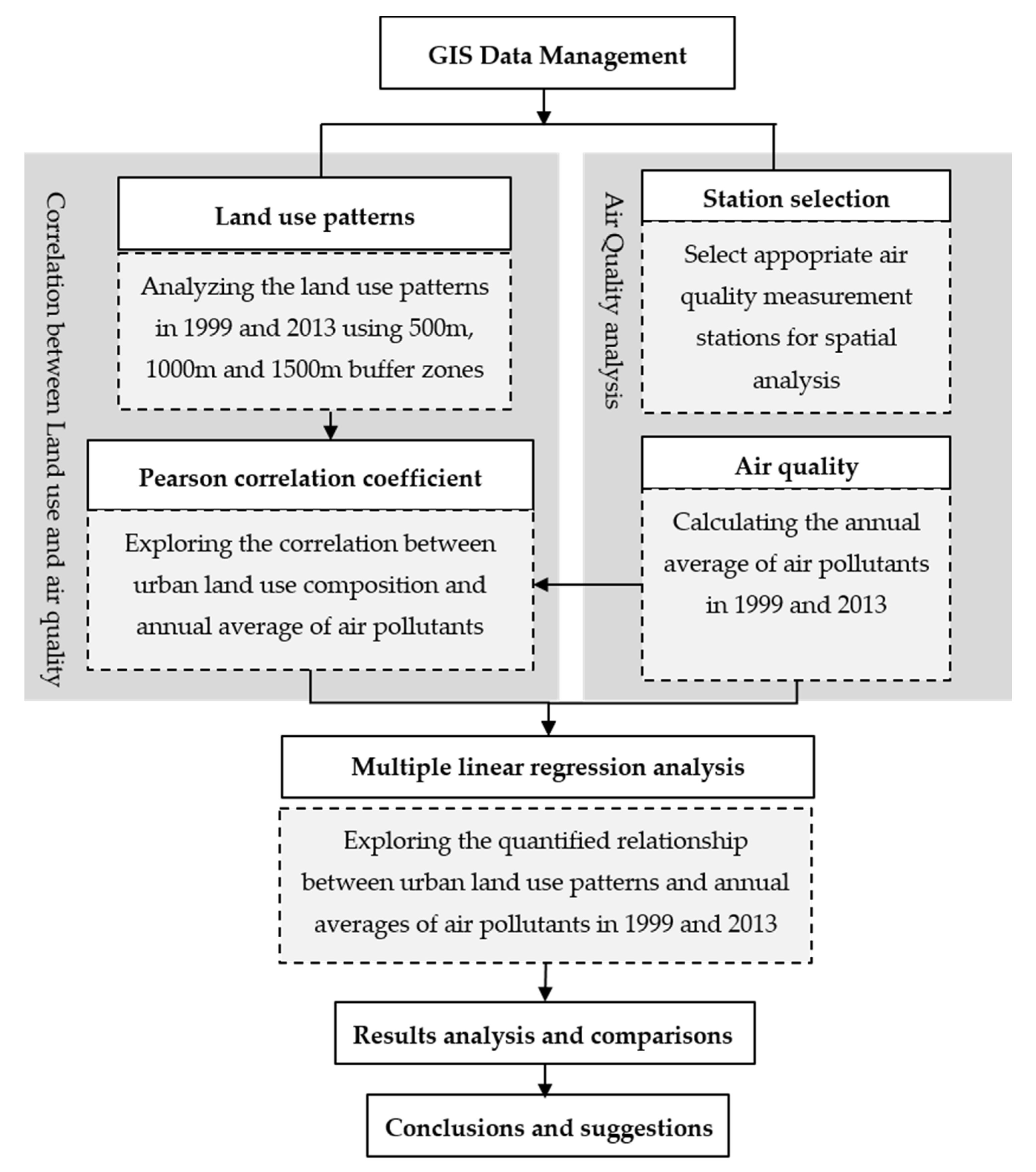
In order to gain a deeper understanding of the effectiveness of strategies for improving future urban air quality, integrated research methods, including the quantification of urban spatial patterns and structures and the correlation analysis between air quality and urban form, should be carried out. In view of this, a spatiotemporal analytical framework is constructed in this study, which involves first a correlation analysis between land use type indicators and air quality indicators at different spatial distances, followed by multiple sets of regression analysis based on data from different years. Our aim is to clearly quantify the correlation between different land use patterns and air quality in cities, which can serve as a reference for the future formulation of mitigation and adaptation planning strategies. This study will calculate the land use patterns within the different buffer radii of air quality monitoring stations and will explore the association between urban land use patterns and air quality using statistical analysis in order to serve as an important reference for the formulation of adaptation strategies related to air quality, which can benefit future land use planning. This proposed framework aims to provide useful information for public sectors when developing air-quality management strategies in the urban areas.

2. Materials and Methods

2.1. Study Area

Since urban development is closely related to air pollution, consideration was given to areas in Taiwan with a high degree of urbanization. Hence, the Northern Taiwan Air Quality Region (Taipei City, Keelung City, New Taipei City, Taoyuan City) and Taichung City were selected as the study area. A total of 30 EPA air quality monitoring stations were included in the study area in order to explore the correlation between urban land use patterns and air quality (Figure 1).

2.2. Research Framework

The research study was divided into two parts (see Figure 2). The first part involved the measurement of air pollutant concentrations, in which the annual averages of concentrations in 1999 and 2013 were calculated based on daily data. The second part involved analyzing spatial land use patterns within buffer distances (500 m, 1000 m, and 1500 m) from the 30 monitoring stations in the study area. Land use profiles and patterns were calculated and correlation coefficients were obtained to examine the correlation between land use composition and air pollution. Finally, we examined the association between the two parts above, using multiple regression analysis to explore the correlation between land use patterns and air quality. We then present an analysis of the results and a discussion, followed by a summary of the conclusions and recommendations of this study.

2.3. Data for Air Quality Measurement

According to the Air Quality Monitoring Report published by the Environmental Protection Administration (EPA) [20], Taiwan began establishing air quality monitoring stations in 1980, and a total of 76 stations were established by the end of 2019. The monitored pollutants included PM10 (suspended particulate matter below 10 um in diameter), SO₂, nitric oxide (NO), NO₂, NO_x, CO, O₃, and hydrocarbons (methane and non-methane hydrocarbons). Auxiliary meteorological parameters such as wind direction, wind speed, air pressure, temperature, and rainfall were also available. In addition, since August 2005, all monitoring stations were equipped with automatic monitors for fine SPM 2.5μm in diameter (PM2.5). Taiwan is now converting from the existing two-item test, the Pollutant Standards Index (PSI) and PM2.5, into a single index—the AQI. The AQI uses monitoring data to convert the daily concentrations of CO, O₃, SO₂, PM2.5, PM10, and NO₂, as well as their impact on human health, into sub-indices for different pollutants. Then, the maximum value of each sub-index for that day is set as the AQI of the day for that station.

This study selected the pollutants PM10, SO₂, NO₂, CO, and O₃ for the calculation of pollutant concentrations. Annual averages of the above air pollutants in 1999 and 2013 were calculated for the 30 EPA air quality monitoring stations. These averages allowed us to examine the status and variations in air quality during these 14 years and served as a basis for subsequent analyses of air pollutants. According to the statistical description of monitoring stations provided by the EPA, the units of measurement were defined as follows:

• Hourly average: This refers to the arithmetic mean of all values measured within one hour. In order to ensure the representativeness of the data, an hourly average is only considered valid when the total number of samples analyzed per hour is ≥ 75% for the automatic monitors of each pollutant in the Air Quality Monitoring Network.
• Daily average: This refers to the arithmetic mean of all hourly averages within one day. A daily average is only considered valid when the number of valid hours within a day is ≥16 h.
• Annual average: This refers to the arithmetic mean of all daily averages within the year. The annual average is only considered valid when the number of valid hours in a year is ≥6000 h.

2.4. Land Use Data and Landscape Analysis

Detailed investigation data is one of the key factors that determine the accuracy of the landscape analysis. Thus, the land use surveys conducted in 1999 and 2013 by the National Land Surveying and Mapping Center of the Ministry of the Interior were used as the basic data set in this study. The data were produced based on integrating remote-sensing techniques and ground survey methods. Using the geographic information system (GIS) ArcMap 10.3, the layer data were defined as the classifications in the first level of the land use classification system, namely, (1) agriculture (2) forest (3) transportation (4) water (5) building (6) public facility (7) recreation (8) mineral, and (9) others. Considering the effects of coverage of urbanized areas on air quality measurement and the distance influence of such effect, the land use types and patterns were calculated for the buffer zones of 500 m, 1000 m, and 1500 m around the 30 monitoring stations in the study area, as shown in Figure 3. The threshold distances were determined considering the spatial resolution and scale of the neighborhood according to our land use investigation data (starting with 500 m and increasing by 500 m to account for uncertainty).

In landscape ecology, landscape metrics provide the composition and configuration of the relevant landscape and describes the spatial structure of individual patches, specific classes of patches, and entire landscapes [21] (Gustafson, 1998). Landscape spatial patterns can be analyzed on three scales: patch-level index describing individual patches, class-level index describing a patch type or class composed of several patches, and landscape-level index describing the entire landscape mosaic that includes several patch types [22] (Wu, 2003). In addition to being able to quantitatively describe and monitor the changes in landscape structure characteristics over time, it can also be used to identify the spatial gradients of ecological characteristics in the landscape [22] (Wu, 2003). The most commonly used analytical tool for landscape metrics is FRAGSTATS developed by McGarigal and Mark in 1995 under the commission of the US Department of Agriculture. The version used in this study is FRAGSTATS 4.2, which was combined with geographic information system (GIS) for the input, analysis, and simulation of spatial information, in addition to the calculation of the composition and spatial distribution patterns of the landscape structure in the study area.

In terms of examining the land use patterns, landscape metrics for the nine land use classifications were calculated in order to quantify the area ratio (composition) and spatial arrangement (configuration) of each land use type at the landscape level. Regarding the landscape metrics used in relevant studies in Taiwan and abroad, PLAND, PD, largest patch index (LPI), total edge (TE), ED, mean patch area (AREA_MN), aggregation index (AI), and area-weighted mean patch radius of gyration (GYRATE_AM) were selected in this study to quantify landscape patterns [23] (McGarigal, 2015).

3. Results

3.1. Effects of Buffer Zones on Correlation

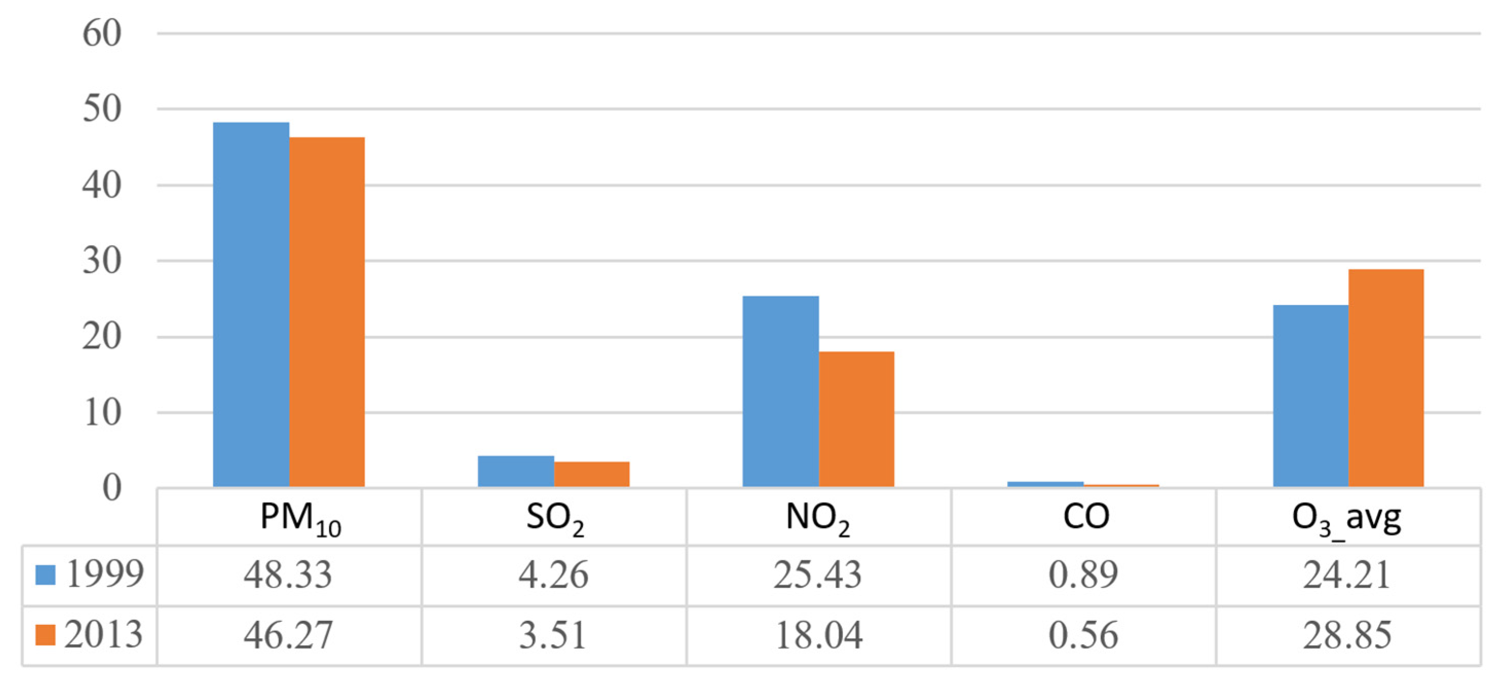
Based on the statistical description of the monitoring stations defined by the EPA, we calculated the annual averages for PM10, SO₂, NO₂, CO, and O₃ in 1999 and 2013 for the 30 stations. The annual averages of air pollutants in 1999 and 2013 were averaged across all monitoring stations, as shown in Figure 4, and the averages of the two years were compared. Overall, the averages of air pollutants in 1999 were all higher than those in 2013, except for O₃_avg in 1999, which was lower than that in 2013 (p value < 0.01). The exception for O₃ reflected the complex production and depletion processes of O₃, since it can be either depleted with NO producing NO₂, or can be produced by photochemistry at elevated temperature and volatile organic compounds. Therefore, the lower level of O₃ might result from a higher N2 level in 2013.

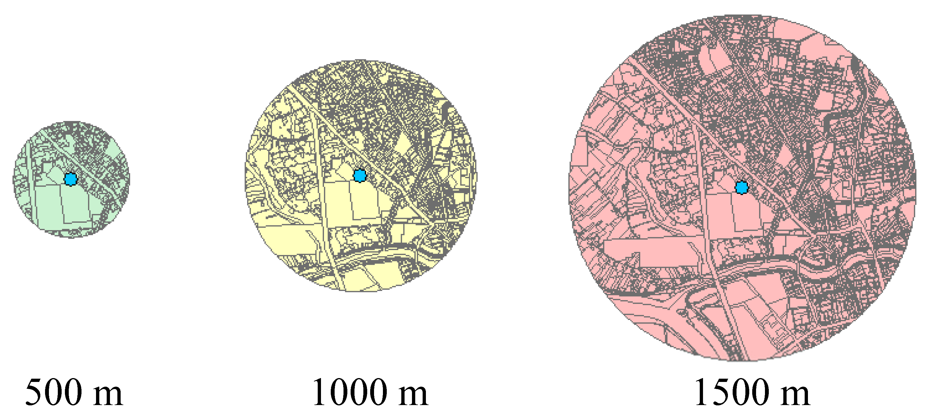
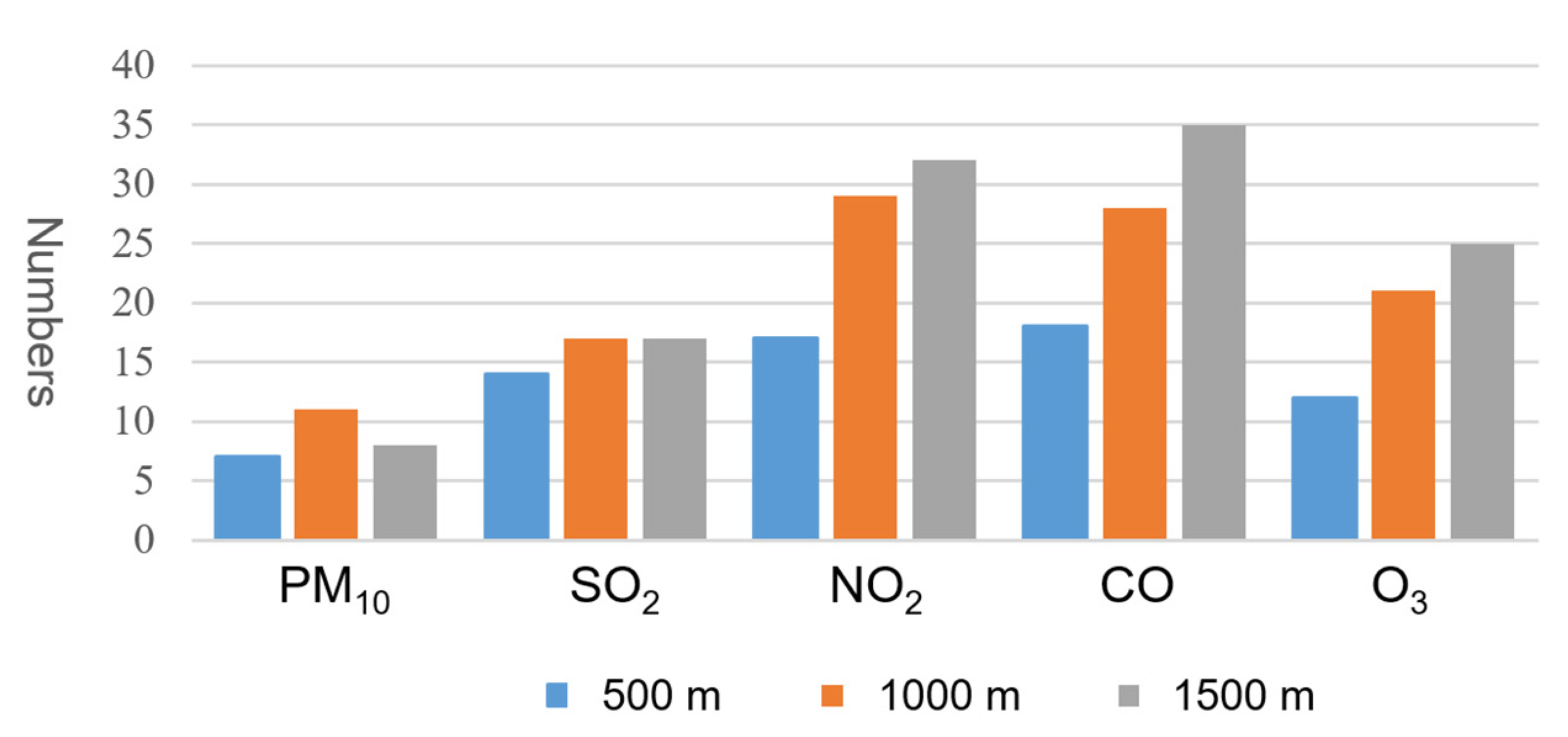
This study first employed the Pearson correlation coefficient to conduct a preliminary investigation on the correlation between air pollutant concentrations and land use patterns in different buffer zones. Specifically, the correlations between land use patterns and air pollution concentrations within the distances of 500 m, 1000 m, and 1500 m revealed the following: when exploring whether the correlation coefficients were at a moderate level or above (positive correlation > 0.3, negative correlation < −0.3 [24], p value < 0.01), it is found that within the 1500 m range, many of the correlations between land use patterns and air pollutant concentrations were relatively high (see Figure 5). Therefore, a buffer zone of 1500 m around the 30 monitoring stations in the study area will be used in the subsequent sections to explore the association between land use patterns and air pollutant concentrations in 1999 and 2013.

3.2. Change in Urban Land Use Patterns

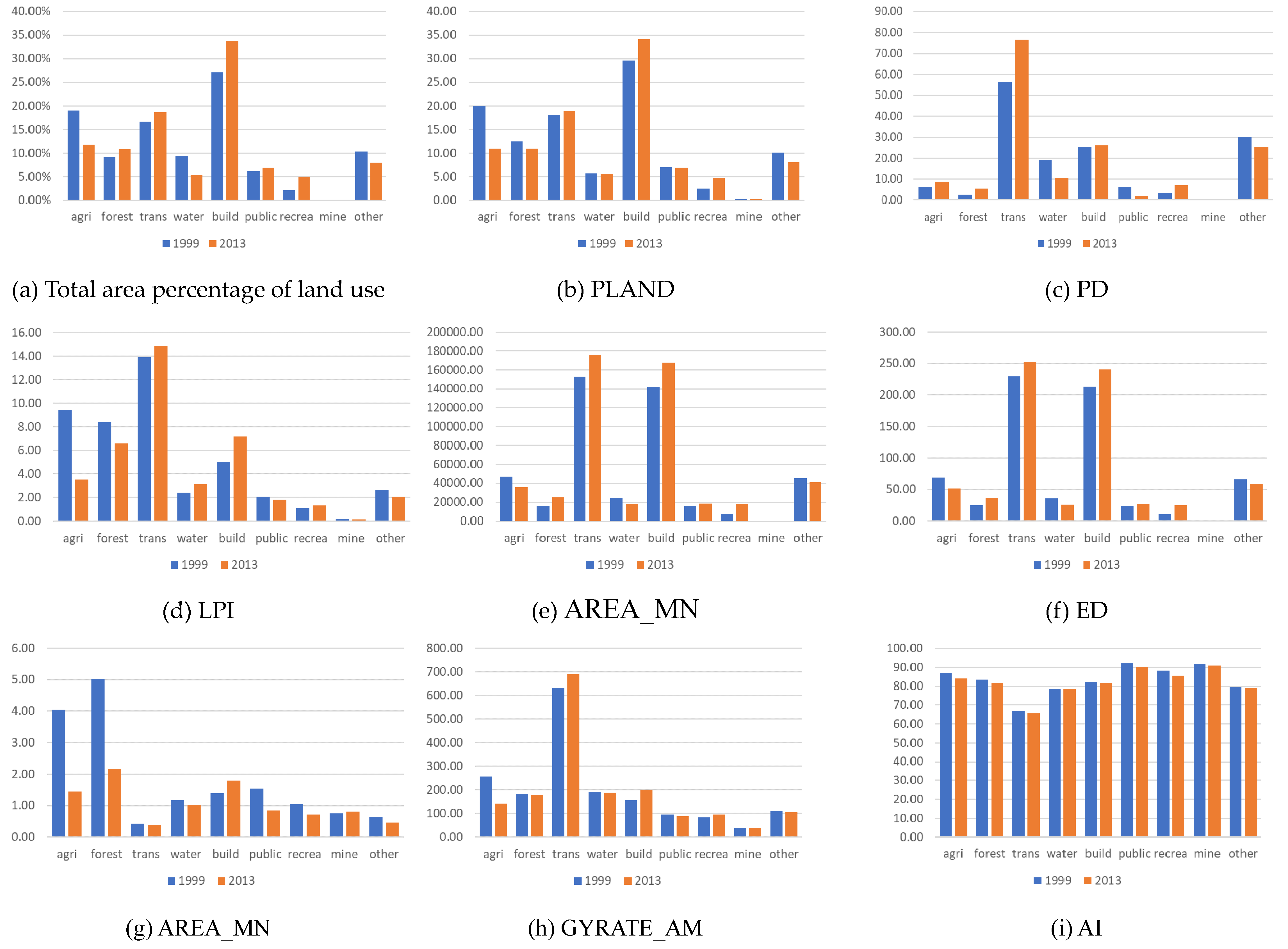
Based on a buffer distance of 1500 m around the 30 monitoring stations in the study area, we calculated the profiles and patterns of land use types in 1999 and 2013. Subsequent analysis was based on the nine classifications of the first level of the land use classification system, which includes agriculture, forest, transportation, water, building, public facility, recreation, mineral, and others. Among the overall land use types for the two years, buildings accounted for the largest area in both years and the largest increase in area, increasing by about 6.57%; agriculture accounted for the greatest reduction in area, decreasing by about 7.32%; water, mineral, and others showed a decrease in area; and forest, transportation, public facility, and recreation increased in area (see Figure 6a and

Table 1. The area of each land use type in 1999 and 2013.

Land Use Type	1999		2013		Percentage of change (%)
	$\mathbf{Area}\left(\mathbf{k}{\mathbf{m}}^2\right)$	Percentage (%)	$\mathbf{Area}\left(\mathbf{k}{\mathbf{m}}^2\right)$	Percentage (%)
Agriculture	37.15	19.01%	22.84	11.68%	−7.32%
Forest	17.87	9.14%	21.16	10.83%	1.69%
Transportation	32.62	16.69%	36.40	18.62%	1.93%
Water	18.37	9.40%	10.57	5.41%	−3.99%
Building	53.04	27.13%	65.88	33.71%	6.57%
Public Facility	11.89	6.09%	13.39	6.85%	0.77%
Recreation	4.11	2.10%	9.66	4.94%	2.84%
Mineral	0.23	0.12%	0.21	0.11%	−0.01%
others	20.17	10.32%	15.34	7.85%	−2.47%
total	195.45	100.00%	195.45	100.00%

).

Following which, the study area covering a buffer zone of 1500 m around the 30 monitoring stations was segmented into 30 sample plots, and FRAGSTAT 4.2 was used to calculate the eight landscape metrics of the nine land use types in each sample plot for the two years. Firstly, in terms of PLAND (see Figure 6b), building had the largest average in both years and the greatest magnitude of increase, with its area rising by 4.56%. Agriculture, forest, and others all showed a decreasing trend across the two years, with agriculture showing the greatest reduction of 9.00%. The aggregation index (AI) indicates that (Figure 6i) all nine land use types showed decreasing trends, among which the decrease in the AI of agriculture was the largest at 3.23%; that of forest, public facility, and recreation were similar at 2.05%, 2.28%, and 2.69%, respectively; while the changes in other types were not significant. The area-weighted mean patch radius of gyration (GYRATE_AM) indicated that (Figure 6h) transportation and building both showed increasing trends, rising by 60.13 and 42.64, respectively, whereas that of agriculture showed the greatest reduction, decreasing by 115.34. The largest patch index (LPI) indicated that the LPI of transportation, which increased by 1.00% and showed greater patch aggregation, was the highest for both years (Figure 6d) and that of agriculture and forest decreased by 5.92% and 1.79%, respectively, and showed decreased aggregation. Fragmentation was described using PD, AREA_MN, AREA_MN, and ED (see Figure 6c,g,e,f), which indicated that forest and agriculture showed marked changes in fragmentation between the two years, of which agriculture showed a relatively distinct trend of increasing fragmentation.

3.3. Relationship between Land Use Patterns and Air Quality

The Pearson correlation coefficient was used to investigate the correlation between air pollutant concentrations and land use compositions within a buffer zone of 1500 m around the 30 monitoring stations. The correlation coefficients between PM10, SO₂, NO₂, CO, and O₃ concentrations with PLAND were analyzed for the nine land use types and considered whether the correlation coefficients were at or above a moderate level (positive correlation > 0.3, negative correlation < −0.3 [24], p value < 0.01) in order to facilitate subsequent analysis and discussion (

Table 2. The correlation coefficients between air pollutants and land use compositions.

Land use Types	PLAND of 1999					PLAND of 2013
	PM10	SO2	NO2	CO	O3.avg	PM10	SO2	NO2	CO	O3.avg
Agriculture	−0.0613	−0.041	−0.3851	−0.4256	0.0416	0.3383	0.3195	−0.3829	−0.3999	0.2944
Forest	−0.3937	−0.4669	−0.6271	−0.3313	0.8015	−0.5211	−0.3715	−0.6579	−0.4158	0.7057
Transportation	0.3225	0.3141	0.7726	0.5818	−0.6688	0.2656	0.1302	0.7828	0.5543	−0.7980
Water	−0.0401	−0.0869	0.1167	0.1089	−0.2587	−0.0216	−0.1435	0.2097	0.2704	−0.1372
Building	0.4650	0.4635	0.7956	0.6544	-0.6783	0.3916	0.2823	0.7172	0.5304	−0.6766
Public Facility	−0.0542	0.1512	0.3954	0.3211	−0.3398	0.1384	0.0839	0.4985	0.3026	−0.5562
Recreation	0.1844	0.0171	0.4006	0.3722	−0.2622	−0.1790	−0.2517	0.3824	0.3665	−0.4177
Mineral	−0.0855	−0.4327	−0.4610	−0.3565	0.1389	0.0212	−0.5555	-0.1115	−0.3519	0.0764
Others	0.0626	0.0486	−0.0124	−0.2221	−0.1860	−0.2187	−0.0388	-0.4562	−0.4301	0.3949

).

Based on the individual air pollutant concentrations, it is found that the annual average of PM10 was negatively correlated with forest components and positively correlated with building components. The annual average of SO₂ was negatively correlated with forest components and mineral components. The annual average of NO₂ was negatively correlated with agriculture and forest components, and positively correlated with transportation, building, public facility, and recreation components. The annual average of CO was negatively correlated with agriculture, forest, and mineral components, and positively correlated with transportation, building, public facility, and recreation components. The annual average of O₃ was positively correlated with forest components and negatively correlated with transportation, building, and public facility components. Among them, the annual averages of NO₂ and CO had the highest correlations with land use composition, whereas the correlations between other air pollutants and land use composition were relatively low.

In terms of land use types, agricultural and forested areas were negatively correlated with air pollutant concentrations, thus indicating that the greater these areas, the lower the pollutant concentrations. Transportation, building, public facility, and recreation were positively correlated with air pollutant concentrations, thus indicating that the greater these components, the higher the pollutant concentrations. Among them, forest had the highest correlation with air pollutant concentrations. To summarize the above, greater agricultural and forested area resulted in lower air pollutant concentrations, except for O₃ concentration, which increased; while greater transportation, building, public facility, and recreation components led to higher air pollutant concentrations, except for O₃ concentrations, which decreased. The reason why this reverse relationship between land uses and O₃ concentrations occurred might be because ozone is a secondary pollutant generated from chemical reactions of other compounds. This probably means that depletion was dominant process with the NO₂ concentrations increasing. The overall increase in O₃ suggests that increased volatile organic compounds and elevated temperatures in summer contribute to ozone production more significantly than the localized decrease by increasing transportation. Overall, it could be inferred that manmade infrastructure and buildings might be the influential factors when considering mitigating air pollution in urban areas, indicating the importance of proper spatial planning in the region.

Multiple regression analysis was then employed to examine the association between air pollutants and the land use patterns. The dependent variable y is the annual average of the air pollutants, and the independent variable x is the landscape metrics of different land uses. This was followed by the analysis of the correlation between air pollutants and the same pattern of different land uses in 1999 and 2013. In the following sections, the analysis will be divided into four parts according to the target year and the influencing factors. A total number of 170 regression models were conducted to analyze the complex relationship between land use pattern and urban air quality. All models passed multicollinearity tests (VIF < 3) and normality tests for residuals (K-S tests with P = 0.01). As shown in

Table 3. Dependent and independent variables for each regression group.

Regression Group	Impact of spatial pattern (1999)	Impact of spatial pattern (2013)	Impact of land use type (1999)	Impact of land use type (2013)
Dependent variables (x)	Landscape metrics (one-at-a-time) for the nine land use types surrounding station i in 1999 in a model	Landscape metrics (one-at-a-time) for the nine land use types surrounding station i in 2013 in a model	Eight landscape metrics for one land use type surrounding station i in 1999 in a model.	Eight landscape metrics for one land use type surrounding station i in 2013 in a model.
Independent variables (y)	Annual average of the five air pollutants at station i.	Annual average of the five air pollutants at station i.	Annual average of the five air pollutants at station i.	Annual average of the five air pollutants at station i.
Total number of regression models conducted	40	40	45	45

, the classification of regression groups would help investigate into the differences between the effects of land use types and the overall spatial pattern of land uses. The results are summarized in the following section.

3.3.1. Spatial Relationship between Land Use Types and Air Quality in 1999

In this part of the analysis, 80 regression models (40 for each year) were performed to explore the relationship between a certain metric of different land uses and air pollution concentrations, to understand what might be the most influential metrics. The level of significance was set to be 0.05. After considering whether the regression models reached the significance level (p < 0.05), it is found that the regression models between CO and the PD, ED, AREA_MN, and GYRATE_AM of each land use type all reached the significance level. In addition, the regression models between NO₂ and the PLAND, PD, LPI, TE, ED, AREA_MN, and GYRATE_AM of each land use type all reached the significance level. The regression models between O₃ and PLAND, PD, TE, ED, AREA_MN, and GYRATE_AM all reached the significance level. The regression models between PM10 and LPI, TE, ED, AREA_MN, GYRATE_AM, and AI all reached the significance level.

Following this, t-tests were performed to determine whether the individual independent and dependent variables reached the significance level (p < 0.05). Based on the data, the AREA_MN and GYRATE_AM of each land use type showed greater correlation with air pollutant concentrations, both reaching significance for CO, NO₂, O₃, and PM10. A summary of this part of the regression model results could be found in

Table 4. Summary of the regression model results in 1999 (40 models).

Air Pollution Type	Number of Models Reached Significance Level (out of the Eight Models)	Influential Landscape Metrics	R2 Range of the Significant Models
PM10	6	PLAND, LPI, TE, ED, AREA_MN, GYRATE_AM, AI	0.32–0.67
CO	4	TE, ED, AREA_MN, GYRATE_AM	0.31–0.48
NO2	7	PLAND, LPI, TE, ED, AREA_MN	0.47–0.54
O3	6	PLAND, TE, ED, AREA_MN, GYRATE_AM	0.45–0.53
SO2	2	AREA_MN, GYRATE_AM	0.24–0.33

. It can be seen that NO₂ has the highest number of models that reached significance level. This indicated that there are more landscape metrics proved to be influential on the concentration of NO₂ than others. Overall, the R square level (ranging from 0.24 to 0.67) indicated that land use metrics do explain the variation of the air pollution concentrations to a certain level. Although it also suggested that there are still other factors that might also influence

In terms of land use types, building land use patterns had marked effects on air pollutant concentrations. Specifically, the increase in building in PLAND, LPI, TE, and ED led to the increase in the annual averages of PM10 and NO₂; the increase in building in AREA_MN led to the increase in the annual averages of PM10 and NO₂ and the decrease in the annual average of O₃; and the increase in building in GYRATE_AM led to the increase in the annual average of PM10. On the other hand, forest land use patterns also had marked effects on air pollutant concentrations. Specifically, the increase in forest in TE and ED led to the decrease in the annual averages of PM10 and NO₂, while the increase in forest in AREA_MN and GYRATE_AM led to the decrease in the annual averages of CO, NO₂, and PM10 and the increase in the annual average of O₃. The increase in mineral use in GYRATE_AM also led to the decrease in the annual averages of CO, NO₂, and PM10, as well as the increase in the annual average of O₃. A summary of the analysis can be found in

Table 5. Summary of analysis of influence of land-use pattern on air pollution in 1999.

Land use Type	Air Pollution Concentrations Influenced Significantly	R2 Range of the Significant Models
Forest	SO2, PM10	0.36–0.42
Transportation	CO, NO2, O3, PM10	0.32–0.69
Water	CO, NO2, O3, SO2, PM10	0.31–0.55
Building	CO, NO2, O3, SO2, PM10	0.37–0.65
Public facility	NO2	0.28
Others	SO2	0.39

. There are six out of nine land use types that are proven to be related to the concentration of air pollutants, including forest, transportation, water, building, public facility and others. As shown in

Table 6. Summary of the regression model results in 2013 (40 models).

	Number of Models Reached Significance level (out of the Eight Models for Each)	Influential Landscape Metrics	R2 Range of the Significant Models
PM10	6	LPI, TE, ED, AREA_MN, GYRATE_AM, AI	0.42–0.73
CO	7	PLAND, TE, ED, AREA_MN, GYRATE_AM	0.31–0.48
NO2	8	LPI, TE, ED, AREA_MN	0.47–0.54
O3	6	PLAND, TE, ED, AREA_MN, GYRATE_AM	0.45–0.53
SO2	2	AREA_MN, GYRATE_AM	0.24–0.33

, different land uses have different impacts on air pollution concentrations. Among all pollutants, PM10, NO₂, and SO₂ are associated with at least four types of land use, suggesting the potential of mitigating such concentrations via proper spatial planning.

3.3.2. Spatial Relationship between Land Use Types and Air Quality in 2013

After considering whether the regression models reached the significance level (p < 0.05), we found that the regression models between CO and the PLAND, TE, ED, AREA_MN, GYRATE_AM, and AI of each land use type all reached the significance level. The regression models between NO₂ and the PLAND, PD, LPI, TE, ED, AREA_MN, GYRATE_AM, and AI of each land use type all reached the significance level. The regression models between O₃ and PLAND, PD, LPI, AREA_MN, GYRATE_AM, and AI all reached the significance level. SO₂ did not reach the significance level for any of the land use patterns. The regression models between PM10 and PLAND, LPI, TE, AREA_MN, GYRATE_AM, and AI all reached the significance level. The remaining regression models did not reach the significance level. A summary of this analysis can be seen in Table 6. It is found that the numbers of models that reached the significance level for PM10 and CO are higher than that in 1999, indicating that the influence of land use pattern on the two pollutants became more obvious. In addition, R square in general increased from 1999 to 2013, suggesting that the explanatory power of land use pattern for air pollutant concentrations became higher. This might be related to the denser distribution of built-up areas during the process of urbanization in the region.

The data revealed that in terms of land use types, building land use patterns had limited effects on air pollutant concentrations. Only forest land use patterns had marked effects on air pollutant concentrations. Specifically, the increase in forest in PD led to the decrease in the annual averages of NO₂, the increase in forest in TE and ED led to the decrease in the annual averages of PM10 and NO₂, the increase in forest in AREA_MN and GYRATE_AM led to the decrease in the annual averages of PM10 and NO₂. On the other hand, agricultural land use patterns also had marked effects on air pollutant concentrations. Specifically, the increase in agriculture in AREA_MN and GYRATE_AM led to the decrease in the annual average of NO₂, and the increase in agriculture in AI led to the decrease in the annual average of CO and the increase in the annual average of O₃. Water use patterns had an increased impact on air pollutant concentrations, whereby the increase in water in AREA_MN led to the increase in the annual averages of CO and NO₂ and the decrease in the annual average of O₃. Finally, the increase in the PLAND and AI of other land use types led to the decrease in the annual averages of CO and NO₂.

A short summary of the analysis can be found in

Table 7. Summary of analysis of influence of land-use pattern on air pollution in 2013.

Land use Type	Air Pollution Concentrations Influenced Significantly	R2 Range of the Significant Models
Forest	NO2, PM10	0.4–0.52
Transportation	CO, NO2, O3, PM10	0.37–0.7
Water	CO, NO2, O3, SO2, PM10	0.33–0.58
Building	CO, NO2, O3, SO2, PM10	0.43–0.72
Public facility	NO2, O3	0.31–0.45
Others	O3, PM10	0.39

. It could be seen that in general, the R square became higher than that in 1999, suggesting that land use factors became more influential. This again suggests that urbanization played a role in enhancing the concentrations of air pollutants. In terms of the effects of different land use types, forest, building, transportation and water uses are all proved to be very influential. Comparing built-up areas and natural resources, it is found that transportation and building are two of the most influential land uses. This matched the assumption that the appropriate planning for both built-up areas (transportation, building, public facility) and natural resources (forest and water) is crucial.

3.3.3. Summary

In 1999, the AREA_MN and GYRATE_AM of all land uses had more correlations with air pollutant concentrations, indicating that both area and shape of the land uses are influential. Among them, building, transportation, water and forest land use patterns had higher correlations with air pollutant concentrations. Specifically, the increase in building in PLAND, LPI, TE, ED, AREA_MN, and GYRATE_AM led to the increase in the annual averages of PM10 and NO₂, while the increase in forest in TE, ED, AREA_MN, and GYRATE_AM led to the decrease in the annual averages of PM10 and NO₂. In 2013, among the correlations between the land use patterns and air pollutant concentrations, the impact of building land use patterns was also very influential, and the increase in forest in TE and GYRATE_AM led to the increase in the annual averages of PM10 and NO₂, and the decrease in forest in ED and AREA_MN led to the decrease in the annual average of NO₂. According to the results from the above analysis, it could be seen that the change in relationship between air quality and land us pattern is evident from 1999 to 2013. This suggests that when the public or private sectors make attempt to mitigate air pollution, it is therefore important to consider the spatial and temporal relationship between land use and air quality in order to receive better results.

4. Discussions

According to the results, we can conclude that forest, building, water and transportation land use patterns had relatively high correlations with the annual averages of NO₂ and PM10 for both years. This suggests that we should emphasize the importance of spatial planning of such uses on mitigating air pollution in the urban areas. The increase in forest connectivity led to the decrease in the annual averages of PM10 and NO₂, and the increase in forest area led to the decrease in the annual average of NO₂. Therefore, we can conclude that forest land use patterns were highly correlated with the annual averages of NO₂ and PM10 in both years, whereby the increase in both forest areas and aggregation could reduce the concentrations of air pollutants. This finding is consistent with the assumptions presented in relevant studies [25,26], in which forest land use is found to be very influential on air pollutants concentrations in many regions. We can also infer that the planting of trees to mitigate the impact of air pollution is likely to be a crucial part of future spatial planning and design. Built-up areas, especially building and transportation, are also found to be very influential on the concentrations of the air pollutants studied in this research. According to Wang et al. [19], the compactness and other spatial patterns factors of buildings would significantly influence wind environment in urban areas, and this could be one of the main causes for unevenly distributed air pollutants concentrations. Edussuriya et al. [27] also derived similar conclusions from simulations, indicating that various land-use patterns have different impacts on air quality. Currently, the results from this studies matched the research findings above, all indicating that it is of crucial importance to carefully consider the spatial allocation of both forests and built-up areas in order to manage air quality.

In terms of the relationship between landscape metrics and air quality, it is found that both shape-based and area-based metrics could have some impacts on the concentrations. It could be inferred that the directions of buildings and streets and types of spatial allocation of buildings make a difference because they influence the wind environment significantly. This matched the findings in [28]. In addition to the impacts of wind environment, emissions on roads could also influence air pollutants concentrations, interacting with local wind environment [29]. The amount of emissions on the road could be significantly influenced by the form of urban blocks. This again stresses the importance and necessity of including both area and shape metrics in the analysis to identify the influences more clearly. Of course, it is worth noting that the selection of landscape metrics could possibly influence the results to some extents. Although in this paper up to eight metrics (representing spatial patterns from different angles) were used to quantify land-use patterns, there might still be other metrics that could be possibly useful to understand the relationship between land use and air quality. As a result, it is suggested that more metrics could be used in future research, considering the local characteristics and data type, to gain a wider view on the complex interactions between the two.

5. Conclusions

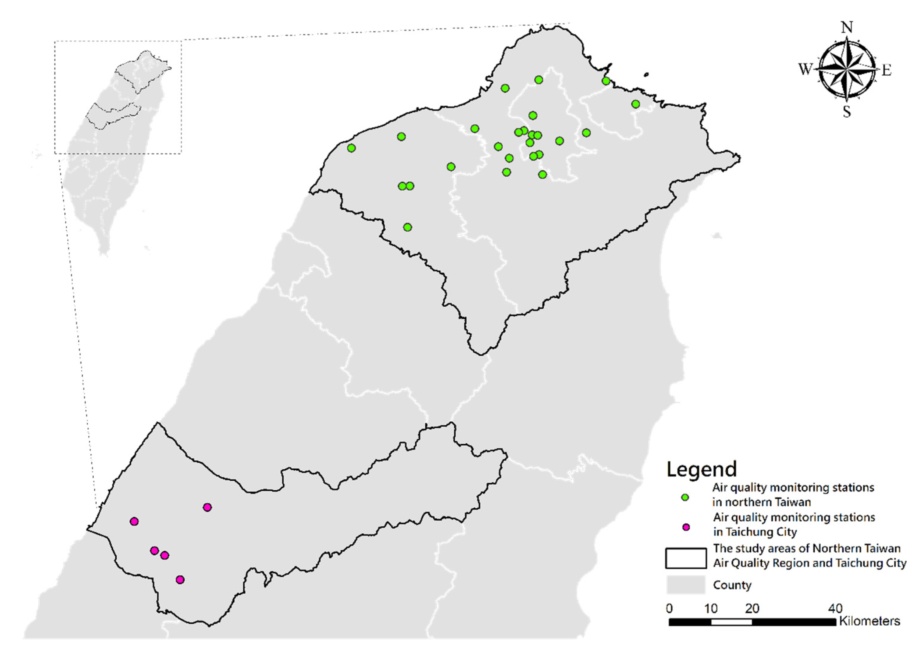
This study compared the pattern of changes in nine land use types between 1999 and 2013 for the Northern Taiwan Air Quality Region (Taipei City, Keelung City, New Taipei City, and Taoyuan City) and Taichung City, while also collecting and analyzing the annual averages of five air pollutants (PM10, SO₂, NO₂, CO, and O₃). It then examined the correlation between the patterns of the nine land use types and the annual averages of the air pollutants. With regard to the variation in air pollutant concentrations during the two years, the annual averages of all air pollutants decreased except for that of O₃, which increased. On the other hand, the change in the patterns of land used for agriculture and buildings were relatively large.

Landscape metrics were then used in this study to understand the changes in land use patterns during 1999 and 2013 in the study area, which included Taipei City, Keelung City, New Taipei City, Taoyuan City, and Taichung City. Overall, the building land use type had the highest total area and the greatest increase in area, while agricultural land use had the greatest reduction in area. Based on the 30 sample plots, building land use showed the highest area ratio with the greatest rate of increase and connectivity. Agricultural and forest land uses showed a decrease in area, substantial reductions in aggregation and connectivity, and increased fragmentation. Transportation land use showed increased land connectivity, while other land uses did not show significant changes.

The results of the correlation coefficients indicated that within a buffer zone of 1500 m around the 30 monitoring stations, air pollutant concentrations showed many correlations with the various land use patterns. Specifically, in terms of the correlation between air pollutant concentration and land use composition, the greater the agriculture and forest land use components within the 1500 m range, the lower the air pollutant concentration, and the higher the transportation, building, public facility, and recreation components, the higher the air pollutant concentration. This implies that the area of the built-up environment does indeed have a relatively significant impact on air pollution.

Multiple regression analysis indicated that there were significant differences between the two years with regards to the correlations between land use patterns and air pollutant concentrations. In 1999, building, transportation, water and forest land use patterns were highly correlated with air pollutant concentrations, such that the increase in building area and connectivity led to the increase in the annual averages of PM10 and NO₂, whereas the increase in forest area and connectivity led to the decrease in the annual averages of PM10 and NO₂. In 2013, built-up land use patterns had more impact, indicating that more emphasis should be put on proper planning for such land use.

Based on the current models, the relationship between land-use patterns and air pollutants concentrations is preliminarily revealed. Although some results suggested that more factors might need to be considered in future work, the current framework does provide more scientific foundation for planners and policy-makers when developing mitigation strategies. In addition, the quantitative results could help develop more sophisticated scenarios in the future work—to try to conduct CFD simulation models for further understanding of the consequences resulting from implementing different planning mitigation and adaptation strategies. Furthermore, as suggested earlier, there are many other factors in cities that might also influence air quality to various extents. For example, population density, vehicle emissions, and street arrangement will all lead to different forms and levels of air pollution. Of which, point source and nonpoint source forms of pollution can also affect the level of air pollution in cities. Furthermore, different climatic factors, such as temperature, rainfall conditions, humidity, and wind direction, may also affect the air flow or pollution conditions in different urban spaces. It is suggested that in future research, a comprehensive sensitivity analysis might be necessary to examine the actual influences of these factors on air pollutants concentrations. In terms of air quality data management, it is suggested that future studies should also consider applying geometric mean or median for yearly average calculation according to the actual statistical distributions of the data. Finally, disaster risks can also be influenced by hazard level, vulnerability, and exposure, this study recommends that in addition to examining the impact of spatial patterns on pollution, as mentioned above, future studies might also incorporate other socioeconomic, vulnerability, and exposure factors. It is suggested that a complete risk analysis of air pollution should be investigated as an important reference for the mitigation of urban air pollution using the relevant spatial planning methods in urban areas.