Article

The Linkages of Carbon Spot-Futures: Evidence from EU-ETS in the Third Phase

1
School of Economics and Management, Beihang University, Beijing 100191, China
2
College of Economics, Shenzhen University, Shenzhen 518061, China
3
School of Economics, Beijing Technology and Business University, Beijing 100048, China
*
Author to whom correspondence should be addressed.
Sustainability 2020, 12(6), 2517; https://doi.org/10.3390/su12062517
Submission received: 15 January 2020 / Revised: 27 February 2020 / Accepted: 20 March 2020 / Published: 23 March 2020

Abstract

:
Based on the prices selected from European Energy Exchange (EEX) from 2013 to 2018, we investigate the inter-correlation of carbon spot and futures markets. Specifically, we adopt the widely used DCC-GARCH model and VAR-BEKK-GARCH model to conduct a comprehensive analysis on the carbon market, i.e., the dynamic correlation and volatility spillover between carbon spot and carbon futures. Moreover, we develop a hedge strategy based on the VAR-BEKK-GARCH model and calculate the hedging effectiveness (HE) value to evaluate the strategy performance. The empirical results show that (i) during our sample period, carbon spot and futures markets are highly correlated, (ii) carbon spot overflows to the futures market and vice versa, and (iii) the HE value is equal to 0.9370, indicating a good performance for the hedging strategy. Then, we provide further discussion on the relationship between carbon spot and futures markets by replacing our dataset with the data of phase II. The results do not change our conclusions on the dynamic correlation and volatility spillover. However, the HE value of phase III is higher than that of phase II, which indicates that the carbon futures market of phase III is not only an available market to hedge risk from the contemporaneous carbon spot market but also has a better hedge effectiveness than phase II.

1. Introduction

Currently, one of the most thought-provoking issues globally is global warming, given its potential damage to agricultural production, industrial manufacture and human sustainable development [1,2]. Thus, the Kyoto Protocol established three mechanisms for climate change mitigation. Among all of the three mechanisms, emission trading is a unique way for carbon reduction, as it reduces carbon emissions through a market-based mechanism, which makes carbon reduction a market activity [3]. Based on the Kyoto Protocol, the European Union established the famous European Union Emission Trading Scheme (EU-ETS) in 2005. To date, the EU-ETS has been operating successfully for three phases. The first phase was from 2005 to 2007, the subsequent phase was from 2008 to 2012, and the third phase began in 2013 and will end in late 2020. Furthermore, the fourth phase of the scheme will launch in 2021, lasting for 10 years until late 2030 [4]. Due to the vast trading volume and drastic price changes, the EU-ETS has become the largest carbon trading market and is viewed as a common financial market for analyzing financial characteristics and portfolio management [5].
The carbon product traded in the EU-ETS is named the European Union allowance (EUA). Although the EU-ETS is a professional market for carbon trading, spot and futures trading are already proceeding as a common financial market. Accordingly, EUA carbon spot and futures prices should be correlated. The existing literature shows that the spot price can be forecasted without bias according to the corresponding futures price. A widely known reality in financial markets is that futures price reflects information of the spot price at the time when the futures contract has matured [6]. Thus, understanding the spot–futures price relationship helps market participants who are not fully hedged. Additionally, achieving a better understanding of the spot–futures relationship helps companies who are involved in the carbon market to manage their carbon assets and control risk. Moreover, the knowledge of interconnection and spillover are crucial issues to measure systemic risk across various markets [7]. To summarize, an in-depth study of the EU-ETS carbon spot and futures market is desirable.
This paper combines the study of energy economics and traditional finance, as we focus on a carbon trading market, analyzing the financial characteristics and their usefulness in portfolio management, i.e., dynamic correlation, volatility spillover and hedge strategy. The international EU-ETS has already continued for 14 years; however, little work has examined the spot-futures correlation inside the market, i.e., Arouri [6], Rittler [8], etc. Meanwhile, the previous literature mainly investigated the first two phases of the scheme, and only a few studies have centered on the current operating phase III [2]. Compared with the first two phases, however, the global emission reduction environment has changed considerably in phase III. For example, with ongoing development, China became the largest supplier [9] of Certified Emission Reduction (CER); meanwhile, both the EU-ETS and the carbon pilots of mainland China approved completing the compliance by partial CERs [10,11]. Thus, the cap-and-trade programs in China have affected EUA prices in the EU-ETS by the price of CERs, and Canada exited the Kyoto Protocol. Thus, phase III of the EU-ETS needs to be researched comprehensively to identify whether carbon strategies used in phase II are still suitable. In this paper, we further extend the current research by employing trading data in Phase III of the EU-ETS to fill the gap to some extent.
This paper makes the following contributions to the existing literature. We first adopt the dynamic correlation coefficient (DCC)-generalized autoregressive conditional heteroscedasticity (GARCH) model for summarizing the dynamics between carbon spot and futures in phase III of the EU-ETS, which is a reasonable extension of existing studies on the carbon allowance market for the first two phases. The empirical results remind the investors in the carbon market to avoid potential risk as carbon spot and futures are highly correlated. We then apply the vector autoregression (VAR)-Baba, Engle, Kraft, and Kroner, namely, the synthesized of acronym of four authors (BEKK) [12]-GARCH (VAR-BEKK-GARCH) model to study the volatility spillover between carbon spot and futures. To the best of our knowledge, it is the first application of the VAR-BEKK-GARCH model in the study of carbon spot–futures correlation during phase III of the EU-ETS. The empirical results show that carbon spot market overflows to carbon futures market, and vice versa, which deepens the understating of information spillover between carbon spot and futures prices and further benefits those investors who invest in both carbon spot and futures markets to hedge risk. Third, we develop a hedge strategy between carbon spot and futures, namely, a long position in the carbon spot and a short position of a certain hedge ratio in carbon futures, and we then calculate the HE value based on the results of the VAR-BEKK-GARCH model to illustrate our point on hedging risk. The result shows that the HE value is equal to 0.9370, which indicates that the hedged portfolio consisting of the carbon spot and carbon futures performs well. Finally, we conduct a further discussion on the linkage of the carbon spot and carbon futures by testing the trading data in phase II of the EU-ETS with the same methods. The results do not change our conclusions on the dynamic correlation and volatility spillover. However, the HE value calculated in phase II is equal to 0.8938, smaller than that in phase III. This interesting result for the HE value indicates that the carbon futures market in phase III of the EU-ETS can better hedge the risk from the carbon spot market when compared with phase II.
The remainder of this paper is organized as follows. Section 2 presents the literature review. Section 3 briefly introduces the Kyoto Protocol and the EU-ETS. Section 4 presents the methodologies used in this paper. Section 5 reports the empirical results. In Section 6, we provide further discussion on the linkage of carbon spot and futures in phase II and conduct a brief comparison with phase III. Section 7 concludes the paper.

2. Literature Review

Regarding the emerging carbon allowance markets, numerous studies have investigated the financial performance of carbon prices. For example, the empirical research of Paolella and Taschini [13] discovered the characteristic of asymmetries in the spot carbon price. A subsequent study performed by Benz and Trück [14] analyzed the dynamics of spot carbon prices. These researchers found strong evidence of nonlinear dynamics of spot carbon prices. In addition, the researchers also argued that the prices can be perfectly modeled by Markov-switching models. Benz and Hengelbrock [15] further demonstrated the price discovery process in the carbon market by selecting intraday price data from the ECX and Nord Pool exchange. These researchers argued that a more liquid market, i.e., the ECX exchange, is a leader to the less liquid market, i.e., the Nord Pool exchange. Based on an efficient market hypothesis, Daskalakis and Markellos [16] found that the three predominant EUA exchanges, i.e., ECX, Nord Pool, and Powernext, were not efficient during the initial phase of the EU-ETS from 2005 to 2007, which may be attributed to such factors as immaturity, banking and short-selling. Wei and Zhang [17,18] investigated the carbon price volatility in EU-ETS and China, respectively; the empirical results of both studies indicated the long-term memory in the carbon market. Based on the characteristics of carbon spot and futures, the research on the correlation between the two markets became a new research hotspot, as it is in the traditional financial markets, i.e., the oil market [19,20,21]. Milunovich and Joyeux [22] adopted novel econometric methods to investigate the efficiency of the EU-ETS and price discovery inside the scheme. The findings of these researchers indicate that there exists a bidirectional information transmission between carbon spot and futures markets in Phase I. Meanwhile, the empirical results further showed that over a long period of time, from December 2006 to December 2007, futures contract prices and the carbon spot were related. Moreover, the results also showed that the carbon futures market was a perfect market for risk mitigation from 2005 to 2007. An in-depth study still found evidence of the above standpoint [23]. However, Joyeux and Milunovich [24], as well as Chevalier’ [25] hold a different opinion; the two studies rejected the long-run relationship between carbon spot and futures prices in the first phase and the second phase of the EU-ETS, respectively. Furthermore, Chevalier [25] denied the bidirectional correlation between carbon spot and futures prices. Specifically, Chevalier [25] argued that the carbon spot price did not contribute to the price discovery in carbon futures market. Another in-depth study with intraday data conducted by Rittler [8] also supported the results that the relationship is not bidirectional. Joyeux and Milunovich [24] also focused on the issue of volatility transmission between carbon spot and futures markets. These researchers adopted a widely used BEKK-GARCH (1,1) model, and the result indicated the opposite position to that of Rittler [8]. Niblock and Harrison [26] selected several methods, e.g., unit root test and generalized impulse response functions, to analyze the correlation between carbon spot and futures markets during the first two phases. These researchers suggested that there existed dynamic linkages in the EUA carbon markets during the sample period. Based on the VAR and STR-EGARCH (Switching Transition Regression-Exponential GARCH) model, Mohamed, Fredj, and Duc [6] argued that the two markets are asymmetrically and nonlinearly linked. Stefan [3] comprehensively investigated the EUA spot and futures prices and pointed out that the carbon market changed from initial backwardation to contango. Gorenflo [27] used impulse response analysis and found that the EUA carbon futures market led the EUA carbon spot market in pricing discovery. In addition, Gorenflo [27] strongly argued that carbon futures contribute more to price discovery when compared with carbon spot. Meanwhile, he verified the cost-of-carry hypothesis that the futures price equals the spot price plus carrying cost in the carbon market for the first two phases of the EU-ETS. More recently, Balcilar [28] adopted an MS (Markov switching) -DCC-GARCH model for analyzing the potential linkages inside the carbon market, and the results strongly supported the time-varying cross-correlations and volatility spillover effects.
It is essential to note that existing studies mainly focused on the first two phases. Few studies paid attention to the operating third phase. Thus, there is a vacuum of current studies for the third phase regarding the linkages between carbon spot and futures. In this paper, we focus on the linkages during the third period to fill the gap.

3. Kyoto Protocol and EU-ETS

In December 1997, the Kyoto Protocol reached an agreement in Kyoto [2,29]. The Kyoto Protocol is an additional term of the United Nations Framework Convention on Climate Change (UNFCCC). The Kyoto Protocol is an international guideline of greenhouse gas emissions reduction for coping with the inevitable global warming after industrialization. However, the Kyoto Protocol is more binding compared with the UNFCCC. According to the protocol, the involved countries should control emissions of several greenhouse gases, e.g., carbon dioxide and sulfur hexafluoride [4]. As abatement technology varies across countries, not all countries can complete the tasks regulated by the protocol. Therefore, the protocol allows the related countries to conduct emission trading. Specifically, countries with excess emission allowances can sell their allowances to the countries with insufficient allowances [30]. According to mechanisms regulated by the Kyoto Protocol, i.e., emission trading, the European Union (EU) in 2005 made a far-reaching attempt to lead global emission reduction by establishing the well-known European Union Emission Trading Scheme (EU-ETS). Currently, the EU-ETS accounts for over seventy-five percent of carbon trading volume globally [6]. As the leader of global carbon reduction, the EU also approves the scheme to be linked with other countries’ carbon trading markets [31].
One of the foundations of the EU-ETS is called “cap-and-trade.” The total amount of greenhouse gases that can be emitted under the EU-ETS is called the “cap,” while “trade” means that the emitters can trade their allowances. The cap reduces year by year in order to meet the requirements of carbon reduction [32]. Within the cap, participants can trade their allowances with others if necessary. After one company obtains the allowances, the company should hold enough allowances to cover its emissions during the year [33]. Otherwise, the company will be fined heavily by the government. If one company has additional allowances, it can store them for the futures or sell them to the companies without sufficient allowances for profits. Thus, emission trading accomplishes maximized emission reduction with minimized cost.

4. Data and Methodology

4.1. Data

In this paper, we collect our dataset for EUA carbon spot and futures prices from the European Energy Exchange (EEX) during the period from 1 January 2013 to 26 December 2018. As there are several futures contracts traded in the time period, we select the continuous monthly contracts composed of the contracts of the largest open interest in each month to represent the carbon futures price in phase III of the EU-ETS. The price trend of the EEX EUA spot and futures is depicted in the following Figure 1.
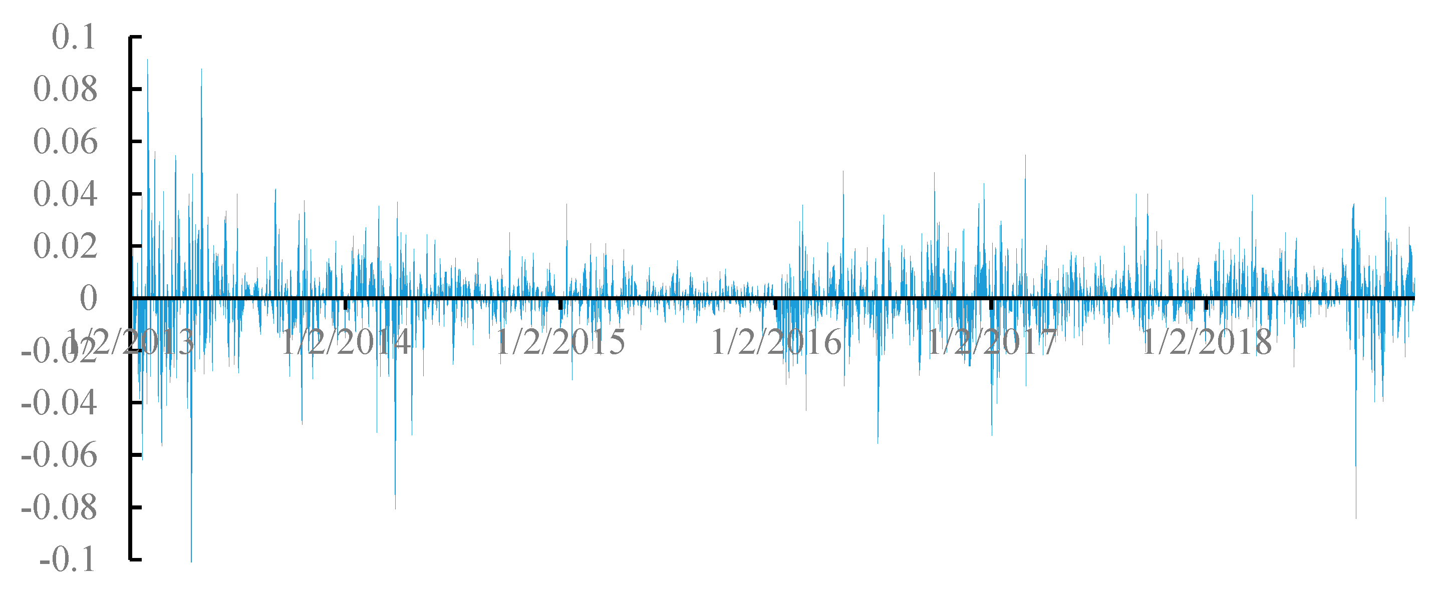
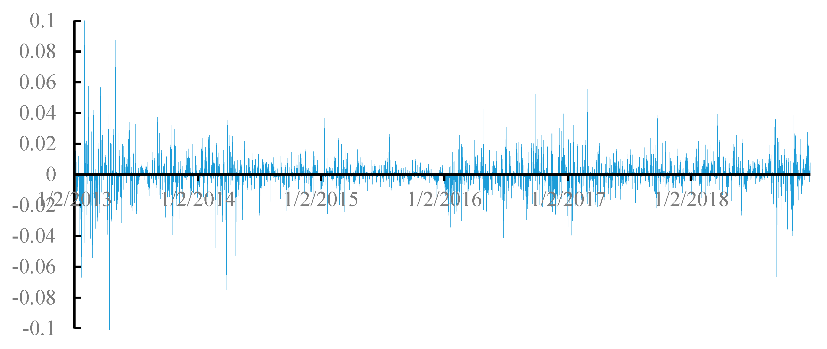
As described in Figure 1, the prices of EEX EUA spot and futures are generally increasing during the whole sample period, despite a decreasing period in the first half of 2016. The increasing may be mainly attributed to the emphasis on carbon reduction of the EU. Intuitively, the EUA spot price is less than €10 per ton in almost all of the sample period. Meanwhile, the EUA futures price is generally under €20 per ton before 2018. From Figure 1, it is obvious that the futures price is higher than the spot price as the yellow line representing the futures price is above the blue line representing the spot price, which may be mainly due to the more active transactions of the futures market than that of the spot market. Moreover, we can also find that the two prices change almost synchronously. For an in-depth comparative analysis of the two prices, we further calculate the correlation coefficient and the log returns of the prices by r t = log ( p t / p t 1 ) , and display the results in the following Table 1, Figure 2 and Figure 3, respectively.
The results in Table 1 show that the magnitude of the two correlation coefficients, i.e., the correlation of the two price series, and the correlation of the two return series, is close to one, which indicates that the price series and the return series of carbon spot and futures have a very close connection. Then, we can observe the two return series have almost the same tendency based on Figure 2 and Figure 3. For example, the two series were maximized at almost the same time during 2013. Furthermore, the returns fluctuate around zero. The return series changed seriously at the beginning of 2013, which may have been caused by the inconclusive policy orientation as the global carbon reduction environment changed in phase III. Moreover, some basic descriptive statistics of the two return series are shown in the following Table 2.
As summarized in the above Table 2, the maximum value of the EEX carbon spot and futures returns are 0.0915 and 0.1019, respectively. Meanwhile, the minimum values of the two returns are −0.1939 and −0.1834. The average returns of the two series are all approximately 0.0004. The magnitude of standard deviations is close to zero and the mean values are even smaller. Therefore, it is high for the volatilities of the two return series of carbon spot and futures. The kurtosis of carbon spot and futures returns exceeds three, and the skewness of these returns is not equal to zero. Such characteristics indicate that carbon spot and futures returns series have the characteristics of most financial time series [2,5]—namely, the series are not normally distributed and have heavy tails [5].
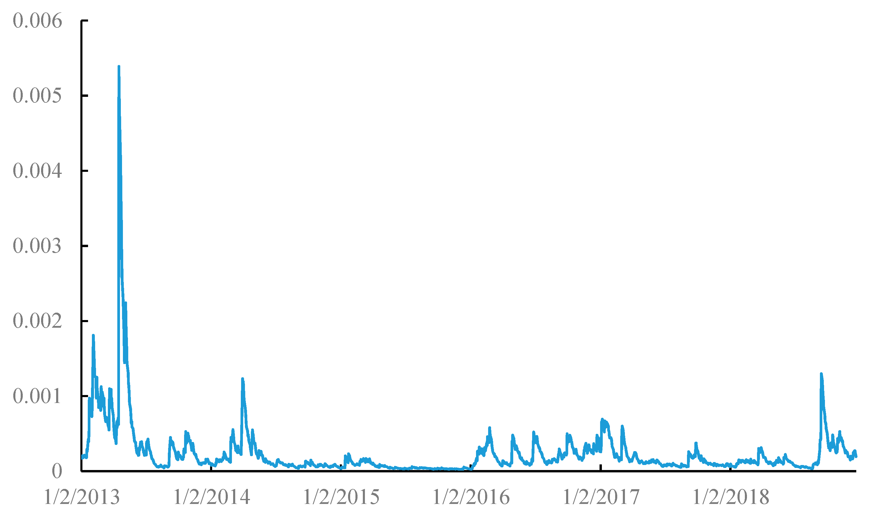
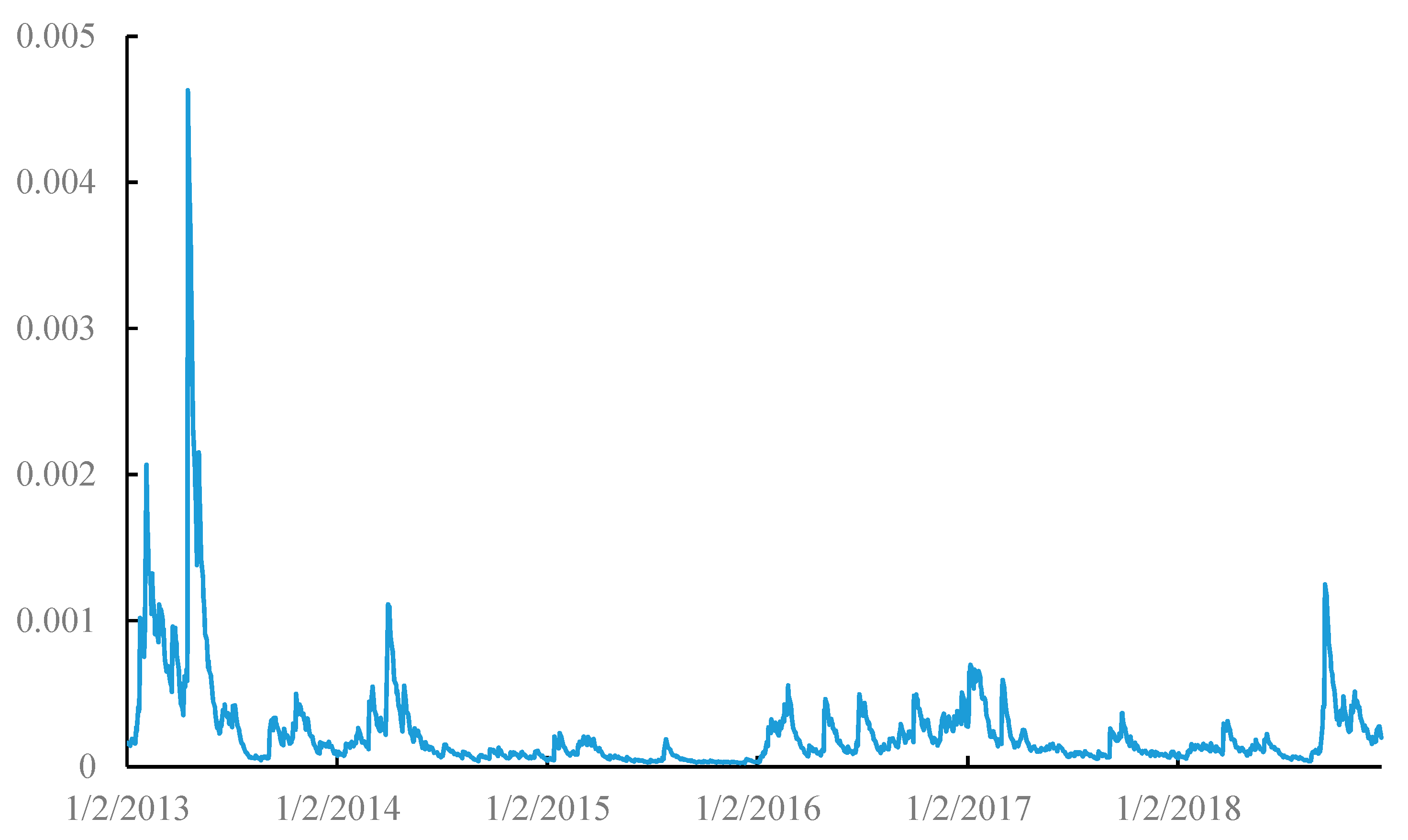
In most of the cases, the univariate GARCH model is apparently successful in estimating and forecasting the volatility of the financial time series data by existing literature [34,35,36,37,38]. Besides, according to previous researches [35,38,39], GARCH (1, 1) is selected as the appropriate model for the volatility estimating. We assume a generalized error distribution and calculate the conditional variances of carbon spot and futures and show the results in Figure 4 and Figure 5.
Intuitively, carbon spot and futures returns were volatile in the first half of 2013, the conditional variances reached the maximum in the sample period, and the entrance of Phase III may explain the phenomenon as significant changes occurred in the cap-and-trade system and the prohibition of banking of residual allowances [40]. Besides, the results in Figure 4 and Figure 5 consist with the finding of Kim [40] and Zhang [2], whose research sample period covers Phase III. In addition, it can also be noticed that compared with the variances in each calendar year, the variation at the beginning of each year is much more volatile, which may be ascribed to the “yearly complaint event.” From the above two figures, we may also find that the two conditional volatility series have almost the same tendency especially when it comes to extreme value.

4.2. DCC-GARCH Model

We select the DCC-GARCH model to identify the dynamic correlation between carbon spot and futures. The model has been developed by Engle [41], which is a natural extension of the constant correlation coefficient (CCC)-GARCH [42] model. There are two advantages of the DCC-GARCH model. On the one hand, the model detects possible changes in conditional correlations over time [43,44]; on the other hand, the model accounts the heteroscedasticity as the correlation coefficients of standardized residuals are estimated [45]. The variances are adjusted depending on the variance equation, and thus, the DCC estimator is unbiased. Hence, the DCC-GARCH model has become an excellent measure for correlation [46]. There are two steps of the DCC estimation process; the first step is to estimate a univariate GARCH model, and the second step refers to the estimation of time-varying conditional correlations. The model is defined in the following Equations (1)–(5).
X t = μ t + H t 1 / 2 ε t
H t = D t R t D t
R t = Q t 1 Q t Q t 1
D t = diag ( h 11 , t , , h NN , t )
Q t = ( 1 α β ) Q ¯ + α Q t 1 + β δ i , t 1 δ j , t 1
where Xt and μt represents the past observations and the conditional returns, respectively. Ht is the time-varying conditional variances, εt is the vector for the standardized residuals, Rt is a symmetric conditional correlation matrix, Dt is a diagonal matrix containing standard deviations of the returns estimated by the univariate GARCH model, and hii,t (i = 1, …, N) represents the diagonal elements of Ht. In the above equation, δ i , t is calculated as δ i , t = ε i , t / h i , t , where εi,t is the ith element in εt and hi,t is the ith element of the vector (hii,1,…,hii,t). Q ¯ represents the unconditional correlation matrixes. Besides, the model requires both α and β in Equation (5) are non-negative, and α + β < 1. Q t * is a diagonal matrix with the square root of the ith diagonal element of Qt on its corresponding location. For more details, you may refer to Celık [47].

4.3. VAR-BEKK-GARCH Model

According to existing research, the DCC-GARCH model can only capture the inter-relationship between different financial markets. However, the direction of the relationship estimated by the model, i.e., volatility spillovers from one market to other markets, cannot be inferred from the DCC-GARCH model [47]. For an in-depth understanding of the relationship between the carbon spot and futures market, we adopt a widely used bivariate BEKK-GARCH model [48,49,50,51,52] to test the direction of the relationship. The BEKK-GARCH model allows the conditional variances and co-variances to be interacted. Besides, the BEKK-GARCH model does not need to estimate so much parameters. Furthermore, the co-variance matrix is positive defined in the calculation process. Moreover, the VAR model is a linear predictability model, which allows the return on assets to be predicted by past values of predictors. According to previous studies [53,54,55], the VAR model is widely used in estimating and predicting asset returns as it can effectively reduce the transaction cost. For the perfect fitness of the VAR model on asset return, we update the mean equation of the BEKK-GARCH model by employing the VAR model. In this paper, we select the VAR-BEKK-GARCH model to analyze the volatility spillovers between carbon spot and futures markets. Specifically, the VAR-BEKK model can be summarized as follows in Equations (6)–(8).
R t = c + i = 1 p R t i + ε t
ε t ~ N ( 0 , H t )
H t = CC + B H t 1 B + A ε t 1 ε t 1 A
where Rt represents the return matrix, c is the conditional return, and εt refers to the residual. As for Ht, it is the conditional-variance-covariance matrix. And the matrix B is the parameter matrix with conditional variances, representing the relationships of the variances between different assets. The matrix A captures the ARCH effect, and the matrix D reflects the GARCH effect. For more details, you may refer to Yu [56].

5. Empirical Results

5.1. Dynamic Correlation of the EEX EUA Carbon Spot and Futures

A prerequisite of GARCH modeling is that the series need to be stable. Thus, before establishing the GARCH models for analyzing the correlation between EUA carbon spot and futures, it is essential to test the stationarity of the two return series. We exhibit the stationarity results by the augmented Dickey–Fuller (ADF) test in the following Table 3.
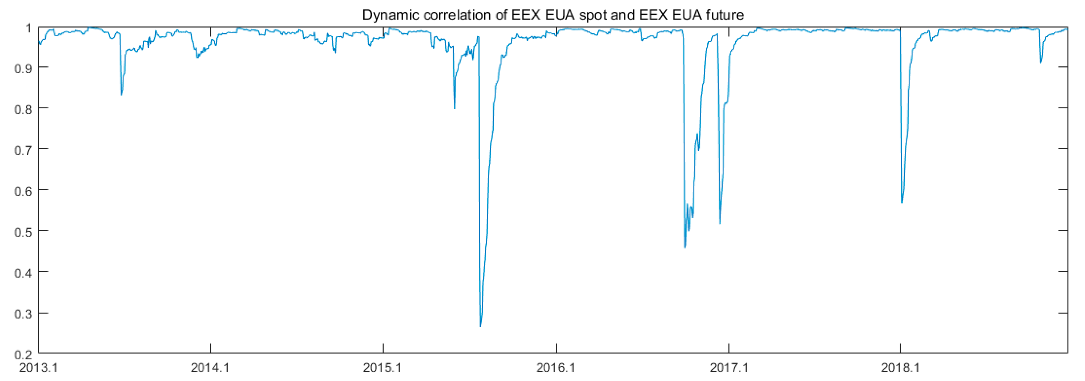
As seen in Table 3, the results for the return series of carbon spot and futures prices reject the null hypothesis of the ADF test as the values of the t-statistic are equal to 0.0000, which means that the two series are both stationary. Thus, this approach can be further used for GARCH modeling. According to existing researches [57,58,59], DCC-GARCH (1, 1) can efficiently capture the dynamic correlation between assets. Thus, in this paper, we chose the model to summarize the dynamic correlation between carbon spot and futures and the related result is shown in Figure 6.
We conduct a T-test to further identify whether the mean value of the correlation series is equal to a constant, i.e., 0. The results in Table 4 indicate that the two markets are indeed correlated because the null hypothesis is rejected as the p-value of the t-test is equal to zero.
As presented in Figure 6, the EUA carbon spot and EUA futures are highly correlated. The correlation coefficients are over 0.9 for almost all of the sample period. Evidently, extreme values appeared in the second half of 2015 and 2016 and the beginning of 2018. The abnormalities may be attributed to the following reasons. First, the leaders of the G7 countries showed support on carbon reduction with a clear attitude for the first time in June 2015; they pledged to realize a 40–70% carbon reduction in 2050 compared with 2010. The announcement may account for the volatility of futures prices compared with the ordinary moments, as seen in Figure 3 in the time period of June 2015. Meanwhile, the spot price did not change considerably, as shown in Figure 2, which may be the reason for the reduced correlation at that time. Second, in December 2016, the European Parliament Committee on Environment, Public Health and Food Safety reached an agreement on a reform scheme for the EU-ETS after 2020. As shown in Figure 2 and Figure 3, the agreement caused severe changes in carbon spot and futures prices, given that the EU approved that the emitters could save allowances for the next stage, which may account for the abnormal value in the second half of 2016. Third, at the end of 2017, the EU reached an agreement on the regulatory framework of the EU-ETS in Phase IV, and it may be one of the reasons for the drastic decrease in the correlation.

5.2. Volatility Spillover between the EEX EUA Carbon Spot and Futures

In this section, we first show the lag length selection criteria of the VAR model in the following Table 5.
According to the information criterion, the lag length selected in the VAR model is 8. As for the variance equation, we choose the widely used (1, 1) as the lag length for the ARCH and GARCH term [48,49,50,51,52]. The estimation results of the VAR (8)-BEKK (1, 1)-GARCH model is exhibited in the following Table 6.
In Table 6, A (i, j), B (i, j) and C (i, j) are the elements of the matrix A, B, and C described in Equation (9) in Secton 4.3. As for the volatility spillover, the parameters of A (i, j) and B (i, j) are of interest, as the parameters reflect the ARCH effect and GARCH effect, respectively. According to the parameters, we can obtain the following conclusions. First, the current conditional variance is positively affected by its previous ARCH term as the parameters of A (1, 1) and A (2, 2) are statistically significant at the 1% level. Second, the current conditional variance is closely related to the GARCH term, i.e., the conditional variance in the last period, as B (1, 1) and B (2, 2) are still significant. Third, the parameters of A (1, 1), A (2, 2), B (1, 1), and B (2, 2) are all significant, which means that carbon spot and futures all show volatility clustering.
Investigating the off-diagonal elements of matrix A and B, which capture cross-market effects, namely shock and volatility spillovers, respectively, we have several interesting discoveries. First, the ARCH term has a negative impact on other’s conditional variances since A (1, 2) and A (2, 1) are statistically negative, while the GARCH term has a positive effect as B (1, 2) and B (2, 1) are statistically significant. Second, there exists a bi-directional volatility spillover between carbon spot and futures as the parameters of A (1, 2), B (1, 2), A (2, 1) and B (2, 1) are all significant at the level of 1%. It means that the information embedded in price innovations of carbon spot as well as carbon futures indeed transmit to volatility. The reason of the volatility spillover is that the micro-foundation, market investors, and information source are almost the same for carbon spot and futures. These common factors will lead to volatility linkages by altering expectations, and thereby affecting asset demand, or cross-market hedging [60,61]. Moreover, carbon futures exhibits a higher degree of volatility spillover to carbon spot than reverse spillover mechanism since the values of A (1, 2) and B (1, 2) over that of A (2, 1) and B (2, 1). It infers that carbon futures have the function of price discovery to some extent. The existence of volatility spillover helps to construct the optimal hedging ratio, which benefits the carbon investors in the futures. We elaborate this point in the next section.
To further verify the validity of the volatility spillover exhibited in Table 6, we conduct the Wald test shown in Table 7. The results of the Wald test support the above conclusions that the volatility of carbon futures can impact on that of carbon spot, vice versa.

5.3. Hedge Ratios and Hedging Effectiveness

In this section, we examine the implications of the aforementioned results of the VAR-BEKK-GARCH model for hedging strategy and portfolio management. Based on the modern portfolio theory, Johnson [62] proposed the well-known minimum variance hedge ratio model for minimizing the risk associated with a certain portfolio. Assume asset j can be used as a hedge for another asset i. The return of a hedged portfolio can be written as follows in Equation (9).
R H , t = R s , t γ f , t R f , t
where RH,t represents the return of the hedged portfolio, γf,t is the hedge ratio, Rs,t and Rf,t represent the return of spot and futures return respectively. According to Johnson [62], Baillie [63], and Kroner [64], the optimal holding weight of the carbon spot and futures can be determined by the following equations in (10), (11) and (12).
w sf , t = h t ss h t sf h t ff 2 h t sf + h t ss
w sf , t = { 0 , if   w sf , t < 0 w sf , t , if   0 < w sf , t < 1 1 , if   w sf , t > 1
γ f , t * = h t sf h t ff
In the above expressions, wsf,t represents the weight of carbon futures in one unit portfolio including carbon spot and futures. h t sf represents the co-variance between carbon spot and futures, which is estimated by the multivariate GARCH model. h t ss and h t ff denote the variance of carbon spot and futures, respectively. γ f , t * is the optimal hedge ratio.
In order to evaluate the effectiveness of the constructed hedging strategy, we further calculate a hedging effectiveness (HE) value, which is adopted by Ku [65]. The calculation of HE value is shown as follows.
HE = var unhedged var hedged var unhedged
where the variances of the hedge portfolio, namely varhedged, are obtained from the variance of the rate of return, RH,t. The variance of the unhedged portfolio is the variance of spot returns (see, for example, Ripple and Moosa [66]. The closer the HE tends to one, the higher hedging effectiveness and better risk reduction. Some basic results of the above-mentioned equations are shown in Table 8.
As can be seen from Table 8, the optimal hedge ratio for carbon futures is 0.9468. This means that a unit of long position in carbon spot can be hedged by shorting 0.9468 of carbon futures in average. Moreover, the weight for carbon futures in the portfolio including carbon spot and futures is 0.4208, while the weight for carbon spot is 0.5292. Furthermore, the HE value is 0.9370, which indicates that around 94% of price return variance of the carbon spot can be effectiveness hedged by taking a short position in carbon futures into the portfolio

6. Further Discussion

In this section, we provide further discussion on the correlation between carbon spot and carbon futures markets by replacing our dataset with the trading data in phase II of the EU-ETS. Due to the data availability, the data scope for the prices of carbon spot and futures are from 27 October 2009 to 31 December 2012. Some basic characteristics of the new data in phase II is shown in Table 9.
Then, we employ the same methods as in Section 5 to further discuss the correlation between carbon spot and futures, and the detailed results are shown as follows.
The ADF test results of the two return series and the estimation results of the DCC-GARCH model are exhibited in the following Table 10 and Figure 7. Specifically, the results of the ADF test show that the returns of carbon spot and futures are still stationary and thus can be used for subsequent GARCH modeling. The results of dynamic correlation indicate that there exists an obvious dynamic linkage between carbon spot and futures. Similar to our research for phase III of the EU-ETS, we still conduct a T-test to further certify whether the two markets are correlated, and the results shows the correlation between carbon spot and futures to be dynamic.
We further show the lag length selection process of the VAR model in Table 11.
As shown in Table 11, the lag length selected for the VAR model in phase II of the EU ETS is 4. The estimation results for VAR (4)-BEKK (1, 1)-GARCH model is shown in Table 12. The results exhibit that there exists a volatility spillover from carbon futures to carbon spot in phase II of the EU ETS as the parameters of A (1, 2) and B (1, 2) are significant at the level of 1%. The reverse volatility spillover from carbon spot to carbon futures is relatively weaker as the parameters of B (2, 1) is not significant. Moreover, the results of the Wald test shown in Table 13 further support this conclusion for the rejection of the null hypothesis of volatility spillover from carbon spot to carbon futures. Thus, the volatility spillover effect in phase II of the EU ETS is relative weaker than that in phase III. This further demonstrates the importance of researching the phase III of the EU ETS as the more volatility spillover between carbon spot and futures.
Similar with the analysis in the above section, we further provide the hedge ratio and HE value to evaluate the effectiveness of the hedge strategy in phase II of the EU ETS. And the results are shown in the following Table 14. Here, we can conclude that the hedging effectiveness of phase II is lower than that of phase III for the HE value is obviously under 0.9370—namely, the HE value in phase III.
In general, the correlation between carbon spot and futures becomes closer in phase III of the EU ETS when compared with the phase II, as the mean value of dynamic correlation shown in Figure 6 is relatively higher than the correlation in Figure 7. Moreover, the volatility effect is more intense in phase III of the EU ETS than that in phase III for the parameters of A (2, 1) is significant at a level of 10% and that of B (2, 1) is not significant. As to the hedging strategy based on the VAR-BEKK-GARCH model, it is obvious that the hedging strategy performs better in phase III than phase II as the HE value is relatively higher in phase III. Thus, we can deduce the conclusions that the carbon futures market in phase III of the EU ETS is a more applicable market to hedge risk from carbon spot market when compared with the market in phase II.

7. Conclusions

In this paper, we collect our data set of carbon spot and futures market in phase III of the EU-ETS to analyze the dynamic correlation and volatility spillover of the two markets. The novelty of this paper is that it extends the time scale of existing research to phase III of the EU-ETS and makes a comprehensive analysis for the carbon spot-futures linkages. Our empirical results of the DCC-GARCH model show that carbon spot and carbon futures are highly correlated. Meanwhile, the empirical results of the VAR-BEKK-GARCH model indicate that there exist significantly bi-directional volatility spillovers between the two carbon markets. Besides, we construct a hedge strategy based on the results of VAR-BEKK-GARCH model, and the results denote that the carbon futures market is a good market for investors who want to hedge risk from carbon spot market. Moreover, we make a further exploration on the correlation of carbon spot and futures by replacing our data set with the trading data in phase II of the EU-ETS. The results do not change our conclusions on dynamic correlation and volatility spillover. But another interesting issue is found that carbon futures market in phase III of the EU ETS can better hedge the risk from carbon spot market when compared with phase II. Our empirical results further help to better understand the carbon spot-futures linkages in the EU-ETS. Besides, our results benefit those investors who invest in both carbon spot and futures market to effectively hedge risk.
There are indeed alternative methods to estimate dynamic correlation relationship between carbon spot and futures or even more assets. Such as, Orthogonal GARCH (O-GARCH) model [2,5], Copula-DCC-GARCH model [67], ADCC-EGARCH model [68], et al. In this paper, we only select the DCC-GARCH model as the basic estimating method to explore the relationship between carbon spot and futures. And these alternative methods will be carefully employed in our futures research. Moreover, in Section 5.3, we construct a portfolio composed of carbon assets without any other assets. Thus, we try to include more assets, i.e., energy assets, financial assets and commodity assets, into the portfolios in the futures research, which may be benefit the investors globally.

Author Contributions

H.C. collected the data and wrote the original manuscript; Z.L. provided the methodologies used in this paper; Y.Z. implemented the empirical process in this paper; Y.W. provided the idea and polished the paper. All authors have read and agreed to the published version of the manuscript.

Funding

This research was supported by the scientific research start-up fund for young teachers in Beijing Technology and Business University under No. QNJJ2020-36 and the Sugar Crop Research System, CARS (CARS-170601). And it was also supported by the Research Base of Capital Circulation Industry under No. JD-ZD-2020-001.

Acknowledgments

We would like to express our great thanks to the editor and anonymous reviewers, any remaining errors belong to the authors.

Conflicts of Interest

The authors declare no conflict of interest.

References

  1. Hughes, T.P.; Baird, A.H.; Bellwood, D.R.; Card, M.; Connolly, S.R.; Folke, C.; Grosberg, R.; Hoegh-Guldberg, O.; Jackson, J.B.C.; Kleypas, J.; et al. Climate change, human impacts, and the resilience of coral reefs. Science 2003, 301, 929–933. [Google Scholar] [CrossRef] [Green Version]
  2. Zhang, Y.; Liu, Z.; Yu, X. The Diversification Benefits of Including Carbon Assets in Financial Portfolios. Sustainability 2017, 9, 437. [Google Scholar] [CrossRef] [Green Version]
  3. Trück, S.; Härdle, W.; Weron, R. The Relationship between Spot and Futures CO2 Emission Allowance Prices in the EU-ETS. SSRN Electron. J. 2012, 144, 1147–1155. [Google Scholar] [CrossRef] [Green Version]
  4. EU Emissions Trading System|Climate Change. Available online: https://ec.europa.eu/clima/policies/ets_en (accessed on 23 March 2020).
  5. Luo, C.; Wu, D. Environment and economic risk: An analysis of carbon emission market and portfolio management. Environ. Res. 2016, 149, 297–301. [Google Scholar] [CrossRef] [PubMed] [Green Version]
  6. Arouri, M.E.H.; Jawadi, F.; Nguyen, D.K. Nonlinearities in carbon spot-futures price relationships during Phase II of the EU ETS. Econ. Model. 2012, 29, 884–892. [Google Scholar] [CrossRef]
  7. Kang, S.H.; Lee, J.W. The network connectedness of volatility spillovers across global futures markets. Phys. A 2019, 526, 120756. [Google Scholar] [CrossRef]
  8. Rittler, D. Price discovery and volatility spillovers in the European Union emissions trading scheme: A high-frequency analysis. J. Bank. Financ. 2012, 36, 774–785. [Google Scholar] [CrossRef]
  9. Website in Chinese. Available online: http://www.tanpaifang.com/tanjiaoyi/2012/1215/10637.html (accessed on 23 March 2020).
  10. Kamdem, J.S.; Nsouadi, A.; Terraza, M. Time-frequency analysis of the relationship between EUA and CER carbon markets. Environ. Model. Assess. 2016, 21, 279–289. [Google Scholar] [CrossRef]
  11. Website in Chinese. Available online: www.tanjiaoyi.com/article-24219-1.html (accessed on 23 March 2020).
  12. Baba, Y.; Engle, R.F.; Kraft, D.F.; Kroner, K.F. Multivariate Simultaneous Generalized ARCH; Department of Economics, University of California: San Diego, CA, USA, 1990. [Google Scholar]
  13. Taschini, L.; Paolella, M.S. An econometric analysis of emission trading allowances. J. Bank. Financ. 2008, 32, 06–26. [Google Scholar] [CrossRef] [Green Version]
  14. Benz, E.; Trück, S. Modeling the price dynamics of CO2 emission allowances. Energy Econ. 2009, 31, 4–15. [Google Scholar] [CrossRef]
  15. Benz, E.A.; Hengelbrock, J. Price discovery and liquidity in the European CO2 futures market: An intraday analysis. In Proceedings of the 2018 Finance International Meeting AFFI-EUROFIDAI, Paris, France, 20 December 2018. [Google Scholar]
  16. Daskalakis, G.; Markellos, R.N. Are the European carbon markets efficient? Rev. Futures Mark. 2008, 17, 103–128. [Google Scholar]
  17. Feng, Z.H.; Zou, L.L.; Wei, Y.M. Carbon price volatility: Evidence from EU ETS. Appl. Energy 2011, 88, 590–598. [Google Scholar] [CrossRef]
  18. Zhang, Y.; Liu, Z.; Xu, Y. Carbon price volatility: The case of China. PLoS ONE 2018, 13, e0205317. [Google Scholar] [CrossRef] [PubMed] [Green Version]
  19. Silvapulle, P.; Moosa, I.A. The relationship between spot and futures prices: Evidence from the crude oil market. J. Futures Mark. 1999, 19, 175–193. [Google Scholar] [CrossRef]
  20. Li, P.; Zhang, Z.; Yang, T.; Qingchao, Z. The relationship among China’s fuel oil spot, futures and stock markets. Financ. Res. Lett. 2018, 24, 151–162. [Google Scholar] [CrossRef]
  21. Shao, Y.; Yang, Y.; Shao, H.; Stanley, H.E. Time-varying lead–lag structure between the crude oil spot and futures markets. Phys. A 2019, 523, 723–733. [Google Scholar] [CrossRef]
  22. George, M.; Roselyne, J. Pricing efficiency and arbitrage in the EU ETS carbon futures market. J. Invest. Strategy 2007, 2, 23–26. [Google Scholar]
  23. Uhrig-Homburg, M.; Wagner, M. Futures price dynamics of CO2 emission allowances: An empirical analysis of the trial period. J. Deriv. 2009, 17, 73–88. [Google Scholar] [CrossRef] [Green Version]
  24. Joyeux, R.; Milunovich, G. Testing market efficiency in the EU carbon futures market. Appl. Financ. Econ. 2010, 20, 803–809. [Google Scholar] [CrossRef]
  25. Chevallier, J. A note on cointegrating and vector autoregressive relationships between CO2 allowances spot and futures prices. Econ. Bull. 2010, 30, 1564–1584. [Google Scholar]
  26. Niblock, S.J.; Harrison, J.L. Do dynamic linkages exist among European carbon markets? Int. Bus. Econ. Res. J. 2012, 11, 33–44. [Google Scholar] [CrossRef] [Green Version]
  27. Gorenflo, M. Futures price dynamics of CO2 emission allowances. Empir. Econ. 2013, 45, 1025–1047. [Google Scholar] [CrossRef]
  28. Balcılar, M.; Demirer, R.; Hammoudeh, S.; Nguyen, D.K. Risk spillovers across the energy and carbon markets and hedging strategies for carbon risk. Energy Econ. 2016, 54, 159–172. [Google Scholar] [CrossRef] [Green Version]
  29. European Union Emission Trading System (EU ETS). Available online: https://www.emissions-euets.com/carbon-market-glossary/872-european-union-emissions-trading-system-eu-ets (accessed on 23 March 2020).
  30. Stavins, R.N. Experience with market-based environmental policy instruments. In Handbook of Environmental Economics; Mäler, K., Vincent, J.R., Eds.; Elsevier: Amsterdam, The Netherlands, 2003; Volume 1, pp. 355–435. [Google Scholar]
  31. Website in Chinese. Available online: http://www.tanpaifang.com/tanjiaoyi/2015/0122/41884.html (accessed on 23 March 2020).
  32. Verbruggen, A.; Laes, E.; Woerdman, E. Anatomy of emissions trading systems: What is the EU ETS? Environ. Sci. Policy 2019, 98, 11–19. [Google Scholar] [CrossRef]
  33. Monitoring, Reporting and Verification of EU ETS Emissions|Climate Change. Available online: https://ec.europa.eu/clima/policies/ets/monitoring_en (accessed on 23 March 2020).
  34. Abdalla, S.Z.S.; Winker, P. Modelling stock market volatility using univariate GARCH models: Evidence from Sudan and Egypt. Int. J. Financ. Econ. 2012, 4, 161–176. [Google Scholar] [CrossRef]
  35. Efimova, O.; Serletis, A. Energy markets volatility modelling using GARCH. Energy Econ. 2014, 43, 264–273. [Google Scholar] [CrossRef]
  36. Karmakar, M. Modeling conditional volatility of the Indian stock markets. Vikalpa J. Decis. Mak. 2005, 30, 21–37. [Google Scholar] [CrossRef] [Green Version]
  37. Lin, S.X.; Tamvakis, M.N. Spillover effects in energy futures markets. Energy Econ. 2001, 23, 43–56. [Google Scholar] [CrossRef]
  38. Morana, C. A semiparametric approach to short-term oil price forecasting. Energy Econ. 2001, 23, 325–338. [Google Scholar] [CrossRef]
  39. Oberholzer, N.; Venter, P. Univariate GARCH models applied to the JSE/FTSE stock indices. Procedia Econ. Financ. 2015, 24, 491–500. [Google Scholar] [CrossRef] [Green Version]
  40. Kim, J.; Park, Y.J.; Ryu, D. Stochastic volatility of the futures prices of emission allowances: A Bayesian approach. Phys. A 2017, 465, 714–724. [Google Scholar] [CrossRef]
  41. Engle, R. Dynamic conditional correlation: A simple class of multivariate generalized autoregressive conditional heteroskedasticity models. J. Bus. Econ. Stat. 2002, 20, 339–350. [Google Scholar] [CrossRef]
  42. Bollerslev, T. Modelling the coherence in short-run nominal exchange rates: A multivariate generalized ARCH model. Rev. Econ. Stat. 1990, 72, 498–505. [Google Scholar] [CrossRef]
  43. Corsetti, G.; Pericoli, M.; Sbracia, M. ‘Some contagion, some interdependence’: More pitfalls in tests of financial contagion. J. Int. Money Financ. 2005, 24, 1177–1199. [Google Scholar] [CrossRef]
  44. Syllignakis, M.N.; Kouretas, G.P. Dynamic correlation analysis of financial contagion: Evidence from the Central and Eastern European markets. Int. Rev. Econ. Financ. 2011, 20, 717–732. [Google Scholar] [CrossRef]
  45. Chiang, T.C.; Jeon, B.N.; Li, H. Dynamic correlation analysis of financial contagion: Evidence from Asian markets. J. Int. Money Financ. 2007, 26, 1206–1228. [Google Scholar] [CrossRef]
  46. Cho, J.H.; Parhizgari, A.M. East Asian financial contagion under DCC-GARCH. Int. J. Bank. Financ. 2008, 6, 17–30. [Google Scholar]
  47. Celık, S. The more contagion effect on emerging markets: The evidence of DCC-GARCH model. Econ. Model 2012, 29, 1946–1959. [Google Scholar] [CrossRef]
  48. Rahman, S.; Serletis, A. Oil price uncertainty and the Canadian economy: Evidence from a VARMA, GARCH-in-Mean, asymmetric BEKK model. Energy Econ. 2012, 34, 603–610. [Google Scholar] [CrossRef]
  49. Yan, Z.; Li, S. Hedge ratio on Markov regime-switching diagonal Bekk–Garch model. Financ. Res. Lett. 2018, 24, 49–55. [Google Scholar] [CrossRef]
  50. Oliveira, F.A.; Maia, S.F.; Jesus, D.P.; da Cássio, B.N. Which information matters to market risk spreading in Brazil? Volatility transmission modelling using MGARCH-BEKK, DCC, t-Copulas. N. Am. J. Econ. Financ. 2018, 45, 83–100. [Google Scholar] [CrossRef]
  51. Lin, A.J.; Chang, H.Y.; Hsiao, J.L. Does the Baltic Dry Index drive volatility spillovers in the commodities, currency, or stock markets? Transp. Res. E Logist. Transp. Rev. 2019, 127, 265–283. [Google Scholar] [CrossRef]
  52. Katsiampa, P.; Corbet, S.; Lucey, B. Volatility spillover effects in leading cryptocurrencies: A BEKK-MGARCH analysis. Financ. Res. Lett. 2019, 29, 68–74. [Google Scholar] [CrossRef] [Green Version]
  53. Guidolin, M.; Hyde, S. Can VAR models capture regime shifts in asset returns? A long-horizon strategic asset allocation perspective. J. Bank. Financ. 2012, 36, 695–716. [Google Scholar] [CrossRef] [Green Version]
  54. Anggraeni, W.; Andri, K.B.; Mahananto, F. The performance of ARIMAX model and Vector Autoregressive (VAR) model in forecasting strategic commodity price in Indonesia. Procedia Comput. Sci. 2017, 124, 189–196. [Google Scholar] [CrossRef]
  55. Zhang, Y.; Lin, J. Can the VAR model outperform MRS model for asset allocation in commodity market under different risk preferences of investors? Int. Rev. Financ. Anal. 2019, 66. [Google Scholar] [CrossRef]
  56. Yu, L.; Zha, R.; Stafylas, D.; He, K.; Liu, J. Dependences and volatility spillovers between the oil and stock markets: New evidence from the copula and VAR-BEKK-GARCH models. Int. Rev. Financ. Anal. 2019. [Google Scholar] [CrossRef]
  57. Akkoc, U.; Civcir, I. Dynamic linkages between strategic commodities and stock market in Turkey: Evidence from SVAR-DCC-GARCH model. Resour. Policy 2019, 62, 231–239. [Google Scholar] [CrossRef]
  58. Hou, Y.; Li, S.; Wen, F. Time-varying volatility spillover between Chinese fuel oil and stock index futures markets based on a DCC-GARCH model with a semi-nonparametric approach. Energy Econ. 2019, 83, 119–143. [Google Scholar] [CrossRef]
  59. Shiferaw, Y.A. Time-varying correlation between agricultural commodity and energy price dynamics with Bayesian multivariate DCC-GARCH models. Phys. A 2019, 526, 120807. [Google Scholar] [CrossRef]
  60. Miao, H.; Ramchander, S.; Wang, T.; Yang, D. Role of index futures on China’s stock markets: Evidence from price discovery and volatility spillover. Pac. Basin Financ. J. 2017, 44, 13–26. [Google Scholar] [CrossRef]
  61. Fassas, A.P.; Siriopoulos, C. Intraday price discovery and volatility spillovers in an emerging market. Int. Rev. Econ. Financ. 2019, 59, 333–346. [Google Scholar] [CrossRef]
  62. Johnson, L.L. The theory of hedging and speculation in commodity futures. In The Economics of Futures Trading; Palgrave Macmillan: London, UK, 1976; pp. 83–99. [Google Scholar]
  63. Baillie, R.T.; Myers, R.J. Bivariate GARCH estimation of the optimal commodity futures hedge. J. Appl. Econ. 1991, 6, 109–124. [Google Scholar] [CrossRef]
  64. Kroner, K.F.; Ng, V.K. Modeling asymmetric movement of asset prices. Rev. Financ. Stud. 1998, 11, 844–871. [Google Scholar] [CrossRef]
  65. Ku, Y.H.; Chen, H.; Chen, K. On the application of the dynamic conditional correlation model in estimating optimal time-varying hedge ratios. Appl. Econ. Lett. 2007, 14, 503–509. [Google Scholar] [CrossRef]
  66. Ripple, R.D.; Moosa, I.A. Hedging effectiveness and futures contract maturity: The case of nymex crude oil futures. Appl. Econ. Lett. 2007, 17, 683–689. [Google Scholar] [CrossRef]
  67. Kim, J.; Jung, H. Linear time-varying regression with Copula–DCC–GARCH models for volatility. Econ. Lett. 2016, 145, 262–265. [Google Scholar] [CrossRef]
  68. Kocaarslan, B.; Soytas, U. Dynamic correlations between oil prices and the stock prices of clean energy and technology firms: The role of reserve currency (US dollar). Energy Econ. 2019, 84. [Google Scholar] [CrossRef]
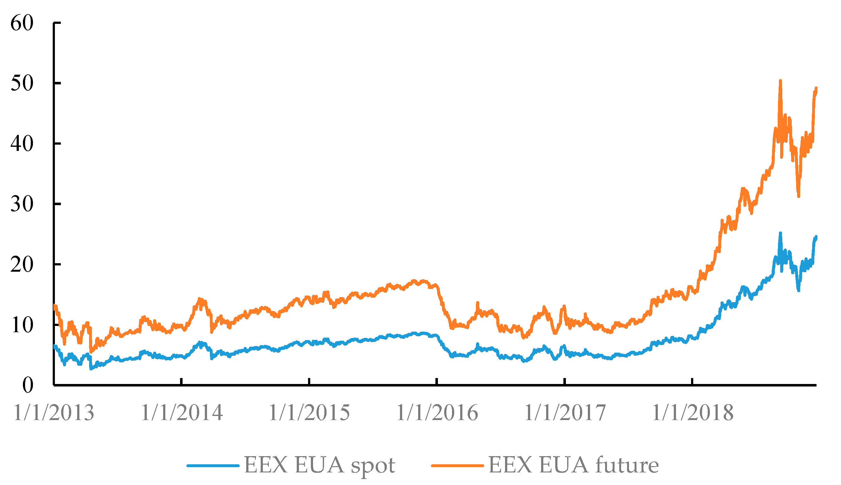
Figure 1. Price trend of EEX (European Energy Exchange) EUA (European Union allowance) spot and futures.
Sustainability 12 02517 g001
Figure 2. EEX EUA spot return in phase III of the European Union Emission Trading Scheme (EU-ETS).
Sustainability 12 02517 g002
Figure 3. EEX EUA futures return in phase III of the EU-ETS.
Sustainability 12 02517 g003
Figure 4. Conditional variance of EEX EUA carbon spot return.
Sustainability 12 02517 g004
Figure 5. Conditional variance of EEX EUA carbon futures return.
Sustainability 12 02517 g005
Figure 6. Dynamic correlation of EEX EUA spot and EEX EUA futures.
Sustainability 12 02517 g006
Figure 7. Dynamic correlation coefficient of carbon spot and futures in phase II of the EU-ETS.
Sustainability 12 02517 g007
Table 1. Correlation coefficient for carbon spot and carbon futures.
Correlation between Spot and Futures PriceFutures PriceCorrelation between Spot and Futures ReturnFutures Return
Spot price0.9999Spot return0.9680
Table 2. Descriptive statistics of the EEX EUA spot and futures returns.
EEX EUA ReturnMaxMinMeanStdSkewnessKurtosis
EEX EUA spot return0.0915−0.19390.00040.0148−1.446022.7711
EEX EUA futures return0.1019−0.18340.00040.0148−1.194319.5809
Table 3. ADF test of the returns of carbon spot and futures.
Carbon ReturnTypest-Statisticp-Value
Carbon spotIntercept−31.23850.0000
Trend and intercept−31.30780.0000
none−31.21540.0000
Carbon futuresIntercept −30.83120.0000
Trend and intercept−30.90400.0000
none−30.80950.0000
Note: Intercept, trend and intercept, and none mean three types of the augmented Dickey–Fuller (ADF) test with the intercept, trend and intercept and none, respectively. The null hypothesis of the ADF test assumes that the return series of carbon spot and futures have a unit root. The P-value represents the significance of the corresponding test.
Table 4. T-test for the dynamic correlation coefficient.
Null Hypothesist-Statisticp-ValueConclusion
The mean value of the correlation series is equal to 0436.96910.0000Refuse
Table 5. Lag length selection of the VAR model.
Lag OrderLogLLRFPEAICSCHQ
010,806.10-3.02×10⁻⁹−13.9408−13.9339−13.9382
110,987.22361.54272.41×10−9−14.1693−14.1486−14.1616
211,096.97218.78612.10×10−9−14.3058−14.2713−14.2929
311,140.8887.43631.99×10−9−14.3573−14.3090−14.3393
411,179.7177.19691.91×10−9−14.4022−14.3401−14.3791
511,251.37142.30571.75×10−9−14.4895−14.4136 *−14.4613 *
611,258.0413.22561.74×10−9−14.4930−14.4033−14.4596
711,267.2718.29101.73×10−9−14.4997−14.3962−14.4612
811,273.4412.2053 *1.72×10−9 *−14.5025 *−14.3852−14.4589
Note: LR, FPE, AIC, SC and HQ indicates the sequential modified LR test statistic, final prediction error, Akaike information criterion, Schwarz information criterion, and Hannan–Quinn information criterion, respectively. * denotes lag length selected by the criterion.
Table 6. Estimation results of the VAR-BEKK-GARCH model.
Matrix ElementCoefficientStd Errort-Statisticp-Value
C (1, 1)0.00090.00025.06410.0000
C (2, 1)0.00080.00023.71630.0002
C (2, 2)−0.00020.0001−3.67780.0002
A (1, 1)0.72430.013553.73920.0000
A (1, 2)−0.53330.0182−29.37060.0000
A (2, 1)−0.46050.0159−29.04770.0000
A (2, 2)0.79430.015551.17500.0000
B (1, 1)0.87130.0081107.94060.0000
B (1, 2)0.15450.004633.28100.0000
B (2, 1)0.09520.009110.41230.0000
B (2, 2)0.81360.0026307.26350.0000
Table 7. Results of the Wald test of volatility spillovers.
Volatility SpilloverNull HypothesisWald Testp-Value
From Carbon Spot to Carbon Futuresa21 = b21 = 01593.11520.0000
From Carbon Futures to Carbon Spota12 = b12 = 0843.91330.0000
Between Carbon Spot and Carbon Futuresa12 = b12 = a21 = b21 = 03478.88310.0000
Table 8. Optimal hedge ratio and hedging effectiveness in phase III of the EU-ETS.
Hedge CharacteristicOptimal Hedge Ratio Holding Weight Hedging Effectiveness
Value0.94680.42080.9370
Table 9. Basic characteristics of carbon spot and futures in phase II of the EU ETS.
Carbon ReturnMaxMinMeanStdSkewnessKurtosis
carbon spot return0.0812−0.0501−0.00040.01120.23945.1083
Carbon futures return0.0800−0.0498−0.00040.01110.02854.9962
Table 10. ADF test of carbon spot and futures returns in phase II of the EU ETS.
Carbon ReturnTypest-Statisticp-Value
Carbon spotIntercept−27.86400.0000
Trend and intercept−27.86100.0000
none−27.84510.0000
Carbon futuresIntercept −28.00240.0000
Trend and intercept−27.99590.0000
none−27.97880.0000
Note: Intercept, trend and intercept, and none mean that the three types of the ADF test with intercept, trend and intercept and none, respectively. The null hypothesis of the ADF test assumes that the return series of carbon spot and futures have a unit root. The P-value represents the significance of the corresponding test.
Table 11. Lag length selection of the vector autoregression (VAR) model in phase II.
Lag OrderLogLLRFPEAICSCHQ
05971.355-1.66×10⁻⁹−14.54167−14.53019−14.53727
16035.231127.28391.43×10−9−14.68753−14.65310−14.67432
26076.75282.537011.31×10−9−14.77893−14.72156−14.75692
36101.58749.245971.24×10−9−14.82969−14.74936 *−14.79887
46110.10316.84632 *1.23×10−9 *−14.84069 *−14.73741−14.80106 *
56110.9891.7474681.24×10−9−14.83310−14.70688−14.78467
66112.3102.6007401.25×10−9−14.82658−14.67740−14.76934
76115.4646.1928051.25×10−9−14.82452−14.65239−14.75847
86118.4575.8614811.25×10−9−14.82206−14.62699−14.74722
Note: LR, FPE, AIC, SC and HQ indicates the sequential modified LR test statistic, Final prediction error, Akaike information criterion, Schwarz information criterion and Hannan-Quinn information criterion, respectively. * denotes lag length selected by the criterion.
Table 12. Estimation results of the VAR-BEKK-GARCH model in phase II of the EU-ETS.
Matrix ElementCoefficientStd Errort-Statisticp-Value
C (1, 1)0.00070.00032.72630.0064
C (2, 1)0.00130.00043.11270.0019
C (2, 2)0.00100.00032.82210.0048
A (1, 1)0.43960.08265.31900.0000
A (1, 2)−0.28210.0854−3.30440.0010
A (2, 1)−0.16060.0836−1.91950.0549
A (2, 2)0.59110.08816.70630.0000
B (1, 1)0.88050.050917.29020.0000
B (1, 2)0.23420.05794.04710.0001
B (2, 1)0.08030.05201.54270.1229
B (2, 2)0.71320.059511.98860.0000
Table 13. Results of the Wald test of volatility spillovers in phase II of the EU-ETS.
Volatility SpilloverNull HypothesisWald Testp-Value
From Carbon Spot to Carbon Futuresa21 = b21 = 03.69260.1578
From Carbon Futures to Carbon Spota12 = b12 = 016.47550.0003
Between Carbon Spot and Carbon Futuresa12 = b12 = a21 = b21 = 087.13160.0000
Table 14. Optimal hedge ratio and hedging effectiveness in phase II of the EU-ETS.
Hedge CharacteristicOptimal Hedge Ratio Holding WeightHedging Effectiveness
Value0.90500.39170.8938