Spatio-Temporal Correlation Analysis of Air Quality in China: Evidence from Provincial Capitals Data

Abstract

In China, public health awareness is growing as people get more concerned about the air quality. Based on the air quality index (AQI) of 31 provincial capital cities (2015–2018) in China, we studied the spatio-temporal correlations of air quality between cities. With spatial, temporal and spatio-temporal analysis, we systematically obtained many interesting results where the traditional analyses may be lacking. Firstly, the air quality of cities has spatial spillover and agglomeration effects and further the spatial correlation becomes higher with time. Secondly, there exists temporal correlation between the current AQI and its past values on multiple time scales, which shows certain periodicity. Thirdly, due to the changing characteristics of time, social activities and other factors affect the air quality positively. However, with the panel data model, the coefficients of spatio-temporal correlation vary for different cities.

1. Introduction

Due to the rapid growth of industrialization and urbanization, the consumption of energy such as coal, natural gas and oil has increased rapidly in China. The air pollution is getting worse and worse [1]. The pollution problem has seriously affected people’s quality of life and the public’s health and has even caused certain obstacles to the sustainable development of the entire country. How to face and effectively deal with air pollution has become the focus of the whole society and its proper solution will significantly improve the living environment of the people and promote the harmonious development of social ecology [2].

The traditional perspective of research is to study the impact of specific pollutants on the urban air quality or to analyze the distribution characteristics of air quality only from the perspective of time or space [3]. However, spatial and temporal correlation analysis should be used in the study of air quality in Chinese cities. Spatial and temporal correlation analysis of air quality refers to the statistical analysis of the evolution characteristics of data sequences formed by the time evolution of points in all directions of space. In other words, it reflects the correlation of spatial and temporal data in time and space by studying the change law of spatial objects with time. From the perspective of the spatio-temporal correlation of air quality, this paper comprehensively analyzes the changing law of air quality among Chinese cities, which has certain significance for China to formulate relevant air pollution control policies.

This paper aims to reveal the spatial and temporal evolution of air quality of Chinese cities. It proceeds as follows: In Section 2, we review the literature and discuss the spatio-temporal correlations of air quality in cities. The methodology section describes the measurements, sample and data. Then, the following section presents the statistical results. Finally, we discuss the results and make some policy suggestions.

2. Literature Review

2.1. The Characteristics of AQI Time Distribution

The law of time changes tends to three angles: Annual, quarterly and intraday. In the annual analysis, Xu, Liu and Wang [4] explored the change of AQI in Chinese cities from 2014 to 2016 and found that AQI showed a downward trend and the number of air polluted cities decreased. Xiao, Tian and Xu et al. [5] discussed the spatio-temporal distribution characteristics of air quality in China over the past decade and found that the air quality is improving year by year. Guo et al. [6] found that the annual average mass concentration of PM2.5, PM10, SO2, CO and other pollutants decreased from 2015 to 2017 and human factors were the main causes of the air quality changes.

In the quarterly analysis, most studies believe that the temporal variation characteristics of the air quality in Chinese cities are seasonal [7,8]. China has the northwest monsoon in winter and southeast monsoon in summer, but the "leeward slope" on the east side of the Tai-hang Mountains and the semi-closed topography on the south side of Yanshan Mountain weaken the effect of the northwest monsoon in winter; the pollutant diffusion condition is poor. At the same time, anthropogenic emissions caused particulate matter levels to increase dramatically in winter. Therefore, the proportion of particulate matter in polluted air is the highest in winter, indicating fine particulate matter pollution is the most serious. Xu, Liu and Wang [4] believed that the seasonal value of the AQI in Chinese cities is: Winter > spring > autumn > summer. Xia et al. [7] found that the average concentration of air pollutants in north wind days is higher than that in south wind days. Zhang et al. [8] found that the air pollution in China is U-shaped, for major pollutants varying with the seasons temporally. Tian et al. [9] explored the air quality index and found it is highest in winter and lowest in summer, mainly due to man-made emissions caused by heating demand and industrial production.

In the intraday analysis, many studies found that the daily value of Chinese AQI fluctuated during the day and was relatively stable at night [10]. He, Gong, Yu et al. [10] found that meteorological conditions are the main factors that determine the daily variation of pollutant concentrations.

2.2. The Characteristics of AQI Spatial Distribution

Many scholars found that the spatial autocorrelation model is an important method for studying the characteristics of spatial changes in air quality [11]. Tao and Wu [11] believed that the application of spatial autocorrelation model to air quality research can intuitively obtain the agglomeration region and distribution characteristics and reveal the spatial agglomeration pattern and the law of air pollutants. He, Han and Cui [12] distinguished global spatial autocorrelation from local spatial autocorrelation. When there exists no global autocorrelation, local autocorrelation can be used to find the covered local autocorrelation region. Global autocorrelation statistics compare the similarity of observations at adjacent spatial locations. Local spatial autocorrelation statistics indicate whether observations at each spatial location are correlated with the observations at adjacent locations. Fang et al. [13] and He et al. [14] used global and local Moran’s I to measure the spatial autocorrelation of air quality index (AQI) values and found that AQI values had significant spatial dependence and heterogeneity. Dadhich et al. [15] used Moran’s I and LISA for spatial analysis to determine the spatial correlation between air quality index and weather conditions in different wards in Jaipur. The results of Moran’s I showed that there was a strong positive correlation among AQI and relative humidity, temperature and wind speed.

Many scholars believe that there is a spatial correlation between the air quality in Chinese cities [16]. Liu and Du [16] found that the air pollution in China is not randomly distributed, showing a significant spatial autocorrelation structure. Liu et al. [17] found that the statistical results of Moran’s I showed that the AQI measurement values of Chinese cities had a positive spatial autocorrelation, that is, the spatial distribution of high AQI values tended to aggregate rather than disperse. Zhu, Zhang and Fu [18] showed that air quality as a whole presented positive spatial autocorrelation and increased year by year. Xu, Tian, Liu et al. [19] used the ESDA-GWR model to find the increase of spatial positive correlation of AQI during the sample period. Xiao, Tian, Xu et al. [5] found that the national air quality presented a significant spatial agglomeration and differentiation laws, which was manifested in the spatial pattern of "the north is heavier than the south, while the east is heavier than the west". Huang, Wang and Wei [20] used factor analysis, the linear regression model and the spatial auto-regression (SAR) model to obtain the global Moran’s I test, which showed that the AQI in China had a significant positive correlation in space. Local Moran’s I test showed that there were significant high–high AQI clusters (high–high clusters” and “low–low clusters” represent the high (low) air quality in cities and the high (low) air quality in surrounding cities) around the Beijing–Tianjin–Hebei region, while low–low AQI clusters are all located in southern China, including Yunnan, Guangxi and Fujian.

Most studies analyzed the spatial change characteristics of air quality [21]. Li, Zhang, Wang et al. [21] asserted that China’s terrain is high in the south and low in the north, and high in the west and low in the east, which has a wide impact on the distribution of meteorological conditions, affecting regional changes in air quality. Pu et al. [22] and Zhao et al. [23] found that the AQI values of Chinese cities were spatially dependent by spatial autocorrelation analysis. The high AQI was mainly distributed in the north and northwest, while the low AQI was mainly distributed in the south and the Qinghai–Tibet region. Xiao, Tian, Xu et al. [5] studied the national air in the past 10 years. The conclusion was that the center of mass was mainly moving toward the northeast, showing that provinces in the eastern and northern regions had more severe air pollution than other provinces in the country. Using geographic information system (GIS) and heat map, Xu et al. [24] found a large number of spatial variations in AQI, among which the AQI value was the highest in the middle-east area of the north China plain. Liu, Wu and Yu [25] explored a major air pollution incident in northern China, finding that the Beijing–Tianjin–Hebei region was the epicenter of the problem. Burning straw in agricultural areas in the region appears to be one of the main drivers, along with coal burning and traffic emissions.

2.3. The Characteristics of AQI Spatio-Temporal Distribution

The distribution characteristics of the air quality from the perspective of either space or time have been extensively explored, but there were few studies on the dynamic changes of air quality from both time and space analyses. Luo [26] pointed out that the model that only used the information of two-dimensional data in time series or cross-sectional data failed to meet the needs to analyze the actual economic problems in many cases. Boyce et al. [27] believed that almost all ecological and behavioral data were self-related in space and time, and the structure of these data can be understood from the autocorrelation model. Panel data analysis is an important way to combine the two. Liu, Wang and Yang [28] concluded that there were significant spatial spillover and dynamic effects in the spatial and temporal dimensions of urban air pollution, respectively.

3. Research Design

3.1. Data Sources

This paper selects AQI data of 31 provincial capital cities in China from 2015 to 2018 to analyze the spatio-temporal correlation of the air quality. AQI is a dimensionless index that quantitatively describes the condition of air quality and can reflect the air quality level within a certain period in certain regions. The value ranges from 0 to 500. The higher the AQI value, the worse the air quality. All the data are obtained from the web: https://www.AQIstudy.cn. We use the 24-h average of a natural day as the daily data, the average in one month as monthly data, as well as the quarterly data and the annual data similarly.

3.2. Research Models

3.2.1. Time Autocorrelation Model

In this paper, the autocorrelation function is naturally used to analyze the temporal correlation between different data points. The autocorrelation function is given as follows.

$${\widehat{\rho }}_k=\frac{{{\displaystyle \sum }}_{t=1}^{n-k}\left(Z_t-\overline{Z}\right)\left(Z_{t+k}-\overline{Z}\right)}{{{\displaystyle \sum }}_{t=1}^n{\left(Z_t-\overline{Z}\right)}^2}=\frac{{{\displaystyle \sum }}_{t=k+1}^n\left(Z_t-\overline{Z}\right)\left(Z_{t+k}-\overline{Z}\right)}{{{\displaystyle \sum }}_{t=1}^n{\left(Z_t-\overline{Z}\right)}^2}={\widehat{\rho }}_{-k},$$

(1)

It ranges from –1 to 1. We also use the autocorrelation function to explore the time change of the air quality, as the time evolution characteristics of the AQI can be studied by time autocorrelation model [29,30,31,32]. Further, the temporal autocorrelation is estimated on multiple time scales, including the intraday, quarterly and annual analyses.

3.2.2. Spatial Autocorrelation Model

Spatial autocorrelation measures whether there exists a correlation between the observed value of a certain point in space and the value of its neighboring points. The corresponding statistics are used to represent the degree of correlation and aggregation mode of geographic variables [33]. Global Moran’s I and local Moran’s I_i are the most commonly used spatial autocorrelation functions to test by regression residuals. They belong to the general category of quadratic ratios [34]. The positive and negative values of the statistics represent the positive and negative of the spatial autocorrelation. The larger the statistics, the stronger the spatial autocorrelation. The global Moran’s I index measures global spatial correlation, which is shown as follows.

$$I=\frac{n{{\displaystyle \sum }}_{i=1}^n{{\displaystyle \sum }}_{j=1}^n{W}_{ij}\left(x_i-\overline{x}\right)\left(x_j-\overline{x}\right)}{{{\displaystyle \sum }}_{i=1}^n{{\displaystyle \sum }}_{j=1}^n{W}_{ij}{{\displaystyle \sum }}_{i=1}^n{\left(x_i-\overline{x}\right)}^2},i\ne j,$$

(2)

Here $n$ is the total number of cities;$x_i,x_j$ are the observations of urban environmental monitoring points in $i$ and $j$, respectively; $\overline{x}$is the average of $x$; $W_{ij}$ are the elements of the spatial weight matrix, when the distance between region $i$ and region $j$ is less than region d $W_{ij}$ = 1, otherwise $W_{ij}$ = 0. The global Moran’s I value ranges in $\left[-1,1\right]$. When $i$ is positive, it means that the urban air quality is agglomerated. When $i$ is negative, the urban air quality presents discrete characteristics; when $i$ is equal to 0, it means that the urban air quality space is not correlated and distributed randomly and irregularly.

To observe the difference in spatial relationship according to different spatial locations, the local spatial autocorrelation by the local Moran’s I_i is used in this study. It can measure the degree of spatial correlation between the observation location and the surrounding cities effectively. The local Moran’s ${\mathrm{I}}_{\mathrm{i}}$ is calculated as follows.

$$I_i=\frac{n\left(x_i-\overline{x}\right){{\displaystyle \sum }}_{i=1}^n{W}_{ij}\left(x_j-\overline{x}\right)}{{{\displaystyle \sum }}_{i=1}^n{\left(x_i-\overline{x}\right)}^2},i \ne j,$$

(3)

Similarly, n is the total number of cities;$x_i,$ $x_j$ are the observations of urban environmental monitoring points in units $i$and$j$, respectively; $\overline{x}$ means the average of $x$; $W_{ij}$ is the space weight matrix element. $I_i$ describes the degree of spatial agglomeration between area i and the surrounding areas, which can be divided into four association modes: High–high (HH), high–low (HL), low–high (LH), and low–low (LL). Among them, the HH and LL groups represent the urban air quality and the air quality of its neighboring cities is consistent; the HL and LH groups indicate that the high (low) urban air quality is surrounded by the low (high) urban air quality.

3.2.3. Panel Data Model

Panel data has both time and section dimensions, which means that multiple sections are taken on the time series, and the sample data consists of sample observations selected on these sections at the same time. To illustrate these models and their effect estimates, this study builds a model based on the panel data from 31 provincial capitals in China between 2015 and 2018 [35,36].

The general regression equation of the panel data is as follows.

$$Y_{it}={\alpha }_0+{{\displaystyle \sum }}_1^{\beta }{\alpha }_{\beta it}{X}_{\beta it}+{\epsilon }_{it},$$

(4)

Among them,$i$= 1, 2, ... $N$, means N cities,$t$ = 1, 2, ...$t$ means $t$ periods, $Y_{it}$ is the explained variable, which represents the observed value of the $i$th individual at time $t$,$X_{\beta it}$ is an explanatory variable $\mathsf{\beta }$ for AQI observations of city i at time t,${\mathsf{\alpha }}_{\beta it}$ is the parameter to be evaluated, ${\alpha }_0$ is a constant term, ${\epsilon }_{it}$ is the random interference term.

Panel data is the combination of time series data and the cross-sectional data. For time series data, it is necessary to test the stability of the data, which is the premise of measurement. Otherwise, "pseudo-regression" may occur, which cannot truly reflect the equilibrium relationship between dependent variables and explanatory variables, but is just a numerical coincidence. The most common test for the stationarity of a sequence is the unit root test. If there is a unit root, it is a nonstationary time series. The processing method of non-stationary time series is to eliminate the unit root by differential method and turn it into stationary sequence. In this way, the method of stationary time series can be applied to the corresponding research.

In this study, the temporal and spatial dimensions of the air quality changes are considered for the spatio-temporal analysis, and the panel data model is selected [37,38,39]. Because the panel data models exist in various forms, the final applicable model is determined by the$F$ test and the Hausman test [40].

After the mixed estimation model is established, the$F$ test is then used to determine whether an individual fixed effect model needs to be established. The following are the two assumptions of the $F$test.

$H_0$: The intercepts of different individuals in the model are the same ${\alpha }_i=\alpha$ (a mixed regression model should be established).

$H_1$: The intercepts of different individuals in the model ${\alpha }_{i }$ are different (individual fixed effect regression models should be established).

Next, construct the $F$ statistic as follows.

$$F=\frac{(SS{E}_r-SS{E}_u)/m}{SS{E}_u/\left(T-k\right)}~F\left(m,T-k\right),$$

(5)

where$SS{E}_r$ represents the sum of squared residuals of the estimated model after applying constraints;$SS{E}_u$ represents the sum of the squared residuals of the estimated model without constraints; $m$ represents the number of constraints; $T$represents the sample size; $k$ represents the number of estimated parameters in the unconstrained model. In the original hypothesis "constraints are true" conditions, the $\mathrm{F}$statistic asymptotically obeys the F distribution with the degrees of freedom $\left(m, T-k\right).$When the calculated $F$ value is greater than$F\mathsf{\alpha }\left(m, T-k\right)$, the null hypothesis is rejected and an individual fixed effect model should be established; a mixed regression model otherwise.

The Hausman test is often used to test whether the individual effect or the time effect in the model is directly related to the explanatory variables [41]. The Hausman test is given below:

$H_0$: Individual effects are not related to the regression variables (individual random effect regression models should be established)

$H_1$: Individual effects are related to the regression variables (individual fixed-effect regression models should be established)

Next, constructing the $W$ statistic is as follows.

$$W={\left[b-\widehat{\beta }\right]}^{\prime }{\widehat{\mathsf{\Omega }}}^{-1}\left[b-\widehat{\beta }\right],$$

(6)

Here $b$ is the LSDV estimation vector of the regression coefficients; $\widehat{\beta }$ is the (Generalized Least Squares) GLS (GLS is a common method to eliminate heteroscedasticity. Its main idea is to add weight to the explanatory variables so that the variance of the regression equation after adding the weight is the same.) estimation vector of the regression coefficient; $\mathsf{\Omega }$ is the variance of the difference between $b$ and $\widehat{\beta }$. Hausman proved that under the null hypothesis, the statistic $W$ obeys the ${\chi }^2$ distribution of the degree of freedom $k$.

4. The Temporal Analysis of AQI

4.1. The Multiscale Temporal Characteristics of AQI’s Change

We typically select the AQI data of Beijing, Wuhan, Urumqi and Kunming in 2015–2018 and calculate the AQI averages. The annual results are shown in Figure 1a–d, where the dashed lines indicate the four-year AQI mean for each city. As a whole, the AQI values of the four cities showed a decreasing trend from 2015 to 2018, reflecting the significant improvement of China’s urban air quality in recent years. The declines are highest in Beijing and Wuhan, with 29% and 23%, respectively. The annual results show that the air quality in various regions of China has been continuously improved in recent years, indicating that the regulations issued by the government on the air governance and other efforts have begun to bear fruit, especially in Beijing.

Next, the AQI data of Shenyang, Nanchang, Lanzhou and Guiyang in 2015–2018 are typically selected to reveal the average value for each season. From Figure 2a–d, the AQI values are highest in winter with the most serious degree of pollution, whereas the lowest values are in summer, and there are slightly higher values in spring than in autumn.

The main reasons for the seasonal change of the AQI might be given as follows. In winter, the temperature is low, with a significant increase in the amount of coal fired due to heating needs, and the release of pollutants from fuel combustion, coupled with the dry climate and reduced precipitation, which makes it difficult to flush the atmosphere, leading to the AQI value reaching its peak for the year. Coal-fired energy is converted to building space heating, which can produce a lot of haze pollution in winter. What is more, the annual increase in data central heating capacity means that more and more heat-related pollutants are discharged into the atmosphere, leading to worse environmental quality [42]. Besides, northeast China is the main grain producing area in China. Every spring and autumn, a large number of crop stalks are burned, which has a great impact on the air quality [43], so the air pollution in northeast China, represented by Shenyang, is worse in winter. Increased precipitation in summer, frequent rainfall and windy weather are conducive to the diffusion and dilution of pollutants, so the value of AQI in summer is the lowest in the year. Windy sand and sand storms in spring bringing a lot of dust caused the air quality in many areas in the spring to be not optimistic. Compared with summer, the autumn is drier, and the burning of plant straw releases a lot of pollutants, which makes the air quality in autumn fall, but it is still better than that in winter and spring.

Further, we selected Shanghai, Taiyuan, Harbin and Changchun in four regions for daily time-sharing AQI data in 2018, and used three hours as a data point to calculate the intraday changes of the AQI index in four regions in 2018. The AQI index of the four regions from 21:00 to 00:00 the next day shows a high level throughout the day (shown in Figure 3). This is because, at night, the temperature of the upper atmosphere is lower than the surface, which forms an "inversion layer", which is not conducive to the spread of the pollutants. A stable atmosphere at night significantly impedes the diffusion of air pollutants. After 6 am, the AQI index gradually increases, with a small peak around 9 am. The AQI index falls slightly in the afternoon, but continues to rise after 6 pm. This is because traffic flow affects the daily flux peak; more developed cities such as provincial capitals will experience morning and evening commute, and a large amount of vehicle exhaust will increase the air pollution [44].

4.2. Time Autocorrelation Analysis of AQI

In this section, we use the 24-h AQI index data of 31 provincial capital cities in 2018. In order to eliminate duplicate data due to the slow change of the AQI index and some missing data, we selected 3 h as a data point. We obtained the AQI time series of each region in 2018, and estimated the correlation coefficient matrix by the time autoregressive model. As in Figure 4, we typically showed the correlation coefficients of four regions, including Beijing, Hohhot, Hangzhou and Nanning.

As indicated by the correlation coefficient curves of the AQI values and the lag period of 25 periods in the four regions, the correlation coefficient decreases with the increase of the lag period from the overall trend. The inflection point is the time node where the correlation coefficient rises slightly with time at every moment. Periodicity can be judged according to the inflection point. In this paper, the correlation coefficient curve of AQI and its lag period have inflection points at some time points, which indicates that the urban air quality in China has a time correlation effect, and shows a certain periodicity. In particular, when the lag period is 8, 16 and 24, the correlation coefficient shows a small increase or inflection point (marked with arrows in the figure), showing a periodicity of 8 in the lag period. As the data selected 3 h as a data point, the lag period of 8 corresponds to 24 h.

Through the empirical study of time autocorrelation, this paper can make a preliminary judgment. There exists temporal correlation between the current AQI and its past values on multiple time scales. The correlation effect decreases with the increase of time lag, and shows a periodicity, with the period one day.

The reason why the degree of correlation decreases with the increase of the lag period is not difficult to understand. With the passing of time, various factors affecting AQI such as PM2.5 and PM10 constantly change, so the correlation between them and the air quality at a fixed time point gradually decreases. The reason for the slight increase in the correlation coefficient at the same time point every day may be that factors such as climatic conditions and human social activities that affect air quality at the same time point are similar. For example, in the morning and evening rush hours, the increase of automobile exhaust and the emission of polluting gas from factories during working hours would aggravate air pollution and increase the value of AQI. On the other hand, in the early morning of every day, the active vehicles would greatly reduce and most factories would not work, so the AQI value would reduce.

For other cities, we obtained very similar results.

Table 1. Correlation coefficient table of air quality index (AQI) values and their lags in 12 regions.

	Lag	BJ	HZ	CQ	SY	FZ	NN	GZ	HEB	TY	KM	YC	CC
City
1		0.83	0.81	0.80	0.78	0.77	0.78	0.77	0.63	0.70	0.72	0.72	0.63
2		0.69	0.67	0.67	0.61	0.65	0.65	0.64	0.43	0.55	0.54	0.54	0.42
3		0.60	0.57	0.58	0.51	0.56	0.57	0.57	0.40	0.45	0.47	0.42	0.31
4		0.53	0.51	0.53	0.47	0.49	0.51	0.51	0.34	0.34	0.44	0.34	0.29
5		0.47	0.47	0.51	0.44	0.45	0.49	0.49	0.28	0.32	0.42	0.29	0.26
6		0.43	0.45	0.51	0.44	0.43	0.49	0.49	0.25	0.26	0.43	0.26	0.27
7		0.40	0.45	0.51	0.47	0.41	0.52	0.49	0.30	0.24	0.52	0.23	0.34
8		0.38	0.43	0.49	0.46	0.39	0.51	0.50	0.31	0.25	0.58	0.22	0.35
9		0.33	0.37	0.44	0.41	0.36	0.44	0.45	0.25	0.20	0.47	0.17	0.31
10		0.28	0.32	0.38	0.35	0.31	0.39	0.40	0.19	0.21	0.35	0.14	0.21
11		0.24	0.29	0.34	0.30	0.28	0.35	0.37	0.20	0.22	0.32	0.12	0.21
12		0.22	0.27	0.32	0.28	0.26	0.32	0.35	0.17	0.20	0.31	0.12	0.22
13		0.21	0.26	0.32	0.27	0.25	0.32	0.35	0.12	0.23	0.31	0.15	0.22
14		0.19	0.26	0.33	0.28	0.27	0.33	0.36	0.13	0.24	0.32	0.17	0.23
15		0.17	0.27	0.33	0.29	0.27	0.34	0.36	0.17	0.22	0.39	0.17	0.23
16		0.16	0.27	0.31	0.28	0.28	0.35	0.38	0.20	0.24	0.44	0.16	0.27
17		0.13	0.24	0.28	0.23	0.26	0.32	0.34	0.13	0.21	0.36	0.13	0.22
18		0.11	0.21	0.23	0.20	0.24	0.28	0.29	0.11	0.22	0.27	0.11	0.19
19		0.10	0.19	0.19	0.18	0.22	0.25	0.25	0.13	0.23	0.26	0.12	0.17
20		0.08	0.18	0.18	0.17	0.20	0.24	0.24	0.13	0.21	0.27	0.13	0.16
21		0.07	0.16	0.18	0.17	0.21	0.23	0.23	0.11	0.21	0.27	0.12	0.13
22		0.07	0.16	0.18	0.19	0.21	0.22	0.22	0.13	0.19	0.30	0.12	0.16
23		0.06	0.16	0.19	0.20	0.23	0.22	0.22	0.18	0.19	0.37	0.12	0.19
24		0.07	0.16	0.19	0.20	0.22	0.22	0.23	0.21	0.19	0.42	0.14	0.20
25		0.05	0.15	0.17	0.17	0.20	0.21	0.21	0.16	0.17	0.34	0.13	0.15

lists the correlation coefficients between the AQI values of 12 provincial capitals in China, which are Beijing(BJ), Hangzhou(HZ), Chongqing(CQ), Shenyang(SY), Fuzhou(FZ), Nanning(NN), Guangzhou(GZ), Harbin(HEB), Taiyuan(TY), Kunming(KM), Yinchuan(YC), Changchun(CH), and the values with a lag of 25 periods.

The correlation coefficients of AQI values and their lags in 12 cities decrease with the increase of lags. The correlation coefficients of most cities show a slight increase or inflection point in the 8th, 16th and 24th periods. In Beijing (BJ) and Hangzhou (HZ), the rate of decrease is significantly slowed or is flat compared with the previous period in the 8th and 16th periods. It can be shown as an inflection point in the graph, with obvious periodicity.

5. The Spatial Analysis of AQI

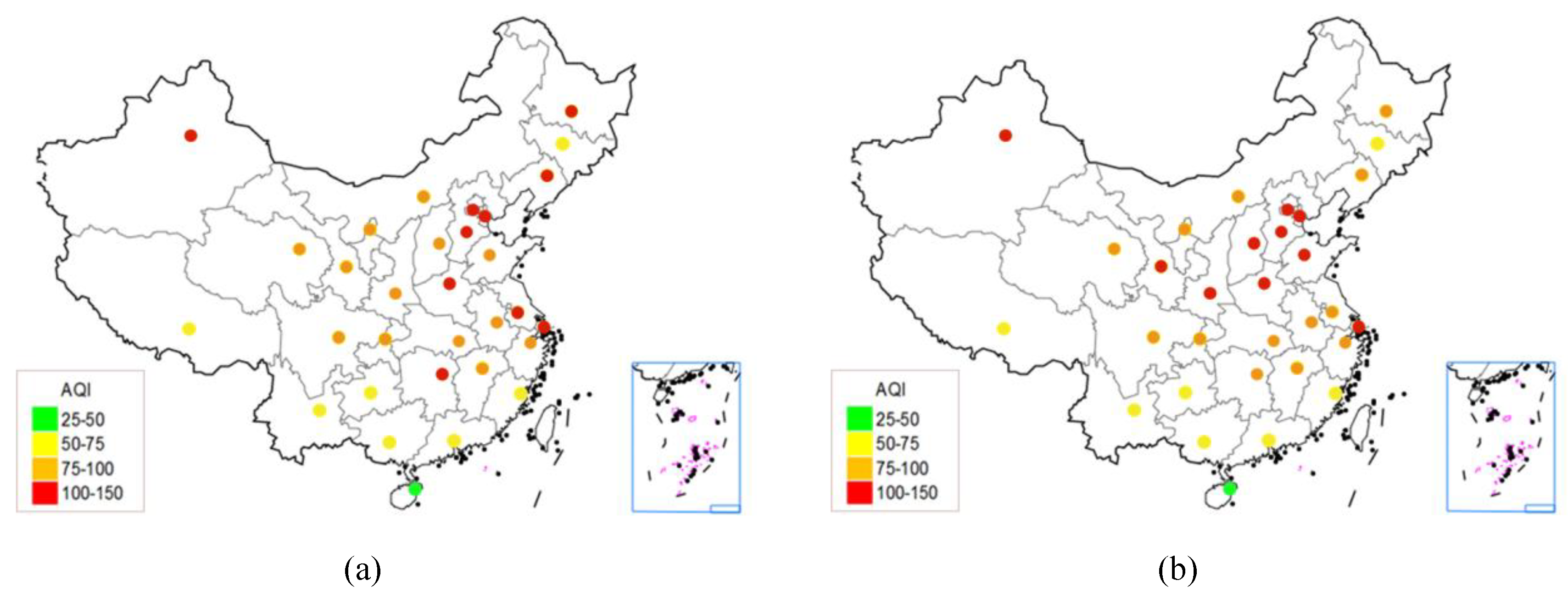
5.1. The Characteristics of Spatial Distribution of AQI

Due to the differences in natural conditions such as altitude, topography, sea and land location and climate, the air quality in China’s provincial capitals is better in the south than in the north, and better in the coastal areas than in the interior.

As shown in Figure 5, the air quality of coastal cities represented by Haikou and Fuzhou is better than others in 2018 because the southern part of China has a tropical or subtropical monsoon climate with relatively flat terrain, and the humid monsoon from the ocean in summer is conducive to the diffusion of urban pollutants. The air quality of cities in the high-altitude areas represented by Kunming and Lhasa also presents a better level. This is because there is little human activity in the high-altitude southwest, so the environment in this area has not been destroyed by human beings.

The cities with poor air quality are concentrated in the northeast, north and northwest of China. Northeast China, represented by Changchun, is China’s heavy industrial base and consumes a lot of coal and oil, so it has serious air pollution problems. In north China, represented by Shijiazhuang, there is a problem of low vegetation coverage, which cannot resist dust from northwest China. There is a potential relationship between the air quality and topography of the north China plain and the east Asian monsoon when westerly and southerly winds blow through the north and east of the region, leading to the accumulation of regional air pollutants [45]. Moreover, due to the low topography of north China, the diffusion conditions of air pollutants are poor. In north China, there is still the problem of large population density, and the rapid economic development and industrialization and urbanization process, so the damage to the environment is relatively serious. For the cities in northwest China, such as Urumqi, the distance from the sea is far, so water vapor is difficult to reach. Therefore, there is less precipitation, vegetation is scarce and the natural environment is harsh. All these reasons lead to poor air quality in northwest China.

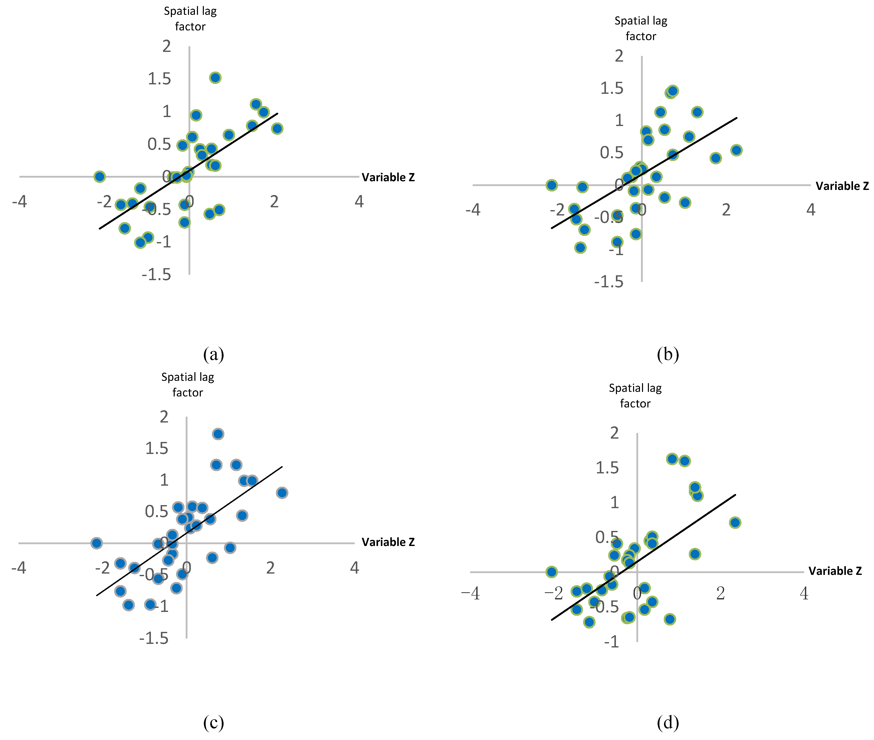
5.2. Spatial Correlation Analysis of AQI

We use the daily air quality index data of 31 provincial capitals from 2015 to 2018 to obtain the annual average value for each provincial capital, then calculate the global Moran index I and local Moran index I_i of each city every year. Further, we draw the scatter chart and LISA aggregation chart.

As shown in

Table 2. The global Moran index for 2015–2018.

Year	Moran’s I
2015	0.406
2016	0.458
2017	0.386
2018	0.384

, the Moran’s I from 2015 to 2018 is always positive, between 0.3 and 0.5. The value peaks at 0.458 in 2016 and falls to 0.384 in 2018. It indicates that there exists an obvious positive spatial correlation of China’s air quality. The air quality of a city is closely related to that of its neighboring cities.

In order to further study the local spatial autocorrelation of each region and explain the spatial aggregation model of different provinces and cities, we analyze the scatter diagram of the local Moran’s I_i.

The local spatial autocorrelation analysis is carried out through the Moran scatter plots, as indicated from Figure 6. The variable Z is the result of the standardization of AQI data, and the spatial lag factor $W_z$ is the vector of the weighted average of the neighbors around the observed value.AQI samples in China are mostly concentrated in the first quadrant (H-H) and the third quadrant (L-L), which indicates that most provinces in China are spatially dependent, while the rest are spatially heterogeneous.

H-H and L-L aggregation areas represent high (low) air quality in cities and high (low) air quality in surrounding cities. H-L and L-H aggregation areas stand for high (low) urban air quality surrounded by low (high) urban air quality, which means the AQI in the H-L aggregation area is high, but the AQI in surrounding cities is low. From Figure 7, the H-H aggregation areas in China are mainly distributed in cities in the central part of north China, such as Beijing, Shijiazhuang, Zhengzhou, Jinan and Taiyuan. The AQI index of cities in these areas is high, and that of surrounding cities is also high. Cities in China’s L-L aggregation areas are mainly distributed in parts of the northeast and the southern coastal areas, such as Changchun and Guangzhou. In addition, cities in the southwest plateau region, such as Kunming and Guiyang, are also located in the concentrated L-L area. The distribution characteristics are related to the fact that these cities are located in coastal areas, which is conducive to the diffusion of pollutants, or because of the low human activity in the plateau areas. There are few cities in the H-L and L-H aggregation areas, mainly concentrated in northwest China and the Yangtze River delta, such as Shanghai and Hangzhou.

From the above analysis, the urban air quality in China presents an obvious trend of aggregation. Therefore, the air pollution in the H-H aggregation area should be mainly treated to prevent its diffusion effect from further reducing the air quality in the surrounding cities and maintain the good air quality in the L-L aggregation area.

6. Spatio-Temporal Analysis of AQI

6.1. The Spatio-Temporal Characteristics of AQI

From Figure 8, the country’s air quality improved overall, from 2015 to 2018 The number of cities with poor air quality decreased significantly. Among them, the improvement of the air quality is most obvious in northeast China, such as Heilongjiang, Changchun and Shenyang, where the AQI index dropped by more than 30% from 2015 to 2018. The reason is that the state attaches great importance to revitalizing the old industrial base in northeast China, promoting industrial upgrading in this area, and developing high-tech industries with more environmental protection and lower consumption, so as to reduce the consumption of coal and oil, and improve the air quality gradually.

The air quality problem in Shijiazhuang has been high, with the AQI index over 100 from 2015 to 2018. This is because the Beijing–Tianjin–Hebei integration policy has relocated polluting enterprises from Beijing to Shijiazhuang, so the transformation and upgrading of polluting industries in Shijiazhuang cannot be completed in a short time. Besides, the pillar industry of Shijiazhuang is the high-pollution industry represented by steel manufacturing, which makes the air quality in Shijiazhuang unable to be improved effectively in recent years [46].

6.2. Spatio-Temporal Correlation Analysis of AQI

In

Table 3. Results of unit root test.

Method	Statistic	Prob.	Cross-Sections	Obs
Null: Unit root (assumes common unit root process)
Levin, Lin & Chu t	−20.4271	0.0000	31	90,209
Null: Unit root (assumes individual unit root process)
Im, Pesaran and Shin W-stat	−49.4335	0.0000	31	90,209
ADF-Fisher Chi-square	2360.07	0.0000	31	90,209
PP-Fisher Chi-square	6139.39	0.0000	31	90,489

, the p-values of the unit root tests are all less than 0.05; thus the null hypothesis is rejected. Within the 95% confidence level, the data do not have a unit root, so the sequence is stationary.

By the autocorrelation and partial correlation of the AQI values of the panel data in

Table 4. Autocorrelation(AC) and partial autocorrelation coefficients(PAC).

Autocorrelation	Partial Correlation		AC	PAC	Q-Stat	Prob
		1	0.809	0.809	1910.8	0.000
		2	0.686	0.093	3286.8	0.000
		3	0.599	0.060	4335.7	0.000
		4	0.533	0.043	5166.2	0.000
		5	0.481	0.036	5844.3	0.000
		6	0.447	0.051	6429.5	0.000
		7	0.421	0.041	6949.8	0.000
		8	0.400	0.033	7419.2	0.000
		9	0.363	-0.028	7804.9	0.000
		10	0.325	-0.014	8114.7	0.000
		11	0.311	-0.011	8532.5	0.000

, the autocorrelation (AC) and partial correlation (PAC) coefficients of the first eight stages of the lag period are all positive, while the PAC value of the ninth stage is negative, which indicates that the ninth stage of the lag period is not significant. Therefore, lag 8 is initially selected as the lag period of the model, and the model is tested by AIC and SC criteria. According to

Table 5. AIC/SC test results of lag period.

Lag	LogL	LR	FPE	AIC	SC	HQ
0	−20,829.83	NA	250,447.4	18.10676	18.11175	18.10858
1	−19,094.51	3466.109	55,612.60	16.60192	16.61689	16.60738
2	−18,989.31	209.9356	50,929.95	16.51396	16.53891	16.52306
3	−18,843.40	290.9283	45,019.99	16.39062	16.42555	16.40335
4	−18,651.82	381.6724	38,246.79	16.22757	16.27248	16.24394
5	−18,371.40	558.1535	30,078.22	15.98731	16.04220	16.00732
6	−18,001.50	735.6164	21,884.26	15.66928	15.73415	15.69293
7	−17,794.42	411.4690	18,343.02	15.49276	15.56761	15.52005
8	−17,421.06	741.2064	13,305.87	15.17171	15.25655	15.20264

, the AIC and SC values in the lag 8 attain a minimum, so the selection phase lag 8 is the best lag period.

After verifying the stationarity of the data, we need to select the type of panel data model. The selection of panel data models usually takes three forms: One is the pooled regression model. If, from the perspective of time, there is no significant difference between different individuals, from the view of the cross section, there is no significant difference between different cross sections, so the panel data can be directly mixed together and the parameters can be estimated by the ordinary least square method. One is the fixed effects regression model. If the model intercepts are different for different sections or different time series, the method of adding dummy variables to the model can be used to estimate the regression parameters. One is the random effects regression model. If the intercept term in the fixed effect model includes the average effect of the random error term of the section and the random error term of the time, and the two random error terms obey the normal distribution, then the fixed effect model becomes the random effect model. In the selection method of the panel data model form, we often use the $F$ test to decide whether to choose the mixed model or the fixed effect model, and then use the Hausman test to determine whether to establish the random effect model or the fixed effect model.

1. Mixed Effect Model

The results of the mixed effect model test are shown in

Table 6. Regression results of mixed effect model.

Variable	Coefficient	Std. Error	t-Statistic	Prob.
C	7.094672	0.187074	37.92441	0.0000
AQI(-1)	0.615542	0.003315	185.6643	0.0000
AQI(-2)	0.083921	0.003896	21.53917	0.0000
AQI(-3)	0.033636	0.003906	8.611525	0.0000
AQI(-4)	0.028408	0.003901	7.281393	0.0000
AQI(-5)	0.014703	0.003898	3.772412	0.0002
AQI(-6)	0.005298	0.003896	1.359862	0.1739
AQI(-7)	0.020360	0.003884	5.241592	0.0000
AQI(-8)	0.082582	0.003301	25.01919	0.0000

. For eight explanatory variables, it is found that the p-value of seven explanatory variables is less than 0.05. This indicates that under the confidence level of 95% most of these variables are significant. The regression results of the mixed effect model can be given by:

$$\begin{gathered} \widehat{\mathrm{AQI}}=0.62\mathrm{AQI}\left(-1\right)+0.08\mathrm{AQI}\left(-2\right)+0.03\mathrm{AQI}\left(-3\right)+0.02\mathrm{AQI}\left(-4\right)+0.01\mathrm{AQI}\left(-5\right)+ \\ 0.005\mathrm{AQI}\left(-6\right)+0.02\mathrm{AQI}\left(-7\right)+0.08\mathrm{AQI}\left(-8\right)+7.09, \end{gathered}$$

(7)

2. Individual Fixed Effect Model

The results of the individual fixed effect model test are shown in

Table 7. Regression results of individual fixed effect.

Variable	Coefficient	Std. Error	t-Statistic	Prob.
C	8.533101	0.198580	42.97050	0.0000
AQI(-1)	0.610168	0.003317	183.9326	0.0000
AQI(-2)	0.081511	0.003889	20.96025	0.0000
AQI(-3)	0.031613	0.003898	8.110045	0.0000
AQI(-4)	0.026505	0.003893	6.807735	0.0000
AQI(-5)	0.012783	0.003890	3.286554	0.0010
AQI(-6)	0.003301	0.003888	0.849068	0.3958
AQI(-7)	0.017961	0.003877	4.632740	0.0000
AQI(-8)	0.077332	0.003302	23.41681	0.0000
Fixed Effects (Cross)
BJ--C	2.068339
HK--C	−4.426904
CQ--C	−2.484907
FZ--C	−3.537358
WLMQ--C	3.239456
CD--C	−0.132934
NC--C	−1.155403
JN--C	4.455403
SH--C	−1.341894
LZ--C	2.365996
HF--C	0.321737
HHHT--C	1.017041
HEB--C	−2.088062
NN--C	−1.338221
TJ--C	2.047075
TY--C	4.706302
GZ--C	−2.110657
LS--C	−3.515151
KM--C	−1.849293
HZ--C	−2.079130
WH--C	0.349940
SY--C	−1.310719
SJZ--C	5.808012
XA--C	4.003164
GY--C	−2.614649
ZZ--C	3.647143
YC--C	2.355495
CC--C	−0.837571
CS--C	−0.675244
NJ--C	0.166678
XN--C	0.557123

. For first eight explanatory variables, the p-value of seven explanatory variables is less than 0.05, which also indicates that under the confidence level of 95%, most of these variables are significant. The regression results of the individual fixed effect model is given by:

$$\begin{gathered} \widehat{\mathrm{AQI}}=0.61\mathrm{AQI}\left(-1\right)+0.08\mathrm{AQI}\left(-2\right)+0.03\mathrm{AQI}\left(-3\right)+0.03\mathrm{AQI}\left(-4\right)+0.01\mathrm{AQI}\left(-5\right)+ \\ 0.003\mathrm{AQI}\left(-6\right)+0.02\mathrm{AQI}\left(-7\right)+0.08\mathrm{AQI}\left(-8\right)+8.53+2.06\mathrm{BJ}-4.42\mathrm{HK}\dots \dots +0.17\mathrm{NJ}+ \\ 0.56\mathrm{XN}, \end{gathered}$$

(8)

$\mathrm{BJ},\mathrm{HK},\mathrm{NJ},\mathrm{XN}$ are the regional dummy variables, which takes 1 if the current region is analyzed, otherwise it is 0. The coefficients of the dummy variables of each city are shown in Table 7.

3. Fixed Effect Test

The following are two hypotheses of the fixed effect test:

$H_0$: ${\gamma }_i=\gamma$, the intercept in different regions of the model is the same (mixed effect regression model should be established).

$H_1$: The intercept item${\gamma }_i$ is different in different regions in the model (individual fixed effect regression model should be established).

According to

Table 8. Results of fixed effect test.

Effects Test	Statistic	d.f.	Prob.
Cross-section F	15.003473	(30,90233)	0.0000
Cross-section Chi-square	449.179363	30	0.0000

, the p-value of this test is less than 0.05, so it is more reasonable to reject the null hypothesis $H_0$ and establish an individual fixed effect regression model.

4. Hausman Test

The following are two hypotheses tested by Hausman:

$H_0$: Individual effects are independent of regression variables (regression model of individual random effect should be established)

$H_1$: Individual effects are related to regression variables (regression model of individual fixed effect should be established)

According to

Table 9. Results of the Hausman test.

Test Summary	Chi-Sq. Statistic	Chi-Sq.d.f.	Prob.
Cross-section random	450.042246	8	0.0000

, the p-value of the Hausman test is less than 0.05, so it is more appropriate to reject the null hypothesis $H_0$ and establish an individual fixed effect model. Finally, the panel data model of fixed effect is established, as indicated by Equation (8). From Equation (8), the regression coefficients with the base period from the first stage to the eighth stage are 0.61, 0.08, 0.03, 0.01, 0.003, 0.02 and 0.08, respectively. This indicates that the AQI value of the first stage of lag has the greatest correlations with the value of the base stage, while from the second stage of lag to the eighth stage of lag are the second.

The reasons for the strongest correlations of AQI value in the first stage of lag and the second stage of lag is that the time distance between lags 1 and 2 is the closest to the base stage, and the factors affecting the AQI value do not change significantly within three hours and six hours, so the AQI value is highly correlated with the base stage. The correlation between the AQI value at base stage and the 8th stage lagging behind is significantly higher than that in the earlier stages. This is because the 8th stage lagging behind corresponds to 24 h away from the base stage, which means that the factors influencing the AQI value, such as natural conditions and human activities, are more similar to the base stage.

The absolute values of the correlation coefficients of the dummy variables for each region in Equation (8) reflect the degree of influence of the geographical location and surrounding cities on the air quality of the city. Shijiazhuang (SJZ) has the largest absolute value of dummy variable coefficient, which is 5.8. It shows that the air quality in SJZ is most influenced by its geographical location and the air quality of its surrounding cities. The reason is that SJZ is low-lying, which is not conducive to the diffusion of air pollutants, and the air quality in the surrounding areas is generally poor, which aggravates the air pollution problem in SJZ. Chengdu (CD) has the smallest absolute value of the dummy variable coefficient, which is −0.13. This is due to CD’s location in the Sichuan basin, which makes it more isolated from the surrounding area and less affected by the air quality of other cities.

To sum up, the following conclusions can be drawn in this part: The correlation coefficient between the air quality and its lag period is: A lag of 3 h > a lag of 6 h > a lag of 24 h. Moreover, due to the geographical location and the air quality of surrounding cities, the correlation coefficient of each dummy variable is significantly different.

7. Conclusions and Discussion

This paper studies the air quality of 31 provincial capitals in China from 2015 to 2018. From temporal, spatial and spatio-temporal analysis, the following conclusions are drawn:

7.1. The Characteristics of Air Quality of Chinese Cities Can Be Analyzed on Multiple Time Scales

The annual feature of China’s AQI is that China’s overall air quality improved from 2015 to 2018. This is closely related to the national and local governments vigorously carrying out pollution control work. The quarterly distribution of AQI is characterized by the best air quality in summer, followed by autumn, again in spring, and the worst air quality in winter. This result is consistent with previous studies. However, the difference between AQI indexes in spring, summer and autumn gradually decreases. This is because there is less precipitation in the winter and the air is dry. At the same time, the winter enters the heating period, and the pollution emissions increase, which aggravates air pollution. On the contrary, the increase of precipitation in summer, the increase of humidity and the increase of temperature are conducive to the dilution and pollution of pollutants. The diffusion has effectively improved air quality. Due to the continuous deepening of governance, the gap between seasons has gradually narrowed. At about 6 a.m. in a day, due to reduced human activity at night and reduced emissions of air pollutants, the AQI data reaches a lower level. There is a correlation effect between urban air quality and the lag period in China, and its correlation decreases with the increase of the time lag. This is because the various factors affecting the AQI index are gradually weakening, and the degree of correlation with air quality at a fixed time point is gradually decreasing. At the same time, there is a periodicity; the period is one day, which means the correlation at the same time point is strong every day. As shown in Table 1 above, the correlation coefficients of the AQI values and their lags in the twelve cities decrease with the increase of lags. The correlation coefficients of most cities such as Guangzhou, Kunming, and Changchun are in the 8th, the 16th and 24th periods showing a slight increase or inflection point and showing obvious periodicity.

7.2. The Air Quality of Provincial Capitals in China is Better in the South than in the North, and Better in the Coastal Areas than the Inland Areas

This is mainly related to factors such as climate type, topography and economic development level. Low pollutants are difficult to spread, and economic development and industrialization are fast, and environmental damage is more serious; southern coastal cities, represented by Fuzhou, are mostly tropical or subtropical monsoon climates, and the terrain is relatively flat. The humid monsoon from the ocean in summer is conducive to the diffusion of pollutants. There is an obvious positive spatial autocorrelation of air quality in China, and urban air quality in China shows an obvious tendency of aggregation. Cities with a high degree of air pollution will have a negative impact on the air quality of surrounding cities.

With this result, energy structures should be optimized and the proportion of green energy should be increased. China’s energy consumption structure is still given priority with coal; burning coal for heating or generating electricity from coal increases the concentration of air pollutants as it burns, so China needs to change the traditional energy consumption structure, reduce the coal consumption, raise the proportion of natural gas consumption and vigorously develop renewable energy sources such as wind, solar, geothermal energy. The government should take actions to alleviate the air pollution in some typical cities, as well as in winter [47]. It should promote the policy of "replacing coal with electricity" in northern China to reduce the use of coal for heating in winter; besides, promoting the popularity of new energy vehicles is an efficient way to control urban vehicle emissions and improve urban air quality. Through the survey of public attitudes towards air pollution control, it is found that respondents in China are very concerned about air pollution and believe that it is the duty of all citizens to improve air quality. When necessary, they are willing to use new energy vehicles to replace traditional energy vehicles [48].

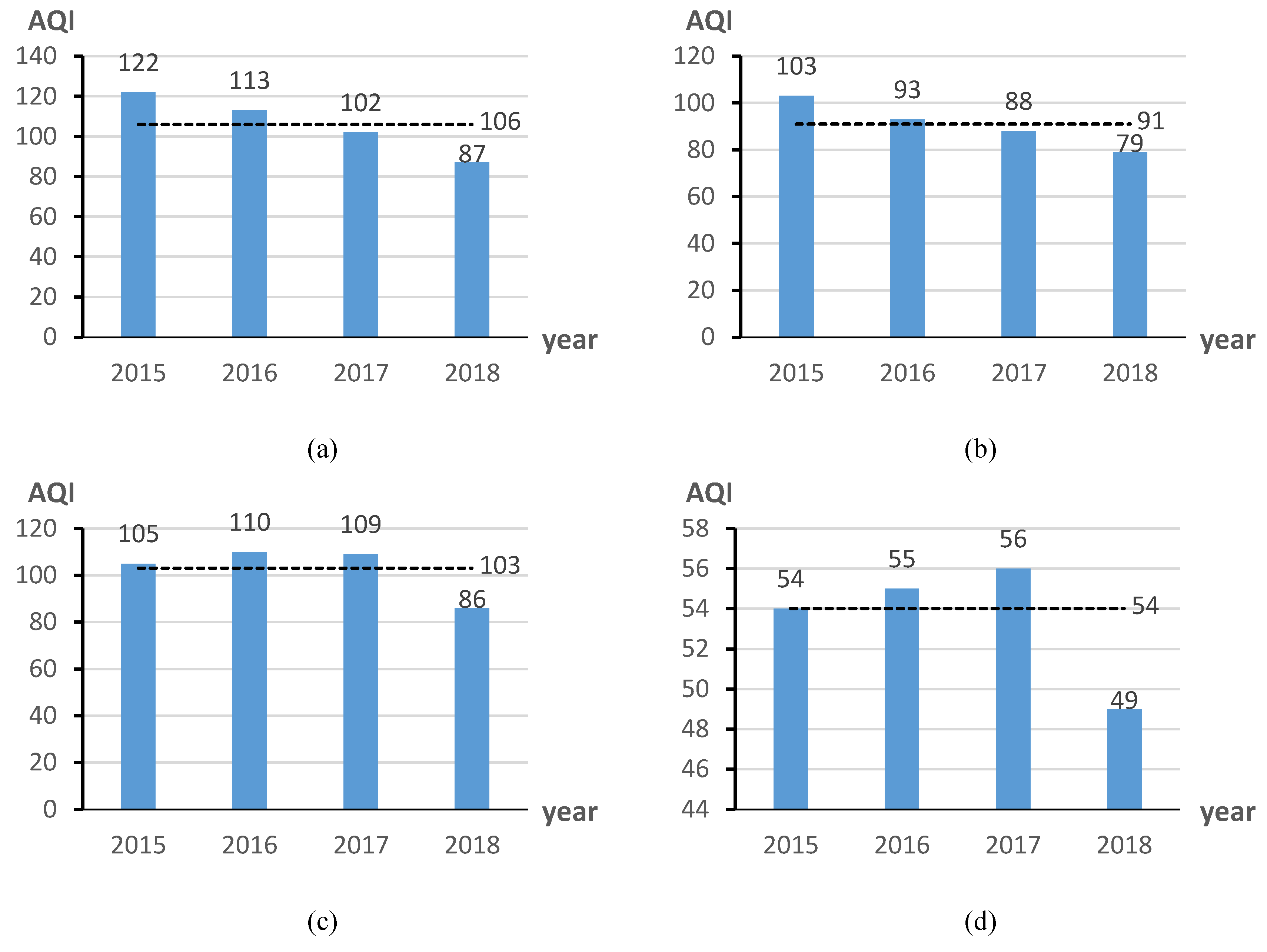
7.3. The Air Quality of Chinese Cities Has Improved From 2015 to 2018.

The number of provinces with poor air quality decreased significantly, while the number of provinces with good air quality increased significantly compared with 2015. The overall conclusion is consistent with the findings of other authors. Northeast China, such as Heilongjiang, Changchun and Shenyang, has seen the most significant improvement in air quality, while Shijiazhuang still has a serious air pollution problem. The reason is that the country attaches importance to revitalizing the old industrial bases in the northeast, promotes industrial upgrading in the three eastern provinces, develops more environmentally friendly and low-consumption high-tech industries and reduces the consumption of coal and oil. The air quality has gradually improved. On the other hand, due to the Beijing–Tianjin–Hebei integration policy, Beijing’s polluting enterprises have been relocated to Shijiazhuang, so the transformation and upgrading of high-pollution industries in Shijiazhuang cannot be completed in a short time.

7.4. The Relationship between the Correlation Coefficient of Chinese Urban Air Quality Has a Lag Period

The lag period is as follows: A lag of 3 h > a lag of 6 h > a lag of 24 h. Moreover, due to the relative location of different regions and the influence of climate and other factors, the absolute values of the correlation coefficients of dummy variables in different regions are greatly different. The result suggests that there is a strong correlation between air quality in different provinces in China, especially in north China including Beijing. Cities in north China need to work together to tackle air pollution, which is a regional problem rather than a local one [49]. We believe that effective air pollution control policies should be regional, but in order to address air pollution more effectively, cross-border cooperation between regional and local governments is essential [50]. Controlling air pollution problems, therefore, should involve implementing a regional combination, breaking the limitation of administrative regions and establishing a regional air pollution control management agency. It is short sighted to deal with the air pollution problem in a region at the cost of the environmental benefits of the surrounding region, so it is our duty to achieve coordinated regional air pollution control.

While this study has successfully explored the correlation between the air quality in Chinese cities and its lag period from the perspective of space and time, there are still deficiencies, which can be considered in future research. Due to the lack of concentration data of the study on factors leading to air pollution, the close relationship between the air quality and human factors as well as natural factors such as the temperature, vegetation and terrain cannot be highlighted, so the conclusion obtained should be cautious. Wang et al. [51] studied the spatial and temporal patterns and dynamics of urban aerosols using AOD data in phoenix and Los Angeles. The correlation analysis shows that, compared with the urban land use and the vegetation, topography is the main factor affecting the spatial pattern of AOD. The impact of human factors such as urbanization on air pollution varies with the existing landscape, which significantly alleviates aerosol concentrations. In addition, plants release fine aerosols, which can reduce air pollution. Generally speaking, temporal variation characteristics and regional differences in air pollutant concentration are the result of the comprehensive effects of meteorological conditions, landform, vegetation coverage, human activities and socio-economic development level. The influence of natural factors and anthropogenic factors on urban air quality distribution needs to be further studied.

References

1. Xie, R.; Zhao, G.; Zhu, B.Z. Examining the Factors Affecting Air Pollution Emission Growth in China. Environ. Model. Assess. 2018, 23, 389–400. [Google Scholar] [CrossRef]
2. He, J.X.; Liu, H.M.; Salvo, A. Severe Air Pollution and Labor Productivity: Evidence from Industrial Towns in China. Am. Econ. J. Appl. Econ. 2019, 11, 173–201. [Google Scholar] [CrossRef] [Green Version]
3. Rui, L.; Wang, Z.Z.; Cui, L.L. Air pollution characteristics in China during 2015–2016: Spatiotemporal variations and key meteorological factors. Sci. Total Environ. 2019, 658, 902–915. [Google Scholar]
4. Xu, Y.T.; Liu, X.Y.; Wang, Z.B. Temporal and spatial distribution characteristics of urban air quality in China based on AQI index. J. Guangxi Norm. Univ. Nat. Sci. Ed. 2019, 37, 187–196. [Google Scholar]
5. Xiao, Y.; Tian, Y.Z.; Xu, W.X.; Wu, J.J.; Tian, L. Temporal and spatial distribution characteristics of air quality in China in recent 10 years. J. Eco-Environ. 2017, 26, 243–252. [Google Scholar]
6. Guo, H.; Gu, X.; Ma, G. Spatial and temporal variations of air quality and six air pollutants in China during 2015–2017. Sci. Rep. 2019, 9. [Google Scholar] [CrossRef] [Green Version]
7. Xia, X.; Qi, Q.; Liang, H.; Zhang, A.; Jiang, L.; Ye, Y.; Liu, C.; Huang, Y. Pattern of Spatial Distribution and Temporal Variation of Atmospheric Pollutants during 2013 in Shenzhen. China ISPRS Int. J. Geo-Inf. 2017, 6, 2. [Google Scholar] [CrossRef]
8. Zhan, D.S.; Kwan, M.P.; Zhang, W.Z. The driving factors of air quality index in China. J. Clean. Prod. 2018, 197, 1342–1351. [Google Scholar] [CrossRef]
9. Tian, Y.L.; Jiang, Y.J.; Liu, Q.; Xu, D.X.; Zhao, S.D.; He, L.H.; Liu, H.J.; Xu, H. Temporal and spatial trends in air quality in Beijing. Landsc. Urban Plan. 2019, 185, 35–43. [Google Scholar] [CrossRef]
10. He, J.J.; Gong, S.L.; Yu, Y. Air pollution characteristics and their relation to meteorological conditions during 2014–2015 in major Chinese cities. Environ. Pollut. 2017, 223, 484–496. [Google Scholar] [CrossRef]
11. Tao, Y.T.; Wu, Y.Q. Analysis of the spatio-temporal pattern of national air quality based on Moran ‘I index. J. Nat. Disasters 2018, 27, 107–113. [Google Scholar]
12. He, Z.G.; Han, S.M.; Cui, D.Y. Discussion on the statistics of spatial autocorrelation analysis. Chin. J. Schistosomiasis Control 2008, 20, 315–318. [Google Scholar]
13. Fang, C.; Liu, H.; Li, G.; Sun, D.; Miao, Z. Estimating the Impact of Urbanization on Air Quality in China Using Spatial Regression Models. Sustainability 2015, 7, 15570–15592. [Google Scholar] [CrossRef] [Green Version]
14. He, R.R.; Zhu, L.B.; Zhou, K.S. Spatial autocorrelation analysis of air quality index (AQI) in eastern China based on residuals of time series models. Acta Sci. Circumstantiae 2017, 37, 2459–2467. [Google Scholar]
15. Dadhich, A.P.; Goyal, R.; Dadhich, P.N. Assessment of spatio-temporal variations in air quality of Jaipur city, Rajasthan, India. Egypt. J. Remote Sens. Space Sci. 2018, 21, 173–181. [Google Scholar] [CrossRef]
16. Liu, H.J.; Du, G.J. Spatial pattern and distribution of air pollution in Chinese cities: An empirical study based on 161 AQI and 6 sub-pollutants. Econ. Geogr. 2016, 36, 33–38. [Google Scholar]
17. Liu, L.; Yang, X.; Wang, M.; Long, Y.; Shen, H.; Nie, Y.; Chen, L.; Guo, H.; Jia, F.; Nelson, J.; et al. Climate Change, Air Quality and Urban Health: Evidence from Urban Air Quality Surveillance System in 161 Cities of China 2014. J. Geosci. Environ. Prot. 2018, 6, 117–130. [Google Scholar] [CrossRef] [Green Version]
18. Zhu, J.; Zhang, J.; Fu, Y.P. Spatial econometric analysis of air quality in provinces in China. Sci. Technol. Bull. 2018, 34, 256–260. [Google Scholar]
19. Xu, W.; Tian, Y.; Liu, Y.; Zhao, B.; Liu, Y.; Zhang, X. Understanding the Spatio-Temporal Patterns and Influential Factors on Air Quality Index: The Case of North China. Int. J. Environ. Res. Public Health 2019, 16, 2820. [Google Scholar] [CrossRef] [Green Version]
20. Huang, W.; Wang, H.; Wei, Y. Endogenous or Exogenous? Examining Trans-Boundary Air Pollution by Using the Air Quality Index (AQI): A Case Study of 30 Provinces and Autonomous Regions in China. Sustainability 2018, 10, 4220. [Google Scholar] [CrossRef] [Green Version]
21. Li, X.F.; Zhang, M.J.; Wang, S.J. Analysis of the characteristics and influencing factors of China’s air pollution index. Environ. Sci. 2012, 33, 1936–1943. [Google Scholar]
22. Pu, H.; Luo, K.; Wang, P. Spatial variation of air quality index and urban driving factors linkages: Evidence from Chinese cities. Environ. Sci. Pollut. Res. 2017, 24, 4457. [Google Scholar] [CrossRef]
23. Zhao, S.P.; Yu, Y.; Yin, D.Y.; He, J.J.; Liu, N.; Qu, J.J.; Xiao, J.H. Annual and diurnal variations of gaseous and particulate pollutants in 31 provincial capital cities based on in situ air quality monitoring data from China National Environmental Monitoring Center. Environ. Int. 2016, 86, 92–106. [Google Scholar] [CrossRef]
24. Xu, L.; Zhou, J.X.; Guo, Y. Spatiotemporal pattern of air quality index and its associated factors in 31 Chinese provincial capital cities. Air Qual. Atmos. Health 2017, 10, 601. [Google Scholar] [CrossRef]
25. Liu, Y.P.; Wu, J.G.; Yu, D.Y. Characterizing spatiotemporal patterns of air pollution in China: A multiscale landscape approach. Ecol. Indic. 2017, 76, 344–356. [Google Scholar] [CrossRef] [Green Version]
26. Luo, G.L. Cluster analysis of air quality panel data of major cities in China. Mod. Bus. Ind. 2014, 07, 12–13. [Google Scholar]
27. Boyce, M.S.; Pitt, J.; Northrup, J.M.; Morehouse, A.T.; Knopff, K.H.; Cristescu, B.; Stenhouse, G.B. Temporal autocorrelation functions for movement rates from global positioning system radiotelemetry data. Philos. Trans. R. Soc. B Biol. Sci. 2010, 365, 2213–2219. [Google Scholar] [CrossRef] [Green Version]
28. Liu, J.; Wang, H.W.; Yang, J. Research on Influencing Factors of Air Pollution in China—Analysis Based on China’s Urban Dynamic Spatial Panel Model. J. Hohai Univ. 2017, 19, 61–67. [Google Scholar]
29. Modarres, R.; Dehkordi, A.K. Daily air pollution time series analysis of Isfahan City. Int. J. Environ. Sci. Technol. 2005, 2, 259–267. [Google Scholar] [CrossRef] [Green Version]
30. Farah, W.; Nakhlé, M.M.; Abboud, M. Time series analysis of air pollutants in Beirut. Lebanon. Environ. Monit. Assess. 2014, 186, 8203–8213. [Google Scholar] [CrossRef]
31. Klemm, O.; Lange, H. Trends of air pollution in the Fichtelgebirge Mountains Bavaria. Environ. Sci. Poll. Res. 1999, 6, 193–199. [Google Scholar] [CrossRef] [PubMed]
32. Qiang, S. A note on fuzzy time series model selection with sample autocorrelation functions. Cybern. Syst. 2010, 93–107. [Google Scholar]
33. Getis, A. Spatial Autocorrelation. Handbook of Applied Spatial Analysis; Springer: Berlin/Heidelberg, Germany, 2010; pp. 255–278. [Google Scholar]
34. Tiefelsdorf, M. The saddlepoint approximation of Moran’s I’s and local Moran’s Ii’s reference distributions and their numerical evaluation. Geogr. Anal. 2002, 34, 187–206. [Google Scholar] [CrossRef]
35. Elhorst, J.P. Spatial Panel Data Models. In Spatial Econometrics; Springer: Berlin/Heidelberg, Germany, 2014; pp. 37–93. [Google Scholar] [CrossRef]
36. Fischer, M.M.; Scherngell, T.; Reismann, M. Knowledge Spillovers and Total Factor Productivity: Evidence Using a Spatial Panel Data Model. Geogr. Anal. 2009, 41, 204–220. [Google Scholar] [CrossRef] [Green Version]
37. Elhorst, J.P. Specification and Estimation of Spatial Panel Data Models. Int. Reg. Sci. Rev. 2003, 26, 244–268. [Google Scholar] [CrossRef]
38. Baltagi, B.H.; Song, S.H.; Koh, W. Testing panel data regression models with spatial error correlation. J. Econ. 2003, 117, 123–150. [Google Scholar] [CrossRef]
39. Halaby, C.N. Panel Models in Sociological Research: Theory into Practice. Ann. Rev. Sociol. 2004, 30, 507–544. [Google Scholar] [CrossRef]
40. Amini, S.; Delgado, M.; Henderson, D.; Parmeter, C. Fixed vs Random: The Hausman Test Four Decades Later. Adv. Econ. 2012, 29, 479–513. [Google Scholar]
41. Mutl, J.; Pfaffermayr, M. The Hausman test in a Cliff and Ord panel model. Econ. J. 2011, 14, 48–76. [Google Scholar] [CrossRef]
42. Li, H.; You, S.J.; Zhang, H.; Zheng, W.D.; Zheng, X.J.; Jia, J.; Ye, T.Z.; Zou, L.J. Modelling of AQI related to building space heating energy demand based on big data analytics. Appl. Energy 2017, 203, 57–71. [Google Scholar] [CrossRef]
43. Zhang, Y.; Ding, A.J.; Mao, H.T.; Nie, W.; Zhou, D.R.; Liu, L.X.; Huang, X.; Fu, C.B. Impact of synoptic weather patterns and inter-decadal climate variability on air quality in the North China Plain during 1980–2013. Atmos. Environ. 2016, 124, 119–128. [Google Scholar] [CrossRef]
44. Song, J.; Wang, Z.H.; Wang, C. Biospheric and anthropogenic contributors to atmospheric CO2 variability in a residential neighborhood of Phoenix, Arizona. J. Geophys. Res. Atmos. 2017, 122, 3317–3329. [Google Scholar] [CrossRef]
45. Wang, J.; Yang, P.; Zhang, X.; Zhao, Z.; Wei, F.; Zhang, J. A Review of Air Pollution and Control in Hebei Province, China. Open J. Air Pollut. 2013, 2, 47–55. [Google Scholar] [CrossRef] [Green Version]
46. Wang, Z.; Zhao, J.; Xu, J.; Jia, M.; Li, H.; Wang, S. Influence of Straw Burning on Urban Air Pollutant Concentrations in Northeast China. Int. J. Environ. Res. Public Health 2019, 16, 1379. [Google Scholar] [CrossRef] [PubMed] [Green Version]
47. Bao, J.; Yang, X.; Zhao, Z.; Wang, Z.; Yu, C.; Li, X. The Spatio-Temporal Characteristics of Air Pollution in China from 2001–2014. Int. J. Environ. Res. Public Health 2015, 12, 15875–15887. [Google Scholar] [CrossRef] [PubMed] [Green Version]
48. Liu, H.; Kobernus, M.; Liu, H. Public Perception Survey Study on Air Quality Issues in Wuhan, China. J. Environ. Prot. 2017, 8, 1194–1218. [Google Scholar] [CrossRef] [Green Version]
49. Chen, W.; Tang, H.Z.; Zhao, H.M. Urban air quality evaluations under two versions of the national ambient air quality standards of China. Atmos. Pollut. Res. 2016, 7, 49–57. [Google Scholar] [CrossRef]
50. Li, Q.; Wang, E.; Zhang, T. Spatial and Temporal Patterns of Air Pollution in Chinese Cities. Water Air Soil Pollut. 2017, 228, 92. [Google Scholar] [CrossRef]
51. Wang, C.; Wang, C.; Myint, S.W.; Wang, Z.H. Landscape determinants of spatio-temporal patterns of aerosol optical depth in the two most polluted metropolitans in the United States. Sci. Total Environ. 2017, 609, 1556–1565. [Google Scholar] [CrossRef]
Figure 1. (a) The average air quality index (AQI) in Beijing from 2015 to 2018. (b) The average AQI in Wuhan from 2015 to 2018. (c) The average AQI in Urumqi from 2015 to 2018. (d) The average AQI in Kunming from 2015 to 2018.
Sustainability 12 02486 g001
Figure 2. (a) Quarterly average of Shenyang AQI from 2015 to 2018. (b) Quarterly average of Nanchang AQI from 2015 to 2018. (c) Quarterly average of Lanzhou AQI from 2015 to 2018. (d) Quarterly average of Guiyang AQI from 2015 to 2018.
Sustainability 12 02486 g002aSustainability 12 02486 g002b
Figure 3. (a) Mean daily AQI of Shanghai in 2018. (b) Mean daily AQI of Taiyuan in 2018. (c) Mean daily AQI of Harbin in 2018. (d) Mean daily AQI of Changchun in 2018.
Sustainability 12 02486 g003
Figure 4. (a) Correlation coefficient between Beijing AQI and its lag in 2018. (b) Correlation coefficient between Hohhot AQI and its lag in 2018. (c) Correlation coefficient between Hangzhou AQI and its lag in 2018. (d) Correlation coefficient between Nanning AQI and its lag in 2018.
Sustainability 12 02486 g004aSustainability 12 02486 g004b
Figure 5. The distribution of AQI of cities in China in 2018.
Sustainability 12 02486 g005
Figure 6. (a) Moran scatter chart of annual mean value of AQI in 2015. (b) Moran scatter chart of annual mean value of AQI in 2016. (c) Moran scatter chart of annual mean value of AQI in 2017. (d) Moran scatter chart of annual mean value of AQI in 2018.
Sustainability 12 02486 g006
Figure 7. LISA agglomeration diagram of air quality in Chinese cities in 2018.
Sustainability 12 02486 g007
Figure 8. (a) Annual Average AQI Distribution Map of China in 2015. (b) Annual Average AQI Distribution Map of China in 2016. (c) Annual Average AQI Distribution Map of China in 2017. (d) Annual Average AQI Distribution Map of China in 2018.
Sustainability 12 02486 g008aSustainability 12 02486 g008b