Article

Microsimulation of Residential Activity for Alternative Urban Development Scenarios: A Case Study on Brussels and Flemish Brabant

1
Cartography and GIS Research Group, Vrije Universiteit Brussel, 1050 Brussels, Belgium
2
Building, Architecture and Town Planning, Université Libre de Bruxelles, 1050 Brussels, Belgium
*
Author to whom correspondence should be addressed.
Sustainability 2020, 12(6), 2370; https://doi.org/10.3390/su12062370
Submission received: 3 February 2020 / Revised: 2 March 2020 / Accepted: 13 March 2020 / Published: 18 March 2020
(This article belongs to the Special Issue Urban Sprawl and Sustainability II)

Abstract

:
The historically rooted suburbanization of Flanders and the Brussels Capital Region (BCR) in Belgium has resulted in severe urban sprawl, traffic congestion, natural land degradation and many related problems. Recent policy proposals put forward by the two regions aim for more compact urban development in well-serviced areas. Yet, it is unclear how these proposed policies may impact residential dynamics over the coming decades. To address this issue, we developed a Residential Microsimulation (RM) framework that spatially refines coarse-scale demographic projections at the district level to the level of census tracts. The validation of simulated changes from 2001 to 2011 reveals that the proposed framework succeeds in modelling historic trends and clearly outperforms a random model. To support simulation from 2011 to 2040, two alternative urban development scenarios are defined. The Business As Usual (BAU) scenario essentially represents a continuation of urban sprawl development, whereas the Sustainable Development (SUS) scenario strives for higher-density development around strategic well-serviced nodes in line with proposed policies. This study demonstrates how residential microsimulation supported by scenario analysis can play a constructive role in urban policy design and evaluation.

1. Introduction

Flanders, the northern part of Belgium, is among the regions that are most strongly characterized by urban sprawl in Europe [1]. This has contributed to an unsustainable mobility model that is excessively dependent on private car use [2]. Predictably, Flemish roads are also among the most congested in Europe [3,4]. Urban sprawl and road congestion contribute significantly to negative environmental and health impacts [5,6], greenhouse gas emission [7], landscape and ecosystem degradation [8,9,10] and economic losses [3,11]. The problematic spatial organization of Flanders has a long history, going back to nineteenth-century industrialization, and is aggravated by poor coordination between the political regions of Belgium, which transitioned from a unitary to a federal governance model in the 1970s [12,13]. Both Flanders and the Brussels Capital Region (BCR) have recently pointed out the need for more sustainable urban development strategies [14,15]. Higher-density development around well-serviced urban hubs, decreasing private car use and improving interregional cooperation are important features of the strategies proposed in the two regions. What is lacking, however, is an understanding of how strategic plans may affect residential dynamics, i.e., where different types of households will end up living over time. Having spatially detailed knowledge on expected demographic changes is of considerable importance for regional and municipal governance, to better plan its infrastructure and services, or to adjust strategies should they potentially yield undesirable results. In this research, we address this topic by means of Residential Microsimulation (RM) and scenario analysis.
RM is a modelling approach that considers residential activity of individuals and households [16]. If the microsimulation has a path-dependent temporal dimension and covers geographic units, it is said to be dynamic and spatial [17,18]. The idea of microsimulation has been around since the 1950s [19], yet it expanded into a research field mainly from the 1970s onward, driven by developments in computational capacity [16,18,20]. RM draws heavily on residential location choice modelling, which can be described as a behavioral modelling approach that attempts to quantify the process of deciding one’s place of residence. Although several methods are suited to performing this type of analysis [21], discrete choice modelling based on the random utility framework is widely used [22,23]. Important examples of spatial dynamic RM applications include UrbanSim [24,25,26], ILUTE (Integrated Land Use Transport Environment) [27,28] and ILUMASS (Integrated Land Use Modelling and Transportation System Simulation) [29]. RM can be used to spatially disaggregate regional demographic projections to smaller geographic units [30,31]. Another feature of RM is its ability to spatiotemporally assess changing relations between various aspects of the urban environment. By doing so, it can yield emerging behavior, i.e., outcomes that are difficult to predict based solely on an understanding of the underlying system at one point in time. Hence, RM is considered to be a useful tool to support integrated urban modelling or to evaluate policy [32]. Spatial dynamic RM is often used to investigate the effects of economic or social policy on residential activity, particularly in relation to demography [33,34], taxation [35], the housing market [36], public health [37,38] and transport [27,28]. RM rests on inductive logic, using regression-based or other data-driven algorithms, and typically involves large numbers of choice agents and location alternatives. Consequently, RM can be computational and data intensive, requiring considerable information on the involved population and environment [16,39,40].
Spatial dynamic RM is often accompanied by one or more scenario to support simulation into the future. A scenario is a timeline entailing assumptions, constraints and events, designed according to a narrative of what the future may look like [41,42]. Scenarios are thus idealized representations of the future, used to deal with the complexity and uncertainty of modelling phenomena beyond the present [43]. They are by definition subjective, and should not be interpreted as predictions per se, but more as complementary visions. As such, scenarios can be used to set the topic of discussion or to compare the expected outcomes of strategies and policies [44]. Originating from military and corporate backgrounds, scenario planning has only slowly found its way into science, in part due to its somewhat ambiguous conceptual foundation [42]. Over the past decades, several authors have contributed to creating a stronger theoretical and practical basis for scenario development and its application [42,43,45,46]. Among these authors, it is generally agreed that scenarios should be relevant, plausible, consistent and unique. Scenarios should, furthermore, have clearly identified topics, stakeholders, spatiotemporal scope and drivers of changes. If scenarios are used to perform quantitative analyses, suitable metrics must also be defined. Scenario analysis is increasingly used in sustainability research to explore alternative development pathways [47,48,49].
Some studies combine RM and scenario analysis to answer questions related to (hypothetic) policies [24,34,50,51], e.g., “what are the expected impacts of policy measures X and Y on residential dynamics, and how do they compare?”. So far, however, few studies apply RM in the context of assessing impacts of spatial planning scenarios, particularly with regard to urban sprawl versus more sustainable forms of urban development. In [52], RM is used to project the future urban development of Montreal for three urban planning scenarios depicting alternative assumptions with regard to the evolution of housing stock distribution. Another Canadian study on the city of Hamilton [53] simulates residential relocation for six urbanization scenarios representing varying degrees of urban sprawl and assesses the impact of these scenarios on transport-related emission and energy consumption. In a similar study on Beijing, [54] use RM and urban densification scenarios to explore future transport emmission up to 2030. An American study by [55] simulates residential and firm locations in Austin (Texas) under, among others, an urban growth boundary scenario, with the intent to also forecast greenhouse gas emission. The urban planning scenarios in the above studies, while useful in their respective research contexts, are quite vaguely defined and lack a more explicit spatial basis to support their validity with regard to spatial policy and its associated tools, i.e., legislated regional strategies, zoning restrictions, historic/ecologically protected areas and use of land registry data, etc.
The overarching objective of this research is to demonstrate that spatial dynamic RM supported by spatially explicit scenario analysis can contribute to a better informed discussion on urban development policy. To do so, we address the so far underexploited potential of RM for exploring sustainable urban development pathways. Countering urban sprawl in Brussels and Flanders is a particularly relevant case to illustrate this point. The objectives of this study are: (1) developing and presenting a spatial dynamic RM framework; (2) testing and validating this simulation framework for a timeframe covering the last two Belgian Censuses; (3) defining two alternative urban development scenarios for our case study, using all the relevant spatial information at our disposal; and (4) applying the RM framework to simulate residential dynamics up to 2040 for both scenarios. With this work, we try to contribute to narrowing the gap that is still present between the fields of spatial modelling and strategic level spatial planning.
The rest of this paper is structured as follows. Firstly, the study area of this research is delineated. Secondly, we give an overview of the used datasets. Thirdly, the Methods section covers the microsimulation framework, validation strategy and scenario analysis. Finally, our results are presented and discussed.

2. Study Area

The study area of this research entails three districts located in the centre of Belgium: the BCR, Halle-Vilvoorde and Leuven (Figure 1). Together, the districts of Halle-Vilvoorde and Leuven form the province of Flemish Brabant. The study area covers two political regions, the BCR and Flanders, and 84 municipalities. While the BCR is quite densely built-up in accordance with its economic activities, the districts of Halle-Vilvoorde and Leuven are characterized by extensive urban sprawl. In 2011, the year of the last Census, 980,701 households resided in the three districts of the study area and 1,084,039 people were employed in it [56,57]. Despite the BCR being the largest employment centre in the country, it also has the highest regional unemployment rate [58], as much of its workforce comes from Flanders and Wallonia. The pervasiveness of private car commuting combined with the poorly designed road infrastructure in and around the BCR frequently results in extreme road congestion. According to the TomTom [59] and INRIX [60] congestion indices, Brussels is among the most congested cities in the world, despite being a relatively small city. In addition to these challenges, Brussels and its urban periphery are projected to be among the fastest growing areas of the country in terms of residential [61] and economic activity [56].

3. Data

Table 1 shows an exhaustive list of the data sources used in this research. Besides the Census and relocation data, which are privacy sensitive, most of the other datasets used are open data that are freely available for download on the web portals of their respective data providers. The first four rows in Table 1 are the main datasets for this study. A complete list of households residing in the study area, with observed locations on ward level in 2001 and 2011, was obtained from the last two Censuses. The Census data also provides certain characteristics of the Reference Person (RP) of each household. Demographic trends on a district level were provided by HPROM (Household Projection Model) projections produced by the Federal Planning Bureau. Employment potential was derived by combining multiple sources. The locations of all company establishments in Belgium were identified by geocoding the Crossroads Bank for Enterprises database using the Central Reference Address Database. The number of employees per establishment was estimated using additional data from the Federal Public Service (FPS) Mobility and Transport and the National Social Security Office. Residential relocation frequency was quantified by means of a microsample made available for this research by Statistics Belgium. The microsample covers a randomly drawn 20% sample of all Belgian households with the corresponding sector of residence at the start of 2003 and 2004. It is considered representative of household movements taking place within the Belgian territory.
Given the strong relation between public/private transport and urban sprawl, information on the availability and proximity of transport infrastructure and its use was included in the modelling. A zoning map showing areas with good and poor access to public transport and services was derived from a policy support study on densification-oriented urban development for Flanders [62]. This map constitutes one of the key inputs in the scenario definition. To address the socio-economic realities faced by households relating to housing costs and social housing [63,64,65], use was made of data provided by Statistics Belgium, the Brussels Institute for Statistics and Analysis and the Flemish Society for Social Housing.
To define urban development scenarios in a spatially explicit fashion, a spatial analysis of zoning, parcel and building data proved essential to quantify feasable evolutions of housing stock distributions. Because urban development does not occur in a vacuum, it is also important to address additional geographic constraints. Hence, we included information on cultural heritage and ecologically protected areas in the scenario definition. Knowing that flooding is a frequent occurrence in Brussels and Flanders [66], and that historically many flood-prone areas have been developed despite this knowledge [67], the choice was made to integrate flood-prone areas in the scenario analysis.

4. Methods

4.1. Overview Research

For this research, we developed a spatiotemporal microsimulation framework and applied it to simulate residential dynamics in the BCR and the two surrounding Flemish districts. In our approach, we used HPROM household projections [61,68,69] for different household types, which are defined on a district level as an exogenous demographic model. Relocation behavior was modelled by means of a microsample made available by Statistics Belgium. Simulation was performed by letting households choose from individual dwellings defined on a statistical ward level, the finest scale on which statistics are published in Belgium. As such, our microsimulation constitutes a spatial disaggregation of the HPROM projections from the district to statistical ward level. We first performed RM between 2001 and 2011, the years of the last two Censuses, to assess simulation accuracy. Scenario analysis was then performed to simulate residential dynamics for the period 2011-2040. To do so, we defined two scenarios representing alternative urban planning policies with regard to residential development. The first scenario is called Business As Usual (BAU) and is based on current planning practice that has led to extensive urban sprawl. The second scenario is called Sustainable Development (SUS) and is based on recently proposed spatial planning strategies for Flanders and the BCR, aiming at denser urban development in well-serviced areas. Both scenarios were defined in a spatially explicit fashion, using land registry, zoning and other relevant spatial data. Essentially, the scenarios quantify how housing stock may evolve over time, using their respective underlying rationales.
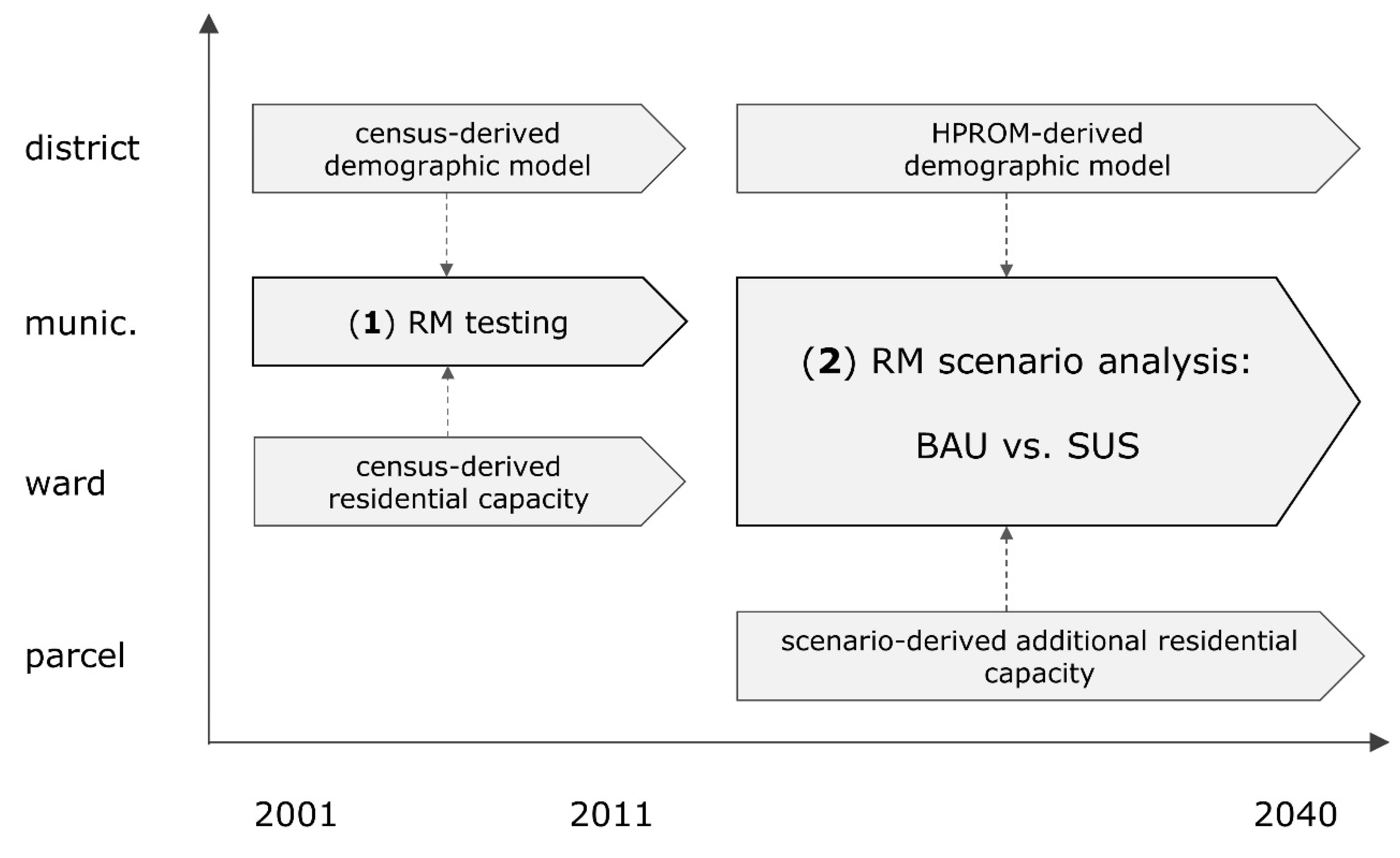
Figure 2 shows a time-scale perspective overview of the two residential microsimulation experiments and the supportive analyses performed for this research. The first part of the research covered testing the proposed RM framework between 2001 and 2011. To do so, we drew on Census data, particularly the locations of each household in 2001 and 2011, as well as the evolution of the housing stock between those years. The former served as a driver of change in residential activity. The latter provided us with constraints, i.e., the number of dwellings available per ward. Simulation was performed on the ward level, yet an accuracy assessment was performed on the more spatially aggregated level of the municipality. In a second phase, we performed scenario analysis between 2011 and 2040 by defining our two alternative urban planning scenarios, BAU and SUS. The corresponding residential constraints were quantified in a spatially explicit fashion using parcel-level data. District-level demographic projections were derived from HPROM. Scenario analysis simulation output was analysed on a ward municipality level.
In the following the household segmentation and residential location choice model is explained. Then, the simulation framework and its components are covered. Finally, the validation strategy used to assess simulation performance is discussed.

4.2. Residential Microsimulation

4.2.1. Household Segmentation

Households were partitioned in 12 segments to address the variations in residential location behaviour and enable coupling between the microsimulation and HPROM demographic projections (Table 2). The variables used to define the segmentation, i.e., age, home ownership, household composition (children/no children) and education, are often identified as important determinants of residential location choice behaviour [70,71,72]. Some of the used variables relate to a reference person of a household. Despite being a simplification of reality, we assumed equal within-segment location choice behaviour with stochastic variation.

4.2.2. Location Utility and Choice Probability

Conditional logistic regression (CLR), as implemented in the Python-based module Pylogit [73], was used to model residential location choice behaviour. Logistic regression uses an abstract unitless measure called utility to estimate choice probabilities. A choice alternative with higher utility has a larger probability to be chosen compared to a choice alternative with lower utility. Separate utility models were developed for each of the 12 household segments:
U j = X j k β k + j
with U utility, j the choice alternatives (dwellings), X a matrix containing k location feature values for every choice alternative, β a parameter vector describing the relation between location features and utilities, the stochastic component of utility [74].
CLR assumes that is independent and identically distributed, implying that the logit model can be used to define the following choice probabilities:
P j = e X j k β k i = 1 J e X i k β k
with J the number of choice alternatives.

4.2.3. Parameter Estimation and Choice Set Generation

The parameters of the utility models of each household segment s were estimated by maximizing the log-transformed likelihood of a choice set:
l n   s = o = 1 O j = 1 J d o j ln ( e C o j k β k i e C o i k β k )
with C the choice set, O the number of observations (households) in the choice set, J the number of considered choice alternatives per observation, doj a Boolean indicating if alternative j is chosen in observation o [74].
Choice sets were generated per household segment by randomly sampling 1000 chosen dwellings, i.e., dwellings occupied by a household from the corresponding segment from the complete 2001 set of dwellings in the study area. Since it is computationally unfeasible to consider each non-chosen alternative, nine non-chosen dwellings were randomly sampled for each chosen dwelling. By using this random sampling scheme, the choice probability model (2) remains valid despite only considering a subset of non-chosen alternatives [22].

4.2.4. Model Selection

The 12 location features used to construct utility models are displayed in Table 3. Similar location features are often used in residential location choice research [63,64,65]. Location features were defined on a statistical ward level, with the exception of % social housing and average house selling price, which were defined on a municipality level due to the lack of spatially more detailed data. The feature access to public transport, originally considered in the set of location features, was not retained due to it causing multicollinearity. The conditional number of the correlation matrix of the design matrix, constructed with the 12 retained features, had a value lower than 15, indicating absence of excessive multicollinearity. All features were standardized prior to model fitting. Whereas static features remain constant throughout simulation, dynamic features depend on the outcome of previous simulation years. Hence, they were updated and standardized at the start of each simulation year.
To select which features were retained for each segment’s utility model, the Akaike Information Criterion (AIC) was used. The AIC of a model is defined as:
A I C = 2 ln 2 I
with ln the log-likelihood of the model, here defined in (3), I the number of independently adjusted parameters in the model [75].
The AIC penalizes model fit for the number of estimated parameters. A model with a smaller AIC value is considered more parsimonious, i.e., yielding a similar model fit using less parameter estimates, compared to a model with a higher AIC value. Final models were obtained by means of backward iterative feature selection resulting in the highest decrease in AIC.

4.2.5. The Simulation Framework

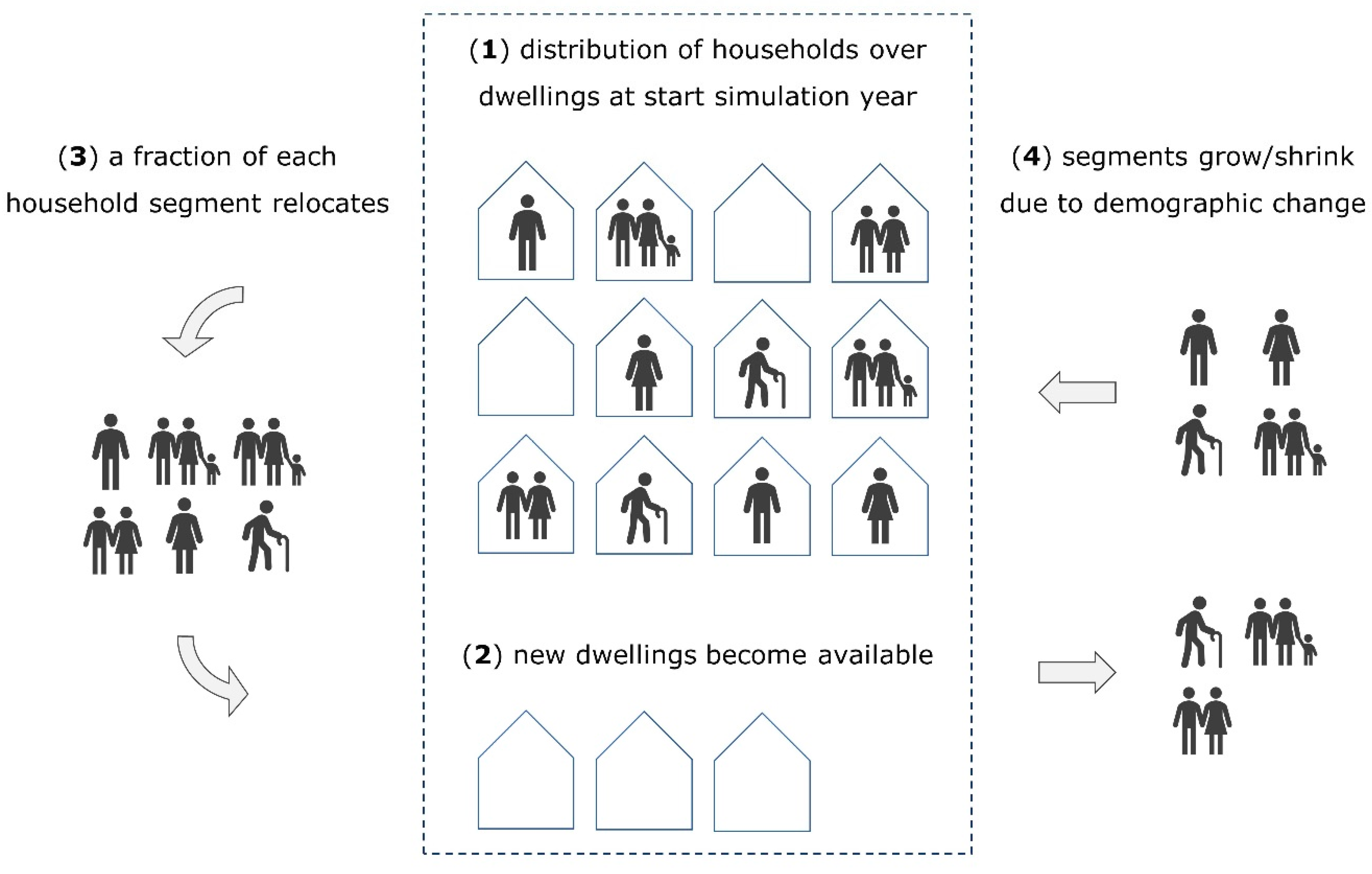
The microsimulation starts with a given distribution of households at the ward level, belonging to one of the 12 segments, over all of the dwellings in the study area (Figure 3). Households are considered the agents of choice, relocating as a single unit between dwellings. Dwellings are the choice alternatives and are spatially defined on a statistical ward level. Each ward is characterized by a set of location features and a residential capacity, i.e., the number of dwellings, which is updated yearly. For simplicity, we assumed that each dwelling can host one household of any segment. Due to the lack of more spatially detailed data, we also assumed that all dwellings that belong to the same ward have identical attributes, being the characteristics of the ward in which they are located. Simulation was performed in yearly time steps, the distribution of households at the start of each year depending on the output of the previous simulation year. During each simulation year, residential dynamics were emulated by means of relocation and demographic change. Demographic change is evaluated last, after relocations have occurred, to ensure that yearly simulation output respects the HPROM projections defined on a district level.

4.2.6. Allocation

The allocation module takes lists of relocating or newly formed households, respectively provided by the relocation and demographic change modules, and allocates them to individual dwellings. Allocations are performed iteratively and in a random order. The dwelling that a relocating household is leaving is first randomly sampled. For this sampling, we use the distribution of the corresponding segment at the start of the simulation year as weights. Then, the relocating household is probabilistically allocated to a new dwelling, using the choice probabilities derived from Equation (2). Dwelling occupancy is updated after each allocation. Occupied dwellings have their choice probabilities set to zero for subsequent allocations. Dwelling utilities are updated at the start of each simulation year.

4.2.7. Relocation

During each simulation year, the number of relocations for each segment is estimated. For this we used relocation fractions derived from the number of observed relocations/non-relocations between the start of 2003 and 2004 (Figure 4). This information was derived from the microsample made available for this research. We multiplied these fractions with the current populations of the corresponding segments to produce a list of all relocations to be performed. This list was then passed on to the allocation module discussed above.

4.2.8. Demographic Change

The demographic change module provides yearly predicted changes in household populations per district. If a segment decreases in size, a corresponding number of households is randomly removed from the district. If a segment increases in size, a corresponding number of entries are added to a list of households to be allocated to a dwelling in the district. As before, this list is then passed on to the allocation module. Demographic change between 2001–2011 was derived from linear interpolation between the observed values of the last two Censuses. For the period 2012–2040, we used the HPROM model from the Federal Planning Bureau [61,68]. HPROM covers the natural growth, migration and household (de)formation components of demographic change. To refine the LIPRO typology [76] used in HPROM to our 12 household segments, we used membership rates of segments versus LIPRO classes. This information was derived from the 2011 Census data.

4.2.9. Accuracy Assessment

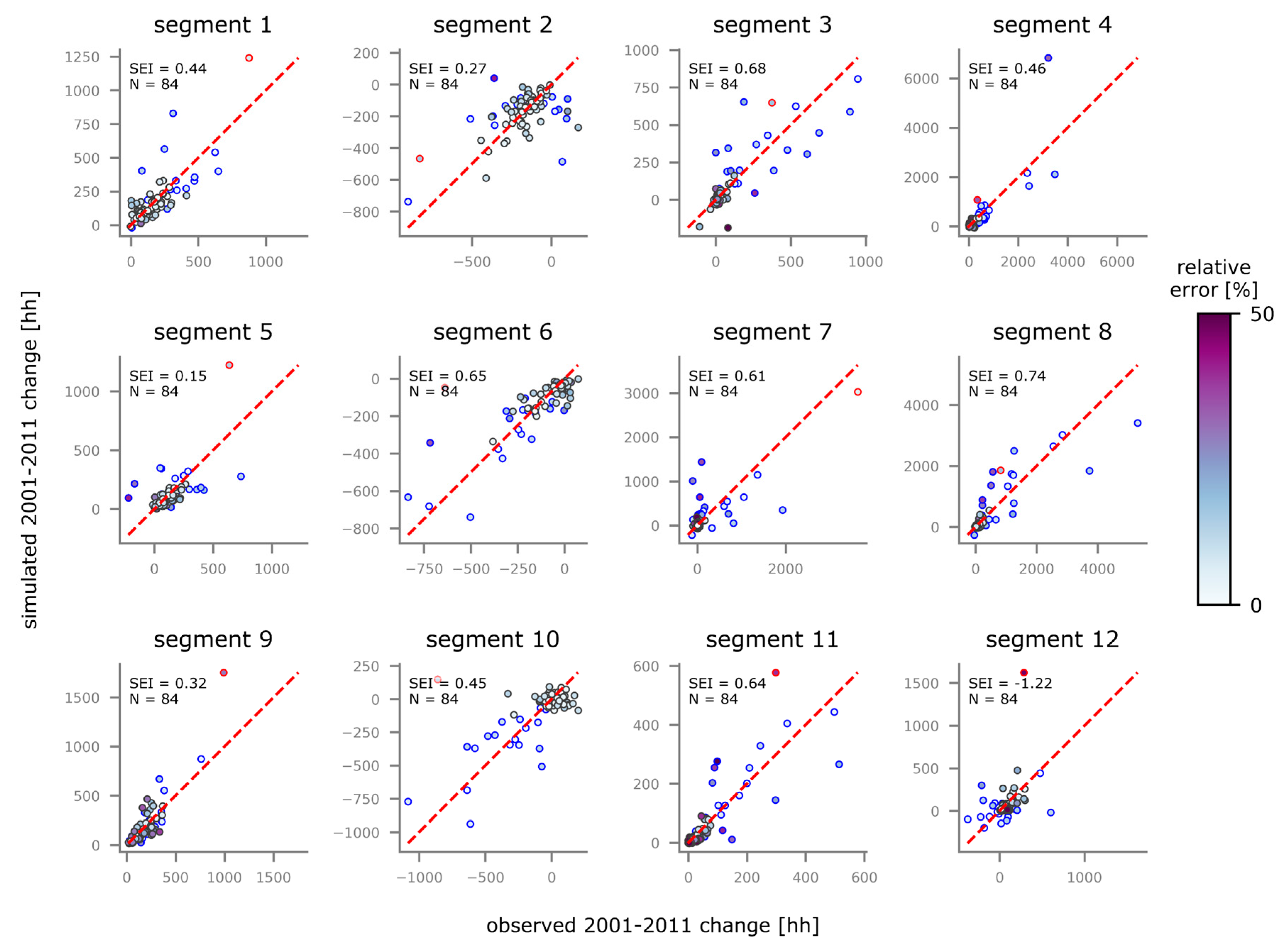
To assess to what extent the RM framework can recreate past residential dynamics, simulation was performed between 2001 and 2011, the years of the last two Censuses. Similar to demographic change for this time period, the yearly number of dwellings per statistical ward was derived by linearly interpolating the number of dwellings between 2001 and 2011. Considering the stochastic component of RM and the high level of spatial detail on which dwellings are defined (wards), some degree of spatial aggregation was required to properly assess simulation performance [77]. Hence, validation was performed on the 84 municipalities in the study area. Also, since the objective of RM is to simulate household location dynamics, we focused on assessing the accuracy of simulated changes per household segment. Scatterplots visualizing simulated versus actual change between 2001 and 2011 were made for each household segment, similar to [38]. To quantify the extent to which the scatterplot point cloud approximates the diagonal line, the latter representing perfect accuracy, a measure called Standard Error around Identity (SEI) was used. SEI is defined here as:
S E I = 1 m = 1 M ( y e s t , m y r e f , m ) 2 m = 1 M ( y r e f , m y ¯ r e f ) 2
with yest change in households estimated by means of simulation, yref observed change in households or a reliable estimate thereof, y ¯ r e f the mean of yref, M the number of municipalities [31]. SEI values range between an arbitrary negative value and a maximum positive value of 1. SEI values of 1 indicate perfect accuracy [77].
When spatiotemporally modelling change of any kind, it is considered good practice to check that the proposed model outperforms a random model [78,79,80]. In this study, a random model is defined as a model with uniform dwelling utilities for each household segment, meaning that each dwelling has an equal probability to be chosen by any household. SEI values of simulated changes obtained with the proposed and uniform utility models were compared, both overall and on a per-segment basis. Overall SEI is defined as a weighted average of per-segment SEI values:
S E I ¯ = s = 1 S h s h j   S E I s
with hs the 2011 total number of households from segment s and S the number of household segments, i.e., 12.

4.3. Scenario Definition

4.3.1. Rationale for Scenario Definition

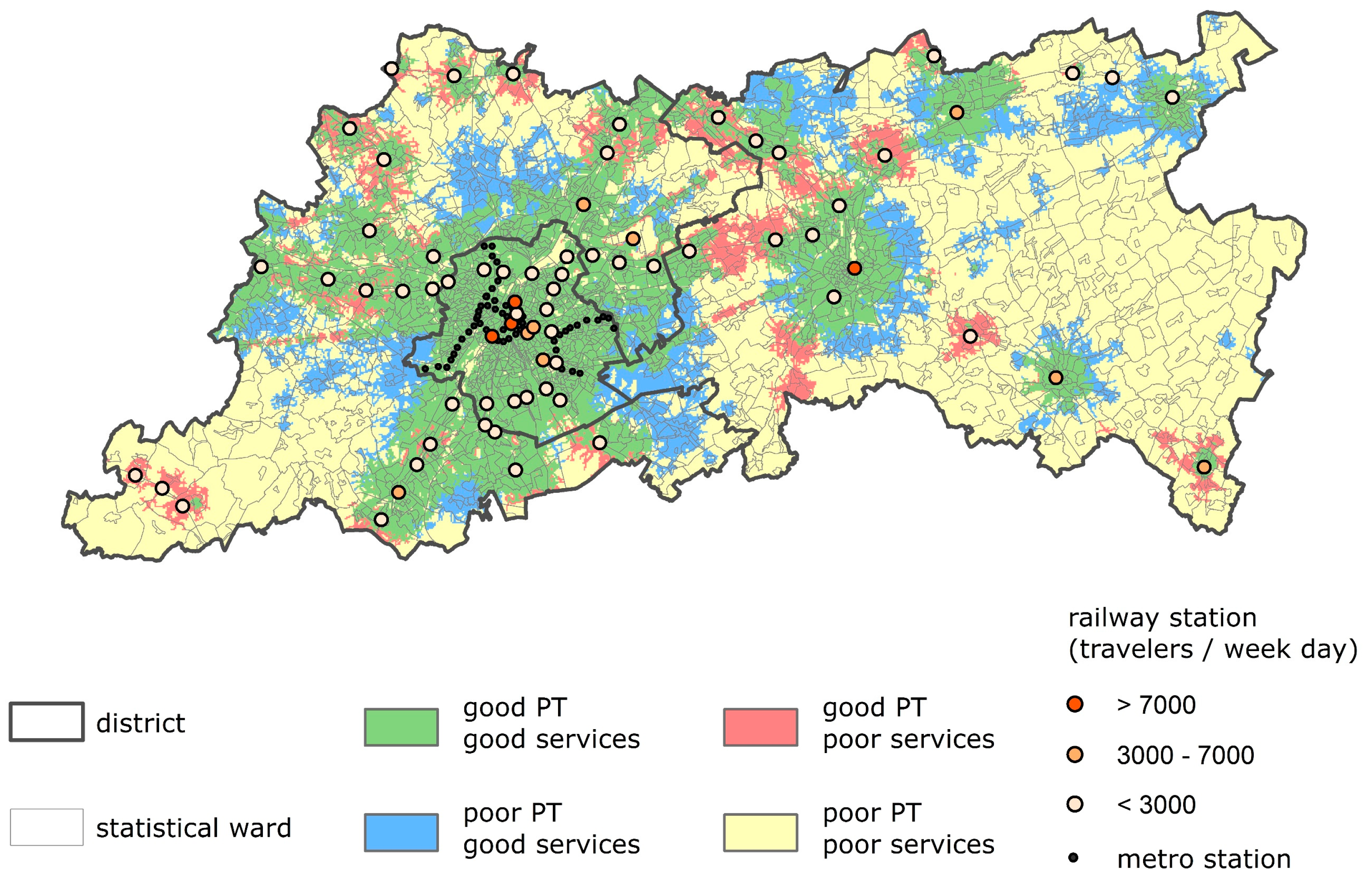
In this study, scenario analysis was used to explore alternative futures in terms of how spatial planning policy affects residential dynamics in the study area. The baseline scenario BAU assumed a continuation of current planning practices. In this scenario, new residential development can occur in any area where zoning allows it, without spatial prioritization. An alternative scenario, SUS, envisioning a more sustainable form of urban planning, was also defined. The SUS scenario draws on the spatial planning strategies of the Flemish and Brussels regional governments. The main objective of the Spatial Policy Plan for Flanders (SPPF) is to achieve a more sustainable form of spatial planning that addresses expected demographic and socioeconomic changes in Flanders over the coming decades. It envisions the concentration of new development near already built-up areas, with the intent of achieving a higher spatial efficiency, protecting remaining open spaces, countering urban sprawl and decreasing private car usage. The densification of the existing urban fabric is an important tool to achieve these goals [14]. The Brussels Regional Plan for Sustainable Development (RPSD) defines 12 high-priority neighbourhoods to address its future expansion. These neighbourhoods are intended to spatially connect high-density residential–economic activity with the blue and green network, and with the transport networks of the region. Decreasing private car use is one of the core objectives of this strategy [15]. In addition to the RPSD, the Brussels region has also developed an urban renewal plan dedicated to its canal area [81]. Both the SPPF and RPSD acknowledge the importance of interregional cooperation, particularly in addressing the dire mobility situation plaguing the BCR and its Flemish vicinity. Considering the importance of more sustainable mobility for both regional spatial strategies, it makes sense that the SUS scenario uses (metro) railway station neighbourhoods as priority areas for denser urban development. Figure 5 shows that the vicinities of railway stations are generally characterized by good access to public transport and services [62].

4.3.2. Implementing the Two Scenarios

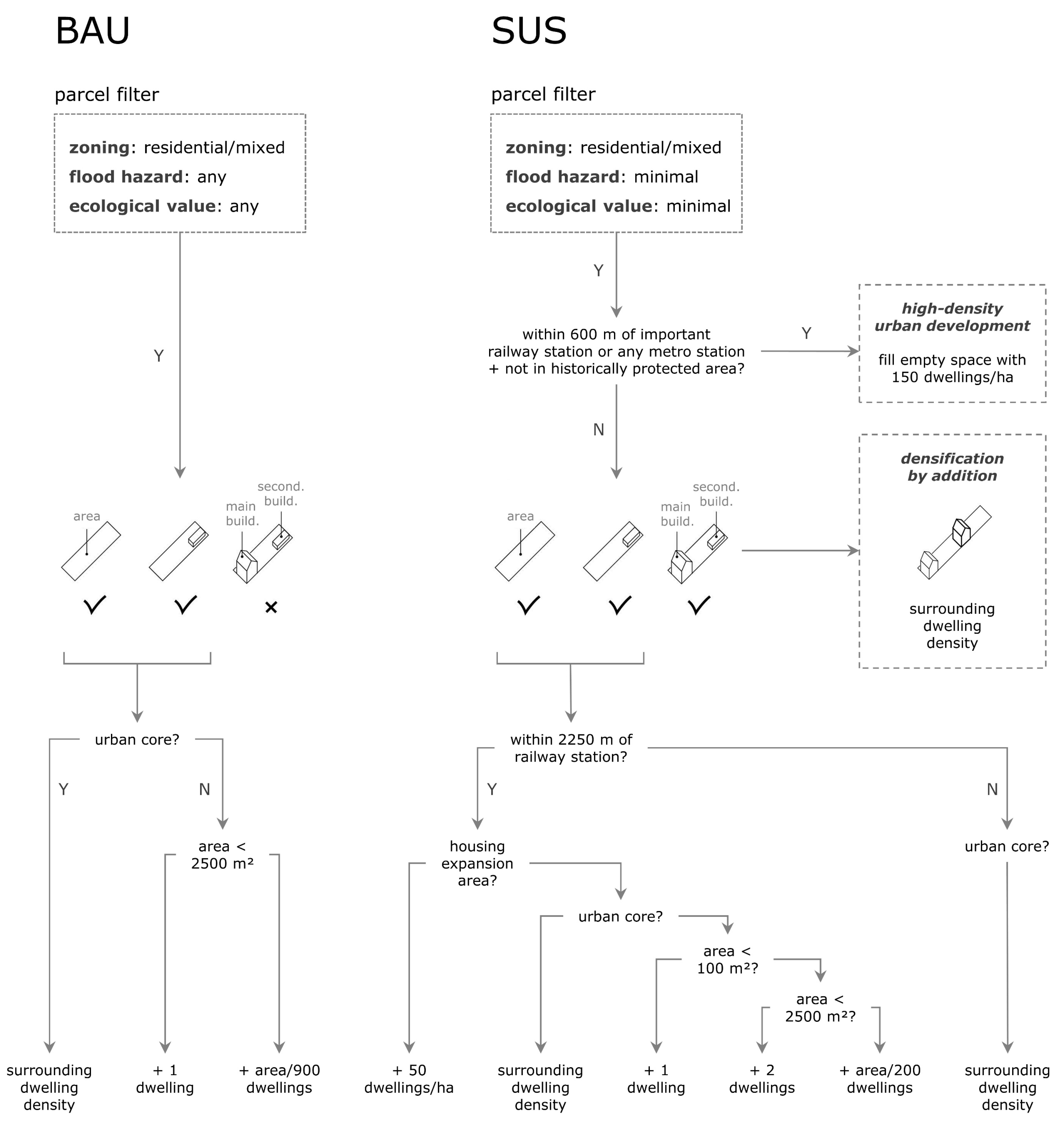
A set of residential constraints, i.e., yearly estimates of dwellings per ward, were defined for each scenario. The constraints guided microsimulation beyond 2011, which was considered to be the current situation given the data used. Decision trees were designed for each scenario to estimate the maximum number of extra dwellings per statistical ward, on top of the dwellings already present in 2011 (Figure 6). The decision tree analysis was performed on a parcel level using land registry and other data, though results were used on ward level.
BAU decision tree requires parcels eligible for new development to be unbuilt and located in residential zoning or mixed zoning, including residential. BAU does not consider access to public transport, services, flood risk or ecological value. Each new parcel outside an urban core that is less than 2500 m2 in size can only contain one dwelling. This area threshold was based on a random sample of parcels containing at least one building. Larger parcels are divided in units of 900 m2 per household, which is the Flemish average. In the BAU scenario, only parcels located in urban cores are considered for denser dwelling development, following the surrounding dwelling density. Here we defined urban cores morphologically based on ward-level surface sealing being at least 25%.
In the SUS scenario, residential development is firstly limited to low flood hazard and to areas with low ecological value. Contrary to BAU, both built-up and free parcels are considered for new development. Empty parcels within 2250 m of railway stations are candidates for denser development. The 2250 m threshold represents a short trip covered by bike or public transport [82]. The highest dwelling densities are appointed to housing expansion areas, i.e., currently empty reserve areas for new residential development, within the above-mentioned distance from train stations. Note that contrary to BAU, SUS uses a default residential parcel size of 200 m² instead of 900 m². Empty parcels located further than 2250 m from railway stations are only developed in this scenario if they are located in an urban core. Built-up parcels follow a separate branch in the decision tree and are densified using surrounding dwelling density. Another separate branch of SUS decision tree is dedicated to parcels located within 600 m of important railway stations or any metro station, regardless of whether they are built-up or not. A railway station is considered important if at least 2000 travellers use it on an average weekday. The 600 m distance threshold represents short trips on foot [82]. Here, empty space within non-historically protected parcels is densified up to 150 dwellings/ha. Overall, residential development is denser in SUS.
Starting with the 2011 housing stock, it was assumed that, in the simulation, housing supply on a district level follows demand dictated by the total number of households plus a 5% margin where possible. Ward level housing stock never exceeds the scenario-based constraints. In BAU iterative random sampling of new dwelling locations is applied over all wards until the current year’s housing demand is met. SUS uses sampling weights proportional to the maximum number of extra dwellings per ward, reflecting the prioritization of new residential development in areas that are deemed more interesting according to the logic of the scenario.
Two microsimulations were performed using the residential constraints of the BAU and SUS scenarios. Apart from the yearly estimates of dwellings per ward, all simulation input was the same. Simulations begin in 2011, using observed household distributions from the last Census, and progress to 2040. The output of the two simulations was mapped, analysed and compared.

5. Results

5.1. Microsimulation Performance

Microsimulation was performed between 2001 and 2011 using choice probabilities derived from the household location choice models fitted for each household segment. The summaries of these conditional logistic regression models are shown in Appendix A of this document (Table A1). Validation scatterplots showing simulated versus observed changes in numbers of households per segment are shown in Figure 7. Visual inspection of the scatterplots indicates that the microsimulation correctly reproduces positive and negative trends for each segment. Most observations, i.e., municipalities, are situated close to the 1:1 line of the scatterplots. Most relative errors, i.e., the absolute error divided by the 2011 number of households per corresponding segment, are reasonably small, ranging between 0% and 20%. Some larger errors can, however, be observed. An examination reveals that for 9 out of 12 segments, the municipality of Leuven exhibits the largest absolute error (dots with red edges in Figure 1). The municipalities of the BCR (dots with blue edges in Figure 1) also often display large errors. Except from segment 12 (renting households whose reference person is older than 60 and does not hold a higher education degree), all household segments have SEI values larger than 0.
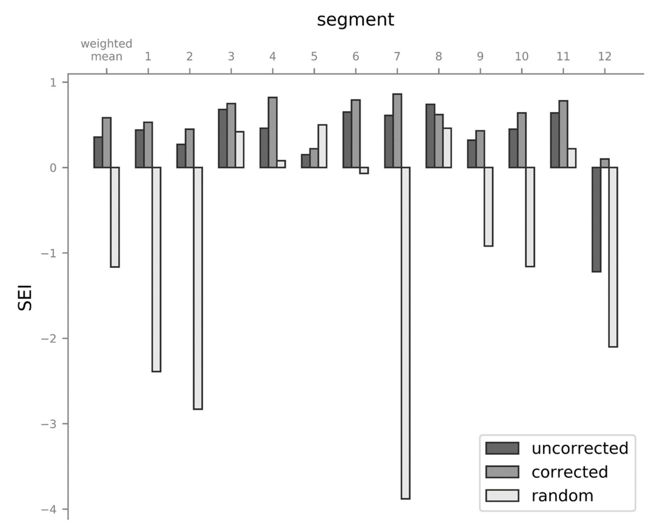
To perform a somewhat fairer assessment of the microsimulation’s performance, outlier errors were removed from the scatterplot and SEI values were recalculated (Figure 8). Outlier errors were identified here as errors located further than 3 standard deviations from the mean error. Between 1 and 3 outliers were identified and removed per segment. In addition, a comparison was made with simulation accuracy obtained with a uniform household location choice model, i.e., one with identical utilities for each dwelling. Note that all segments have positive SEI values for the corrected output, and 8 out of 12 segments have SEI values over 0.5. Segment 12 still has a notably low simulation accuracy after correction, with SEI equal to 0.1, though its improvement compared to the uncorrected SEI is the largest of all segments. Apart from segment 5 (homeowner households without children and a reference person younger than 60 holding a higher education degree), all household segments have higher SEI values for the proposed simulation compared to simulation with a random model. The weighted average SEI values are 0.35 and 0.58 for the uncorrected and corrected simulation output respectively. For the random model, overall SEI amounts to −1.16.

5.2. Scenario Predictions

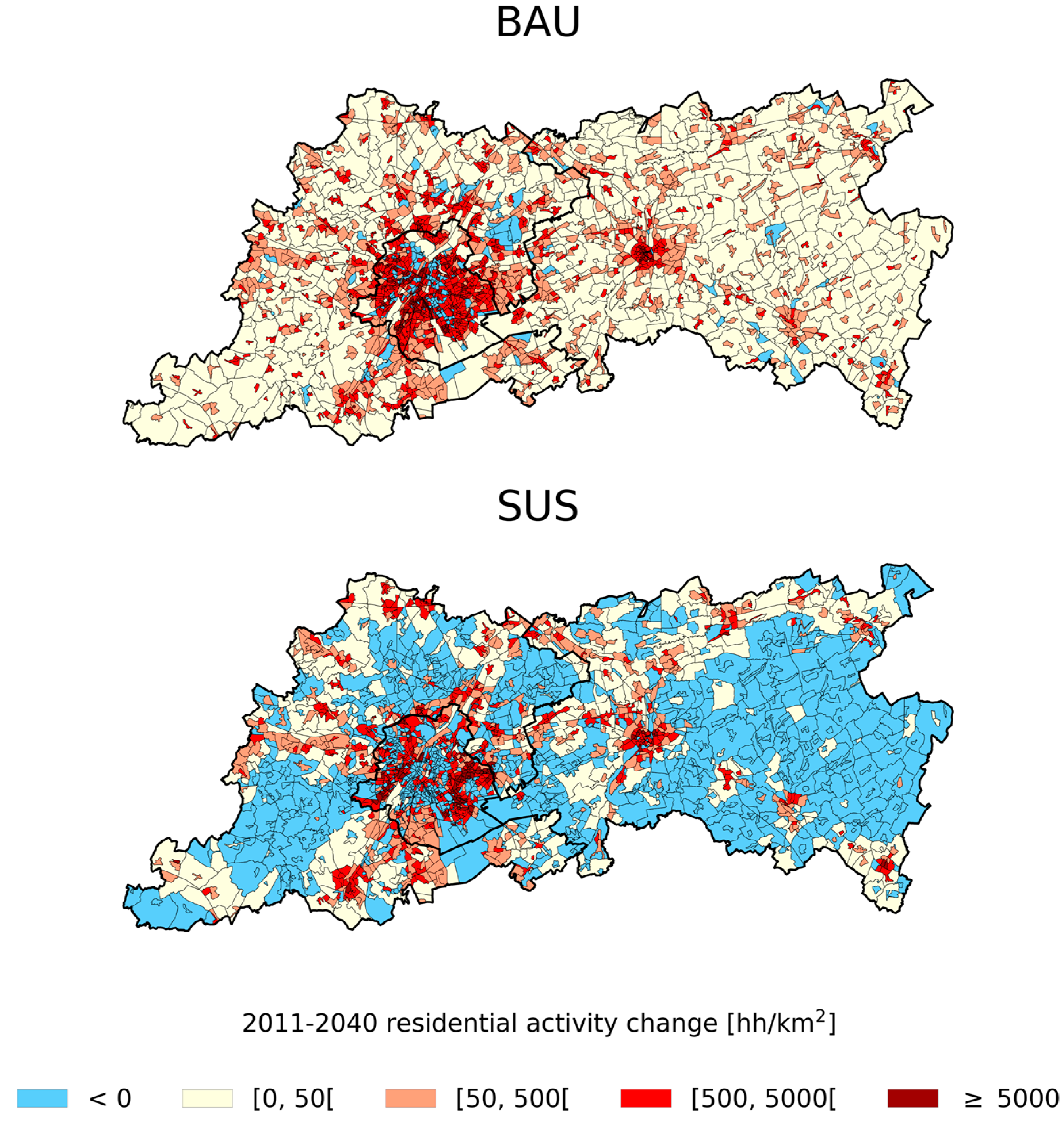
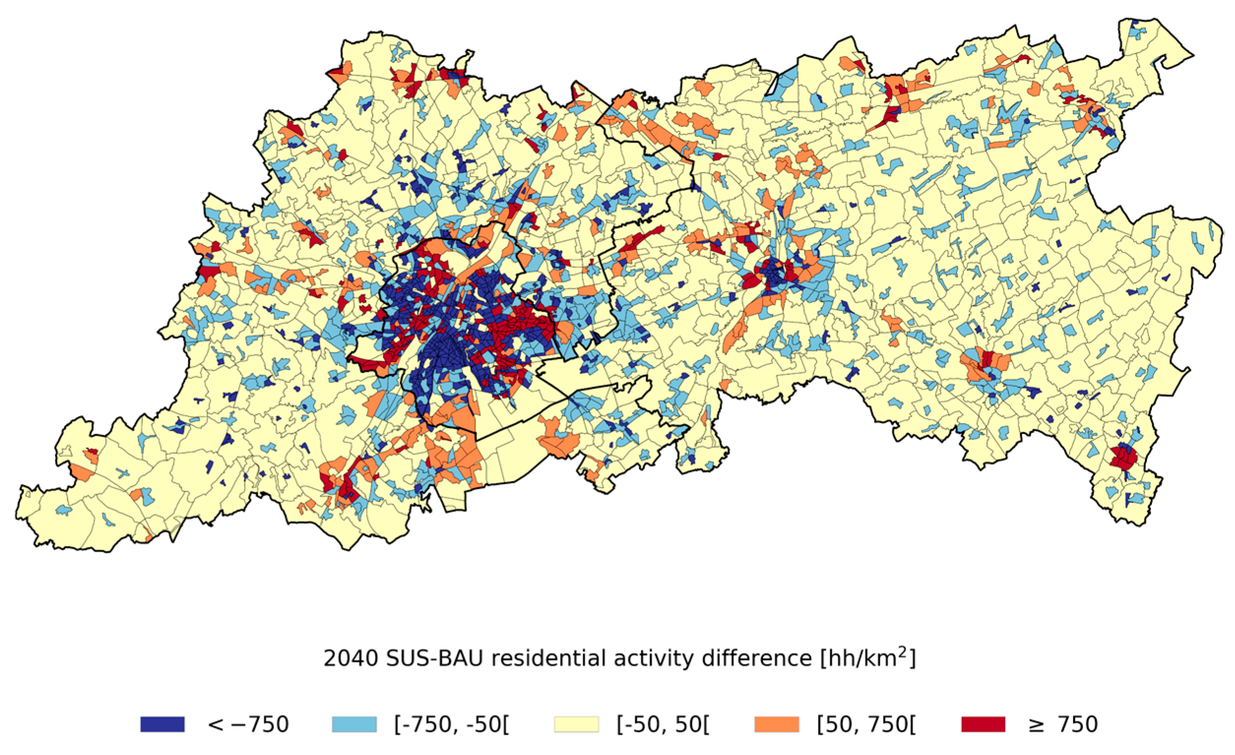
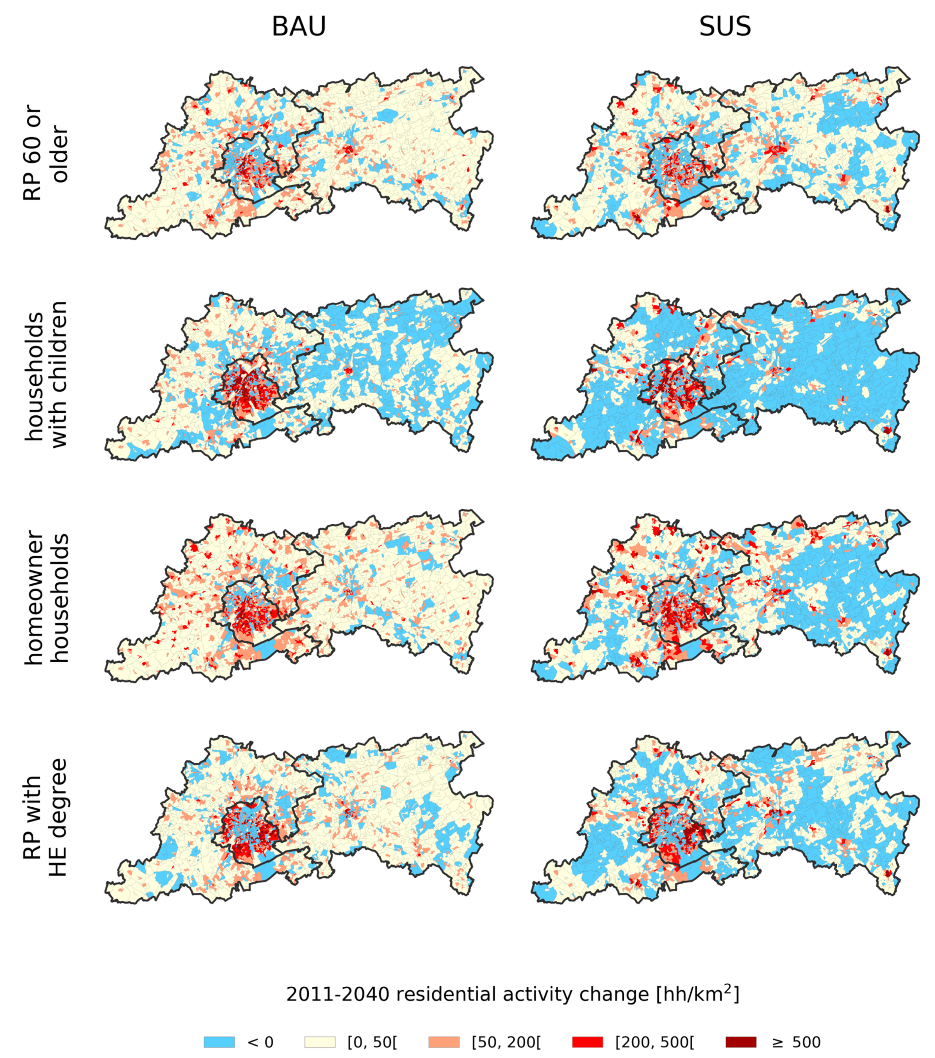
Microsimulation was performed between 2011 and 2040 using the HPROM derived demographic projections and the BAU and SUS scenario constraints. Overall district-level changes in residential activity are equal for each scenario; only their spatial distribution over wards differs. Figure 9 shows the simulated changes between 2011 and 2040. Figure 10 shows the differences between the 2040 scenarios. The inspection of both maps reveals that new development in SUS is spatially more concentrated compared to simulated development in BAU. Remote, poorly serviced rural areas are characterized by negative change in SUS, whereas the same areas often have strong growth in BAU. Within the BCR, SUS development is grouped around public transport hubs whereas BAU development is spread out over the region, with some degree of clustering in the municipalities of Sint-Gillis and Vorst, south of the city center of Brussels.
Outside the BCR, SUS development is clustered around secondary (Leuven) and tertiary urban cores, and to a lesser extent in the areas between those cores. BAU development outside the BCR shows some clustering around urban cores, although clearly much of its new residential activity is scattered over the rural areas of the study area.
BAU and SUS simulation results are mapped for different segment groupings in Figure 11. Overall, SUS seems to yield more extreme differences between areas of growth and decline. For households with children, SUS predicts a pronounced concentration of growth near well-serviced urban hubs, resulting in negative growth in most other areas, particularly in the districts of Leuven and Halle-Vilvoorde. Growth of households with a reference person older than 60 seems to be most spread out over the whole study area, both for BAU and SUS. Growth in homeowner households and household with a RP holding a higher education degree is quite dispersed within the districts of Leuven and Halle-Vilvoorde, yet in SUS these households are drawn to the higher-density development areas identified by the scenario.

6. Discussion

6.1. Considerations Regarding Microsimulation Performance

The validation of the RM performed between 2001 and 2011 shows its capability to reproduce changes in residential activity with reasonably accuracy. We show that the proposed models clearly outperform a uniform household location choice model assigning households randomly to available dwellings. Some issues remain to be addressed. From a methodological point of view, we acknowledge that microsimulation performance may be improved by using more advanced discrete choice algorithms, such as nested and mixed logistic regression [64,72,83]. These techniques are better suited to address issues such as agent heterogeneity and spatial autocorrelation. Such models are, however, also more difficult to calibrate, and do not always yield expected increases in modelling accuracy [84].
The inspection of simulation performance shows that the municipality of Leuven exhibits disproportionally large errors for each household segment. This can be explained by the fact that Leuven is a university city with a high share of residing students relative to its population. Belgian fiscal policy makes it advantageous for students to formally reside with their parents while renting a second student home in the city where they study. As a result, considerable portions of the housing stock in university cities are taken up by people that are not official residents. The issue of dealing with student populations in RM for the UK is addressed in [33,85]. Yet, for this study it was not possible to obtain reliable data to account for this phenomenon. Secondly, we observe that the microsimulation performs poorly, in terms of 2001–2011 accuracy, for segment 12, i.e., older lower educated renting households. This is somewhat to be expected, given that the more complex housing situations of this segment (retirement/nursing homes, service flats, intergenerational living, social housing reserved for elderly) are difficult to capture with the limited data at our disposal.

6.2. Scenario Analysis

This paper focuses on the definition of a spatial simulation framework for policy-inspired scenario assessment. Such an exercise is necessarily bound to the political and socio-economic realities of the area on which it is performed. The results obtained with the household location choice models (Figure 7 and Figure 8) and the scenario-based microsimulation (Figure 9, Figure 10 and Figure 11) should thus be interpreted in light of the rather unique context of residential dynamics in Flanders. Many Flemings prefer to live close to their family network [86] and/or live in a suburban–rural neighbourhood [87]. This behaviour effectively reduces the number of longer distance relocations and contributes to the societal normalization of commuting. Suburban–rural living, and the private car commuting needed to support it, are made fiscally attractive in Belgium, e.g., by heavily subsidizing company cars [88]. Many Flemings perform long distance commutes to Brussels on a daily basis. In addition to congestion and its many related issues, this contributes to the absence of a clear spatial pattern in the residential locations of the Brussels workforce, contrary to most other European cities [89].
The urban planning scenarios developed for this research represent alternative forms of spatial planning policy, with BAU akin to weak regulation and SUS representing strong regulation in favour of residential development in well-serviced areas. Some of the simulated differences between the 2040 scenarios may have a considerable impact on municipal socioeconomic fabric and fiscality. Compared to BAU, SUS scenario predicts much more concentrated growth of households with children, homeowner households and higher educated households around urban cores, whereas older households are spread out more evenly over the study area. SUS even predicts net 2011–2040 negative growth in households for most rural areas of the study area. Whereas this may make sense from a sustainable transport perspective, it is likely that measures leading to this outcome will face resistance from rural populations, unless suitable financial compensation is provided for planned changes in land use. It is also likely that policies promoting relocation to more urbanized areas will face resistance from many Flemings who generally prefer rural/suburban living [86,87]. The increase in residential activities in urban areas predicted by SUS are founded on a spatially explicit analysis of available space on a parcel level, using areal estimates based on insight from contemporary urban planning. Yet, these higher densities will have far-reaching implications on how urban spaces are to be designed, including the private, public or ecosystem facilities needed to support such densities. Policy-makers, planners and other stakeholders must consider how further increasing density in an area that is already quite densely urbanized, the BCR, will impact living conditions, and if they are prepared—both politically and logistically—to take the measures required, and to maintain them over longer periods of time, in order to guide this process to an outcome that ultimately benefits a large majority of the population. We believe, however, that the highest dwelling density proposed in this research (150 dwellings/ha) allows sufficient provision of green space, services and other urban qualities, if designed properly.
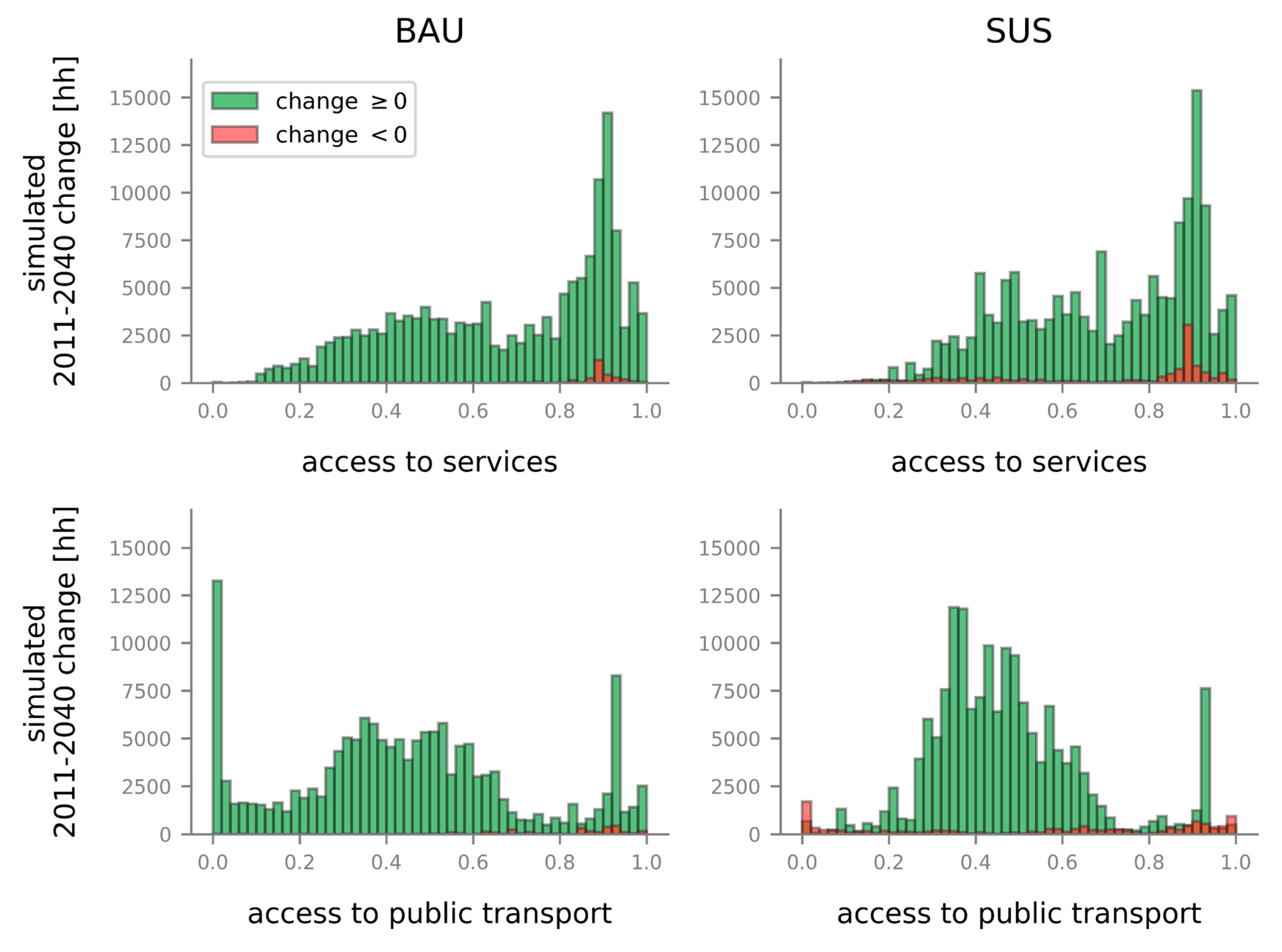
Obviously, the performed scenario analysis has its shortcomings, one of them being that it only covers two visions of future urban development — for the rather complex case-study of BCR–Flanders. Secondly, we only explored the impact of differing spatiotemporal distributions of housing stock defined according to the logic of our urban development scenarios. It goes without saying that many more factors play important roles in the process of future urban development, including social inequality, transport infrastructure, social housing, financial crises, urban economy, real estate, and the popularity of alternative housing strategies (e.g., co-housing). However, as stated above, the proposed scenario-driven RM is not intended to be final or exhaustive, but only to show that it can be of use to explore the impact of alternative planning decisions, and how this can contribute to a better informed debate on the recently proposed strategies of Flanders and the BCR. One possible way to do this would be by quantifying where 2011–2040 demographic growth will be located in terms of current access to public transport and services, as determined by [62]. Such a possible analysis is illustrated in Figure 12, which shows histograms weighed according to predicted changes in households on a statistical ward level for each scenario. Both in terms of services and transport, and particularly the latter, the SUS scenario predicts a considerably better 2040 situation compared to residential development predicted by the BAU scenario. Remarkably, while still being considerably better compared to BAU, most SUS growth is located in average public transport accessibility areas. This can be explained in part by the limited space left for new development in areas with good public transport servicing. Another explanation lies in the constraint of the SUS scenario excluding densification in historically valuable neighbourhoods, many of which are located in well-serviced areas of the BCR. This constraint could be partially relaxed in an alternative scenario definition, if deemed necessary. Findings from this, or similar considerations, could in turn be used to quantify related positive impacts, e.g., reductions in transport related greenhouse gas emissions, air pollution or road congestion.
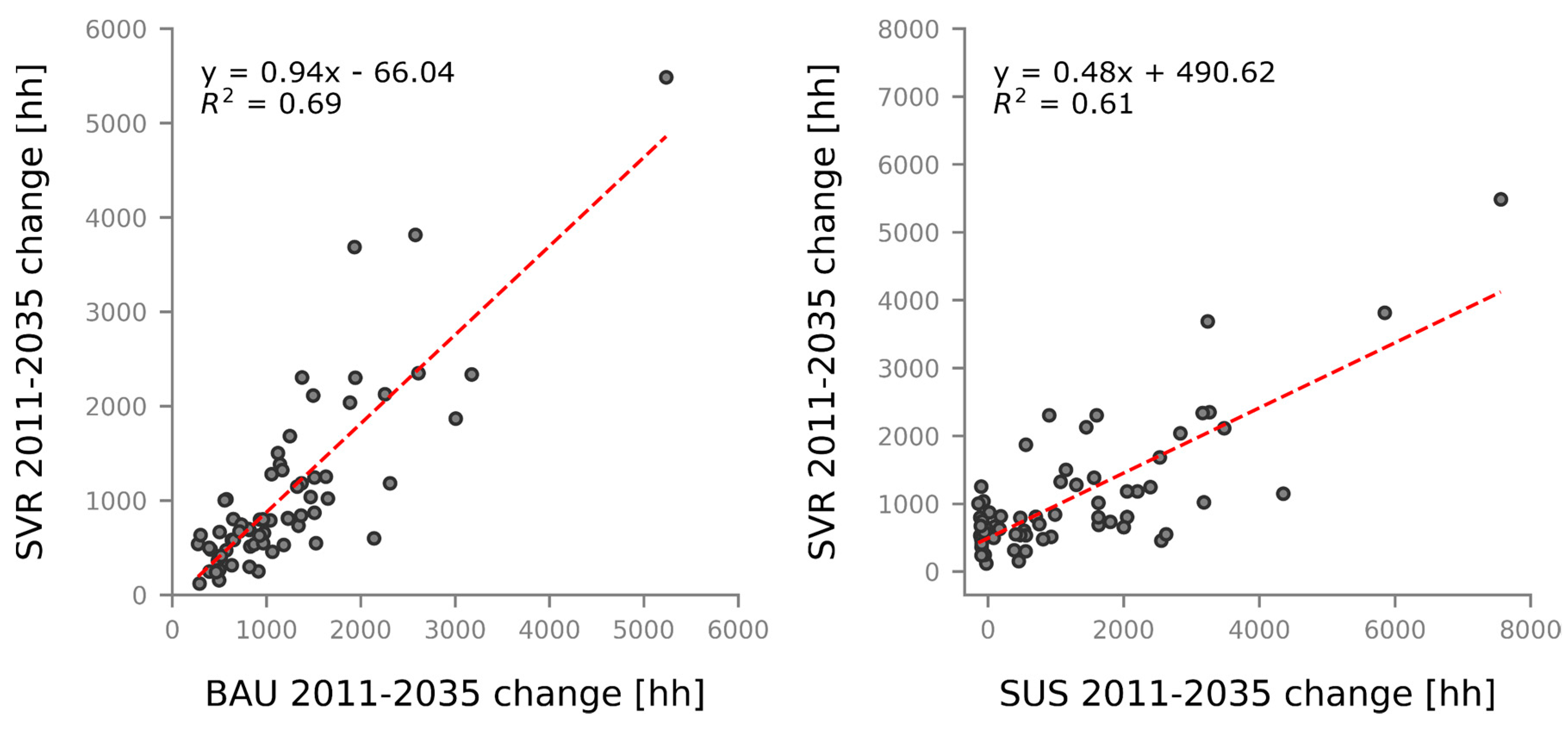
Another potentially interesting way to valorise our microsimulation output would be by comparing it to other demographic projections on spatially detailed geographic units. Such projections have been made at the level of Flemish municipalities up to 2035, named after the Study Department of the Flemish Government (SVR) [90,91]. In Figure 13, a comparison is made between SVR and our own 2011–2035 projected increases in households over the Flemish municipalities of our study area. Remarkably, BAU predictions seem to correspond strongly to the SVR projections. A comparison to SUS estimates reveals that the SVR projections have more small growth municipalities in which SUS growth is (near) zero or even negative. Conversely, SUS also predicts more concentrated growth compared to the SVR. The SVR projections are based on the cohort-component method [92], which is a stepwise numerical extrapolation approach supported by assumptions of fertility, mortality and migration. The cohort-component method does not take into account spatially explicit information related to how and where expected growth can be allocated. Considering our findings in Figure 13, it could be stated that BAU is in fact similar to a non-spatial scenario, or at least a spatially trivial scenario, representing a mere extrapolation from the 2011 spatial distribution of households, itself a result of decades of urban sprawl. The SUS scenario on the other hand does constitute a clear break with urban sprawl.

6.3. Future Opportunities

This study aims to support the claim that the combined use of RM and scenario analysis should play a more prominent role in integrated urban modelling applications and spatial policy assessment, as recently proposed by [32]. What sets this study apart from earlier research, e.g., [52,53,54,55], is its focus on providing a more formal scenario analysis that draws on an extensive set of revelant spatial data. In addition, we explain in detail which urban planning logic and assumptions are used to define our scenarios, as well as how this relates to current and potential future planning practice. As agreed upon in the literature, scenarios should be defined in a transparant reproducable fashion, aiming to be as relevant as possible to the involved stakeholders [42,43,45,46].
Particularly for the selected case study, there is a need for more scientifically grounded information to support, or debunk, different narratives on how we can tackle the issues of urban sprawl and congestion. What is key in this debate, or any discussion involving the future, is open and transparent communication of the assumptions made to support one’s vision. The analysis proposed in this research leaves plenty of room for further refinement. Generally, this research would greatly benefit from a more interdisciplinary approach and the direct involvement of stakeholders, including planning officials, politicians and citizens. Scenario-wise, there are important developments that could be explored by means of microsimulation. One such example is the planned construction of the new North–South metro line in the BCR. Scenario-based RM can be used to assess how this new infrastructure may impact residential patterns in the region, giving a new perspective on this highly debated project. A similar analysis can be performed on the GEN railroad network, an ongoing, yet strongly delayed, project intended to provide better public transport connection between the BCR and its periphery.

7. Conclusions

In this paper a spatial dynamic microsimulation framework is proposed to simulate residential dynamics in the Brussels Capital Region and Flemish Brabant up to 2040. Simulation is based on two scenarios entailing alternative visions on future urban development. The BAU scenario constitutes a status quo with regards to historic urban sprawl, whereas the SUS scenario defines a viable pathway to more compact urban development. Both scenarios are supported by spatially explicit analysis and rely on a set of urban development rules. For SUS, inspiration is further drawn from recently formulated strategic policies in Flanders and the Brussels Capital Region.
The validation over the time period between the last two national Censuses shows that the proposed simulation approach succeeds in modelling past trends, at least on a municipality level, outperforming a random model. Running the BAU and SUS scenarios until 2040 results in different evolutions of ward-level housing stocks. The scenario-based microsimulation results suggest potentially far-reaching implications: BAU leads to even more urban sprawl; SUS counters this trend at the cost of strong concentration of growth around urban cores, particularly for the younger household segments. Spatially detailed information on future distributions of different types of households as provided by the scenarios may be of use to assess the economic, social and environmental impacts of alternative pathways of urban development to make better informed decisions on a spatial policy level and to better prepare for their outcomes. With this work, we contribute to an emerging body of research underlining the value of spatial microsimulation, used in combination with scenarios, for policy assessment or integrated urban modelling [32,34,51]. We believe that the modelling approach proposed in this study, and the outcomes of the scenario analysis presented, will positively contribute to the ongoing debate on countering urban sprawl in Flanders.

Author Contributions

F.P. and F.C. designed the research strategy. F.P. implemented and performed the experiments, analyzed the results and wrote the draft for the manuscript. P.S. designed the decision trees supporting the scenario analysis and provided expertise on planning praxis in Brussels-Flanders and contemporary sustainable urban planning. F.P., P.S. and F.C. reviewed and edited the manuscript. All authors have read and agreed to the published version of the manuscript.

Funding

The research pertaining to these results received financial aid from the Federal Science Policy (BELSPO) per the agreement of subsidy no SR/00/307 (UrbanEARS), SR/67/167 (BELAIR 2013), SR/XX/170 (BELAIR SONIA) and SR/03/333 (BELAIR SONIA 2015).

Acknowledgments

We acknowledge the datasets provided by all institutes listed in Table 1. Particular gratitude goes out to Statistics Belgium for their support in providing Census data in requested formats.

Conflicts of Interest

The authors declare no conflict of interest.

Appendix A

Table A1. Summaries of the conditional logistic regression models fitted for each household segment. See Table 2 for household segment definitions.
Segment 1
N = 1000
McFadden R² = 0.073
AIC = 4284
LL = −2135
Featurecoefstd errzP>|z|[0.0250.975]
Household density−0.07660.052−1.4860.137−0.1780.024
Job density−0.08740.065−1.3450.179−0.2150.04
% attached single dwelling houses or apartments0.15610.0821.9070.057−0.0040.316
% social housing−0.09820.044−2.2160.027−0.185−0.011
% households with children0.21020.072.9980.0030.0730.348
% households owning their dwelling0.47250.0945.01200.2880.657
% households with RP having a HE degree0.38280.03710.46700.3110.455
Segment 2
N = 1000
McFadden R² = 0.086
AIC = 4217
LL = −2103
Featurecoefstd errzP>|z|[0.0250.975]
Distance to nearest highway entrance/exit0.0740.0352.1070.0350.0050.143
% households with RP younger than 600.32870.0843.90700.1640.494
% households with children0.18950.0762.4970.0130.0410.338
% households owning their dwelling0.46560.0637.40300.3420.589
% households with RP having a HE degree−0.4720.049−9.6240−0.568−0.376
Segment 3
N = 1000
McFadden R² = 0.07
AIC = 4297
LL = −2141
Featurecoefstd errzP>|z|[0.0250.975]
Employment potential−0.08180.052−1.5740.115−0.1840.02
Job density−0.09250.051−1.8220.068−0.1920.007
% attached single dwelling houses or apartments0.40490.0834.87200.2420.568
% households with RP younger than 60−0.39520.069−5.7620−0.53−0.261
% households with children0.57830.0797.32300.4240.733
% households owning their dwelling−0.53080.073−7.2260−0.675−0.387
% households with RP having a HE degree0.60940.03915.58100.5330.686
Segment 4
N = 1000
McFadden R² = 0.104
AIC = 4137
LL = −2063
Featurecoefstd errzP>|z|[0.0250.975]
Household density−0.09260.038−2.4690.014−0.166−0.019
% attached single dwelling houses or apartments0.4520.0815.60600.2940.61
% households with children0.67750.0719.53400.5380.817
% households owning their dwelling−0.67220.064−10.4430−0.798−0.546
% households with RP having a HE degree−0.16440.047−3.5310−0.256−0.073
Segment 5
N = 1000
McFadden R² = 0.039
AIC = 4437
LL = −2302
Featurecoefstd errzP>|z|[0.0250.975]
Job density−0.0670.046−1.4420.149−0.1580.024
% attached single dwelling houses or apartments0.31490.0734.34200.1730.457
% households with RP younger than 600.25810.0753.4190.0010.110.406
% households with children−0.28730.078−3.6970−0.44−0.135
% households owning their dwelling0.71750.0927.79800.5370.898
% households with RP having a HE degree0.31210.0398.08600.2360.388
Segment 6
N = 1000
McFadden R² = 0.057
AIC = 4355
LL = −2170
Featurecoefstd errzP>|z|[0.0250.975]
Access to services0.10920.0591.8490.064−0.0070.225
Employment potential−0.13720.058−2.3810.017−0.25−0.024
Job density−0.11060.069−1.6050.108−0.2460.024
% households with RP younger than 600.53040.0856.21400.3630.698
% households with children−0.44870.077−5.8530−0.599−0.298
% households owning their dwelling0.73010.0947.75800.5460.915
% households with RP having a HE degree−0.33720.047−7.1480−0.43−0.245
Segment 7
N = 1000
McFadden R² = 0.156
AIC = 3903
LL = −1942
Featurecoefstd errzP>|z|[0.0250.975]
Distance to nearest highway entrance/exit−0.12140.065−1.8590.063−0.2490.007
Household density0.0630.0441.4230.155−0.0240.15
Employment potential−0.12210.058−2.1010.036−0.236−0.008
% attached single dwelling houses or apartments0.37540.1043.6200.1720.579
Average house selling price0.10930.0452.4230.0150.0210.198
% households with RP younger than 600.44540.0765.86100.2960.594
% households with children−0.20640.087−2.3840.017−0.376−0.037
% households owning their dwelling−0.19770.094−2.0970.036−0.383−0.013
% households with RP having a HE degree0.39010.0626.25500.2680.512
Segment 8
N = 1000
McFadden R² = 0.094
AIC = 4191
LL = −2086
Featurecoefstd errzP>|z|[0.0250.975]
Access to services0.15720.1011.550.121−0.0420.356
Household density−0.07070.043−1.6350.102−0.1550.014
Employment potential0.14280.0622.3010.0210.0210.264
Job density−0.10360.04−2.5770.01−0.182−0.025
% attached single dwelling houses or apartments0.2630.1192.2160.0270.030.496
% households with RP younger than 600.30420.0734.15200.1610.448
% households with children−0.34080.09−3.7880−0.517−0.164
% households owning their dwelling−0.23910.076−3.1290.002−0.389−0.089
% households with RP having a HE degree−0.30490.054−5.6950−0.41−0.2
Segment 9
N = 1000
McFadden R² = 0.153
AIC = 3912
LL = −1949
Featurecoefstd errzP>|z|[0.0250.975]
Distance to nearest highway entrance/exit−0.10190.055−1.860.063−0.2090.005
Access to services−0.16820.084−1.9980.046−0.333−0.003
% attached single dwelling houses or apartments0.39470.0954.14600.2080.581
% households with RP younger than 60−0.81480.078−10.4440−0.968−0.662
% households with children0.25720.0862.9840.0030.0880.426
% households owning their dwelling0.3270.0973.3820.0010.1380.516
% households with RP having a HE degree0.87610.04121.57900.7970.956
Segment 10
N = 1000
McFadden R² = 0.061
AIC = 4336
LL = −2163
Featurecoefstd errzP>|z|[0.0250.975]
Distance to nearest highway entrance/exit0.12090.0393.1310.0020.0450.197
Employment potential−0.18740.055−3.3890.001−0.296−0.079
% attached single dwelling houses or apartments0.30460.0714.31700.1660.443
% households with RP younger than 60−0.36450.067−5.4190−0.496−0.233
% households owning their dwelling0.55330.0866.42700.3850.722
Segment 11
N = 1000
McFadden R² = 0.13
AIC = 4019
LL = −2003
Featurecoefstd errzP>|z|[0.0250.975]
% attached single dwelling houses or apartments0.38520.0735.300.2430.528
% social housing−0.06580.04−1.6530.098−0.1440.012
Average house selling price−0.06250.041−1.5260.127−0.1430.018
% households with RP younger than 60−0.75720.064−11.7890−0.883−0.631
% households owning their dwelling−0.66410.073−9.1480−0.806−0.522
% households with RP having a HE degree0.59940.04912.29500.5040.695
Segment 12
N = 1000
McFadden R² = 0.116
AIC = 4081
LL = −2034
Featurecoefstd errzP>|z|[0.0250.975]
Employment potential−0.07920.051−1.5560.12−0.1790.021
% attached single dwelling houses or apartments0.41040.094.53800.2330.588
% households with RP younger than 60−0.53490.066−8.0730−0.665−0.405
% households with children0.12820.0821.5650.118−0.0320.289
% households owning their dwelling−0.7450.062−11.9370−0.867−0.623
% households with RP having a HE degree−0.09710.05−1.9540.051−0.1940

References

  1. EEA-FOEN. Urban sprawl in Europe; European Environment Agency-Federal Office for the Environment: Luxembourg, 2016; ISBN 9789292137380. [Google Scholar]
  2. De Vos, J. The influence of land use and mobility policy on travel behavior: A comparative case study of flanders and the netherlands. J. Transp. Land Use 2015, 8, 171–190. [Google Scholar] [CrossRef] [Green Version]
  3. Christidis, P.; Ibañez Rivas, N. Measuring road congestion; European Commission-Joint Research Center-Institute for Prospective Technological Studies: Luxembourg, 2012; ISBN 978-92-79-27015-4. [Google Scholar]
  4. Dingil, A.E.; Schweizer, J.; Rupi, F.; Stasiskiene, Z. Transport indicator analysis and comparison of 151 urban areas, based on open source data. Eur. Transp. Res. Rev. 2018, 10. [Google Scholar] [CrossRef]
  5. EEA. Air quality in Europe-2018 report; European Environment Agency: Luxembourg, 2018; ISBN 19778449. [Google Scholar]
  6. Stassen, K.R.; Collier, P.; Torfs, R. Environmental burden of disease due to transportation noise in Flanders (Belgium). Transp. Res. Part D Transp. Environ. 2008, 13, 355–358. [Google Scholar] [CrossRef]
  7. EEA. Annual European Union greenhouse gas inventory 1990–2009 and inventory report 2019; European Environment Agency: Luxembourg, 2019. [Google Scholar]
  8. Stevens, M.; Demolder, H.; Jacobs, S.; Michels, H.; Schneider, A.; Simoens, I.; Spanhove, T.; Van Gossum, P.; Van Reeth, W.; Peymans, I. Flanders Regional Ecosystem Assessment: State and trends of ecosystems and their services in Flanders. Synthesis; Research Institute for Nature and Forest (INBO): Brussels, Belgium, 2015. [Google Scholar]
  9. Pisman, A.; Vanacker, S.; Willems, P.; Engelen, G.; Poelmans, L. Ruimterapport Vlaanderen (RURA). Een ruimtelijke analyse van Vlaanderen; Department of Environment and Spatial Development: Brussel, Belgium, 2018; ISBN 9789040303975. [Google Scholar]
  10. Joachim, M.; Teller, A.; Markus, E.; Grizzetti, B.; Barredo, J.I.; Paracchini, M.L.; Condé, S.; Somma, F.; Orgiazzi, A.; Jones, A.; et al. Mapping and assessment of ecosystems and their services in the EU; Publications office of the European Union: Luxembourg, 2016; ISBN 9789279361616. [Google Scholar]
  11. Baert, L.; Reynaerts, J. Het fileprobleem in Vlaanderen en de impact op bedrijfsprestaties; Research Center for Regional Economics (VIVES): Leuven, Belgium, 2018. [Google Scholar]
  12. De Decker, P. Understanding urban sprawl: the case of Flanders, Belgium. Environ. Plan. A 2011, 43, 1634–1654. [Google Scholar] [CrossRef]
  13. Verhetsel, A.; Van Hecke, E.; Thomas, I.; Beelen, M.; Halleux, J.-M.; Lambotte, J.-M.; Rixhon, G.; Mérenne-Schoumaker, B. Pendel in België; FOD Economie, Middenstand en Energie-Algemene Directie Statistiek en Economiche Informatie: Brussel, Belgium, 2009. [Google Scholar]
  14. Departement Ruimte Vlaanderen Wit boek Beleidsplan Ruimte Vlaanderen; Department of Environment and Spatial Development: Brussel, Belgium, 2016; ISBN 9789040303876.
  15. Brussels Hoofdstedelijk Gewest. Gewestelijk Plan voor Duurzame Ontwikkeling (GPDO); Government of the Brussels Capital Region: Brussel, Belgium, 2018. [Google Scholar]
  16. Huang, Q.; Parker, D.C.; Filatova, T.; Sun, S. A review of urban residential choice models using agent-based modeling. Environ. Plann. B Plann. Des. 2014, 41, 661–689. [Google Scholar] [CrossRef]
  17. Li, J. A survey of dynamic microsimulation models: Uses, model structure and methodology. Int. J. Microsimulation 2013, 6, 3–55. [Google Scholar]
  18. Tanton, R.; Edwards, K.L. Introduction to Spatial Microsimulation: History, Methods and Applications. In Spatial Microsimulation: A Reference Guide for Users; Tanton, R., Edwards, K.L., Eds.; Springer: Berlin, Germany, 2013; pp. 3–8. ISBN 9789400746220. [Google Scholar] [CrossRef]
  19. Orcutt, G.H. A new type of socio-economic system. Rev. Econ. Stat. 1957, 39, 116–123. [Google Scholar] [CrossRef]
  20. Wegener, M. From macro to micro-how much micro is too much? Transp. Rev. 2011, 31, 161–177. [Google Scholar] [CrossRef]
  21. Clark, W.A.V.; Van Lierop, W.F.J. Residential mobility and household location modelling. Handb. Reg. urban Econ. Vol. 1 Reg. Econ. 1986, I, 97–132. [Google Scholar]
  22. McFadden, D. Modeling the Choice of Residential Location. Transp. Res. Rec. 1978, 72–77. [Google Scholar]
  23. McFadden, D. Econometric analysis of qualitative response models. In Handbook of Econometrics; Griliches, Z., Intriligator, M., Eds.; North Holland: Amsterdam, The Netherlands, 1984; pp. 1395–1457. [Google Scholar] [CrossRef]
  24. Waddell, P.; Borning, A.; Noth, M.; Freier, N.; Becke, M.; Ulfarsson, G. Microsimulation of Urban Development and Location Choices: Design and Implementation of UrbanSim. Networks Spat. Econ. 2003, 3, 43–67. [Google Scholar] [CrossRef]
  25. Waddell, P. Modeling Residential Location in UrbanSim. In Residential Location Choice: Models and Applications; Pagliara, F., Simmonds, D., Preston, J., Eds.; Springer: Berlin Heidelberg, 2010; pp. 165–180. ISBN 9783642127878. [Google Scholar] [CrossRef] [Green Version]
  26. Waddell, P. A behavioral simulation model for metropolitan policy analysis and planning: Residential location and housing market components of UrbanSim. Environ. Plan. B Plan. Des. 2000, 27, 247–263. [Google Scholar] [CrossRef]
  27. Miller, E.J.; Hunt, J.D.; Abraham, J.E.; Salvini, P.A. Microsimulating urban systems. Comput. Environ. Urban Syst. 2004, 28, 9–44. [Google Scholar] [CrossRef]
  28. Salvini, P.; Miller, E.J. ILUTE: An operational prototype of a comprehensive microsimulation model of urban systems. Networks Spat. Econ. 2005, 5, 217–234. [Google Scholar] [CrossRef]
  29. Strauch, D.; Moeckel, R.; Wegener, M.; Gräfe, J.; Mühlhans, H.; Rindsfüser, G.; Beckmann, K.J. Linking transport and land use planning: The microscopic dynamic simulation model ILUMASS. In GeoDynamics; Atkinson, P.M., Foody, G.M., Darby, S.E., Wu, F., Eds.; CRC Press: Boca Raton, FL, USA, 2005; pp. 295–312. ISBN 9781420038101. [Google Scholar]
  30. Vidyattama, Y.; Tanton, R. Projections Using a Static Spatial Microsimulation Model. In Spatial Microsimulation: A Reference Guide for Users; Tanton, R., Edwards, K.L., Eds.; Springer: Berlin, Germany, 2013; pp. 145–160. ISBN 9789400746220. [Google Scholar] [CrossRef]
  31. Tanton, R.; Vidyattama, Y.; Nepal, B.; McNamara, J. Small area estimation using a reweighting algorithm. J. R. Stat. Soc. Ser. A Stat. Soc. 2011, 174, 931–951. [Google Scholar] [CrossRef]
  32. Miller, E.J. The case for microsimulation frameworks for integrated urban models. J. Transp. Land Use 2018, 11, 1025–1037. [Google Scholar] [CrossRef]
  33. Wu, B.M.; Birkin, M.H.; Rees, P.H. A dynamic MSM with agent elements for spatial demographic forecasting. Soc. Sci. Comput. Rev. 2011, 29, 145–160. [Google Scholar] [CrossRef]
  34. Rephann, T.J.; Holm, E. Economic-demographic effects of immigration: Results from a dynamic spatial microsimulation model. Int. Reg. Sci. Rev. 2004, 27, 379–410. [Google Scholar] [CrossRef]
  35. Ballas, D.; Clarke, G.P. Modelling the local impacts of national social policies: A spatial microsimulation approach. Environ. Plan. C Gov. Policy 2001, 19, 587–606. [Google Scholar] [CrossRef]
  36. Fransson, U.; Mäkilä, K. Residential choice in a time-space perspective: A micro-simulation aproach. Netherlands J. Hous. Built Environ. 1994, 9, 265–283. [Google Scholar] [CrossRef]
  37. Wu, B.M.; Birkin, M.H. Moses: A Dynamic Spatial Microsimulation Model for Demographic Planning. In Spatial Microsimulation: A Reference Guide for Users; Tanton, R., Edwards, K.L., Eds.; Springer: Berlin, Germany, 2013; pp. 171–193. ISBN 9789400746220. [Google Scholar] [CrossRef]
  38. Edwards, K.L.; Clarke, G.P. The design and validation of a spatial microsimulation model of obesogenic environments for children in Leeds, UK: SimObesity. Soc. Sci. Med. 2009, 69, 1127–1134. [Google Scholar] [CrossRef]
  39. Birkin, M.; Clarke, M. Spatial Microsimulation Models: A Review and a Glimpse into the Future. In Population Dynamics and Projection Methods; Stillwell, J., Clarke, M., Eds.; Springer: Dordrecht, The Netherlands, 2011; pp. 193–208. ISBN 9789048189304. [Google Scholar]
  40. Tanton, R. A Review of Spatial Microsimulation Methods. Int. J. Microsimulation 2014, 7, 4–25. [Google Scholar]
  41. Amer, M.; Daim, T.U.; Jetter, A. A review of scenario planning. Technol. Roadmapping 2018, 46, 177–232. [Google Scholar] [CrossRef]
  42. Van der Heijden, K. Scenarios: the Art of Strategic Conversation; John Wiley & Sons, Ltd.: Chichester, UK, 2005; ISBN 0471966298. [Google Scholar]
  43. Schoemaker, P. Forecasting and Scenario Planning: The Challenges of Uncertainty and Complexity. In Blackwell Handbook of Judgement and Decision Making; Koehler, D., Harvey, N., Eds.; Blackwell Publishing: Malden, MA, USA, 2004; pp. 274–296. [Google Scholar] [CrossRef]
  44. Moniz, A.B. Scenario-building methods as a tool for policy analysis. In Innovative Comparative Methods for Policy Analysis; Rihoux, B., Grimm, H., Eds.; Springer: Boston, MA, USA, 2006; pp. 185–209. ISBN 0387288287. [Google Scholar] [CrossRef]
  45. Ogilvy, J. Creating Better Futures: Scenario Planning as a Tool for a Better Tomorrow; Oxford University Press: New York, NY, USA, 2002; ISBN 9788578110796. [Google Scholar]
  46. Schwartz, P. The Art of the Long View; Doubleday: New York, NY, USA, 1991. [Google Scholar]
  47. Swart, R.J.; Raskin, P.; Robinson, J. The problem of the future: Sustainability science and scenario analysis. Glob. Environ. Chang. 2004, 14, 137–146. [Google Scholar] [CrossRef]
  48. Ramirez-Reyes, C.; Brauman, K.A.; Chaplin-Kramer, R.; Galford, G.L.; Adamo, S.B.; Anderson, C.B.; Anderson, C.; Allington, G.R.H.; Bagstad, K.J.; Coe, M.T.; et al. Reimagining the potential of Earth observations for ecosystem service assessments. Sci. Total Environ. 2019, 665, 1053–1063. [Google Scholar] [CrossRef]
  49. Boyko, C.T.; Gaterell, M.R.; Barber, A.R.G.; Brown, J.; Bryson, J.R.; Butler, D.; Caputo, S.; Caserio, M.; Coles, R.; Cooper, R.; et al. Benchmarking sustainability in cities: The role of indicators and future scenarios. Glob. Environ. Chang. 2012, 22, 245–254. [Google Scholar] [CrossRef]
  50. Vermeiren, K.; Vanmaercke, M.; Beckers, J.; Van Rompaey, A. ASSURE: a model for the simulation of urban expansion and intra-urban social segregation. Int. J. Geogr. Inf. Sci. 2016, 30, 2377–2400. [Google Scholar] [CrossRef]
  51. Waddell, P. UrbanSim: Modeling Urban Development for Land Use, Transportation, and Environmental Planning. J. Am. Plan. Assoc. 2002, 68, 297–314. [Google Scholar] [CrossRef]
  52. Marois, G.; Bélanger, A. Analyzing the impact of urban planning on population distribution in the Montreal metropolitan area using a small-area microsimulation projection model. Popul. Environ. 2015, 37, 131–156. [Google Scholar] [CrossRef] [Green Version]
  53. Behan, K.; Maoh, H.; Kanaroglou, P. Smart growth strategies, transportation and urban sprawl: Simulated futures for Hamilton, Ontario. Can. Geogr. 2008, 52, 291–308. [Google Scholar] [CrossRef]
  54. Ma, J.; Mitchell, G.; Heppenstall, A. Exploring transport carbon futures using population microsimulation and travel diaries: Beijing to 2030. Transp. Res. Part D Transp. Environ. 2015, 37, 108–122. [Google Scholar] [CrossRef] [Green Version]
  55. Tirumalachetty, S.; Kockelman, K.M.; Nichols, B.G. Forecasting greenhouse gas emissions from urban regions: Microsimulation of land use and transport patterns in Austin, Texas. J. Transp. Geogr. 2013, 33, 220–229. [Google Scholar] [CrossRef]
  56. Bassilière, D.; Dobbelaere, L.; Lebrun, I.; Vanhorebeek, F. Beschrijving en gebruik van het HERMES-model; Federal Planning Bureau: Brussel, Belgium, 2018. [Google Scholar]
  57. Bassilière, D.; Dobbelaere, L.; Vanhorebeek, F. De werking van het HERMES-model: Een beschrijving aan de hand van varianten; Federal Planning Bureau: Brussel, Belgium, 2018. [Google Scholar]
  58. Statistics Belgium Active (working and unemployed) population since 2017 based on the reformed Labour Force Survey, by quarter, region, age class and level of education. Available online: https://bestat.statbel.fgov.be/bestat/crosstable.xhtml?view=7d30d7ff-ab74-4047-b2af-2a0bff250647 (accessed on 20 September 2019).
  59. TomTom International BV Traffic Index 2018. Available online: https://www.tomtom.com/en_gb/traffic-index/ranking (accessed on 20 September 2019).
  60. INRIX Interactive Ranking & City Dashboards. Available online: http://inrix.com/scorecard/ (accessed on 20 September 2019).
  61. Vandresse, M.; Duyck, J.; Paul, J.-M.; Lusyne, P.; Ost, C.; Willems, M. Demografische vooruitzichten 2018-2070: Bevolking en Huishoudens; Federal Planning Bureau & Statistics Belgium: Brussel, Belgium, 2019. [Google Scholar]
  62. Verachtert, E.; Mayeres, I.; Poelmans, L.; Van der Meulen, M.; Vanhulsel, M.; Engelen, G. Ontwikkelingskansen op basis van knooppuntwaarde en nabijheid voorzieningen; Department of Environment and Spatial Development: Brussel, Belgium, 2016. [Google Scholar]
  63. Walker, J.L.; Li, J. Latent lifestyle preferences and household location decisions. J. Geogr. Syst. 2007, 9, 77–101. [Google Scholar] [CrossRef]
  64. Rezaei, A.; Patterson, Z. Preference stability in household location choice: Using cross-sectional data from three censuses. Res. Transp. Econ. 2016, 67, 44–53. [Google Scholar] [CrossRef]
  65. Schirmer, P.M.; Van Eggermond, M.A.B.; Axhausen, K.W. The role of location in residential location choice models: A review of literature. J. Transp. Land Use 2014, 7, 3–21. [Google Scholar] [CrossRef]
  66. Deckers, P.; Keillens, W.; Reyns, J.; Vanneuville, W.; De Maeyer, P. A GIS for Flood Risk Management in Flanders. In Geospatial Techniques in Urban Hazard and Disaster Analysis; Showalter, P.S., Lu, Y., Eds.; Springer-Verlag: Dordrecht, The Netherlands, 2010; pp. 51–69. ISBN 9789048122387. [Google Scholar] [CrossRef]
  67. Kellens, W.; Vanneuville, W.; Verfaillie, E.; Meire, E.; Deckers, P.; De Maeyer, P. Flood Risk Management in Flanders: Past Developments and Future Challenges. Water Resour. Manag. 2013, 27, 3585–3606. [Google Scholar] [CrossRef] [Green Version]
  68. Vandresse, M. A household projection model for Belgium based on individual household membership rates; Federal Planning Bureau: Brussel, Belgium, 2013. [Google Scholar]
  69. Vandresse, M. Une méthodologie de projection des ménages : le modèle HPROM Le Bureau fédéral du Plan; Federal Planning Bureau: Brussel, Belgium, 2014. [Google Scholar]
  70. Heldt, B.; Gade, K.; Heinrichs, D. Determination of Attributes Reflecting Household Preferences in Location Choice Models. Transp. Res. Procedia 2016, 19, 119–134. [Google Scholar] [CrossRef] [Green Version]
  71. Moos, M. Generationed space: Societal restructuring and young adults changing residential location patterns. Can. Geogr. 2014, 58, 11–33. [Google Scholar] [CrossRef]
  72. Lee, B.H.Y.; Waddell, P. Residential mobility and location choice: A nested logit model with sampling of alternatives. Transportation (Amst). 2010, 37, 587–601. [Google Scholar] [CrossRef] [Green Version]
  73. Brathwaite, T.; Walker, J.L. Asymmetric, closed-form, finite-parameter models of multinomial choice. J. Choice Model. 2018, 29, 78–112. [Google Scholar] [CrossRef] [Green Version]
  74. Train, K. Discrete choice methods with simulation; Cambridge University Press: Cambridge, UK, 2002; ISBN 9780521747387. [Google Scholar]
  75. Akaike, H. Information Theory and an Extension of the Maximum Likelihood Principle. Proceeding of the Second International Symposium on Information Theory, Akademiai Kiado, Budapest, 29–31 March 2007; Petrov, B.N., Caski, F., Eds.; pp. 267–281. [Google Scholar]
  76. van Imhoff, E.; Keilman, N. LIPRO 2.0: An Application of a Dynamic Demographic Projection Model to Household Structure in the Netherlands; NIDI & CBGS: Amsterdam, The Netherlands, 1991. [Google Scholar]
  77. Edwards, K.L.; Tanton, R. Validation of Spatial Microsimulation Models. In Spatial Microsimulation: A Reference Guide for Users; Tanton, R., Edwards, K.L., Eds.; Springer: Dordrecht, The Netherlands, 2013; pp. 249–258. ISBN 9789400746220. [Google Scholar] [CrossRef]
  78. Pontius, R.G.; Schneider, L.C. Land use change model validation by an ROC method for the Ipswich watershed. Agric. Ecosyst. Environ. 2001, 85, 239–248. [Google Scholar] [CrossRef]
  79. Pontius, R.G.; Millones, M. Death to Kappa: Birth of quantity disagreement and allocation disagreement for accuracy assessment. Int. J. Remote Sens. 2011, 32, 4407–4429. [Google Scholar] [CrossRef]
  80. Poelmans, L.; Van Rompaey, A. Complexity and performance of urban expansion models. Comput. Environ. Urban Syst. 2010, 34, 17–27. [Google Scholar] [CrossRef]
  81. Chemetoff, A.; Maillard, S.; Ocquidant, P.; Loison, J.; Diaz Paredes, A.; Pedrazzini, A.; Roch, M. Brussels Hoofdstedelijk Gewest : Kanaalplan; Les Éditions du Bureau des Paysages: Gentilly, NO, USA, 2014. [Google Scholar]
  82. Martínez, L.M.; Viegas, J.M. A new approach to modelling distance-decay functions for accessibility assessment in transport studies. J. Transp. Geogr. 2013, 26, 87–96. [Google Scholar] [CrossRef]
  83. Vichiensan, V.; Miyamoto, K.; Tokunaga, Y. Mixed Logit Model Framework with Structuralized Spatial Effects: A Test of Applicability with Area Unit Systems in Location Analysis. J. East. Asia Soc. Transp. Stud. 2005, 6, 3789–3802. [Google Scholar]
  84. Cushing, B. Christiadi Conditional Logit, IIA, and Alternatives for Estimating Models of Interstate Migration. In Proceedings of the Paper presented at the 46th annual meeting of the Southern Regional Science Association, Charleston, SC, USA, 29–31 March 2007; p. 28. [Google Scholar]
  85. Wu, B.M.; Birkin, M.H.; Rees, P.H. A spatial microsimulation model with student agents. Comput. Environ. Urban Syst. 2008, 32, 440–453. [Google Scholar] [CrossRef]
  86. Meeus, B.; De Decker, P. Staying Put! A Housing Pathway Analysis of Residential Stability in Belgium. Hous. Stud. 2015, 30, 1116–1134. [Google Scholar] [CrossRef]
  87. Schuermans, N.; Meeus, B.; Decker, P. De Geographies of whiteness and wealth: White, middle class discourses on segregation and social mix in Flanders, Belgium. J. Urban Aff. 2015, 37, 478–495. [Google Scholar] [CrossRef]
  88. Princen, S. Taxation of Company Cars in Belgium – Room to Reduce their Favourable Treatment. Eur. Econ.-Econ. Br. 2017, 26, 8. [Google Scholar]
  89. Verhetsel, A.; Thomas, I.; Beelen, M. Commuting in Belgian metropolitan areas: The power of the Alonso-Muth model. J. Transp. Land Use 2010, 2, 109–131. [Google Scholar] [CrossRef] [Green Version]
  90. Willems, P.; Lodewijckx, E. SVR-projecties van de bevolking en de huishoudens voor Vlaamse steden en gemeenten, 2009-2030; Studiedienst van de Vlaamse Regering: Brussel, Belgium, 2011; ISBN 9788578110796. [Google Scholar]
  91. Pelfrene, E.; Schockaert, I.; Lodewijckx, E. Bevolkingsprojecties : basishypotheses en werkwijzen-SVR-projecties van de bevolking en de huishoudens voor Vlaamse steden en gemeenten, 2015-2030; Studiedienst van de Vlaamse Regering: Brussel, Belgium, 2015. [Google Scholar]
  92. Smith, S.; Tayman, J.; Swanson, D. Overview of the Cohort- Component Method. In State and Local Population Projections; Springer: Dordrecht, The Netherlands, 2002; pp. 43–48. ISBN 978-0-306-47372-2. [Google Scholar] [CrossRef]
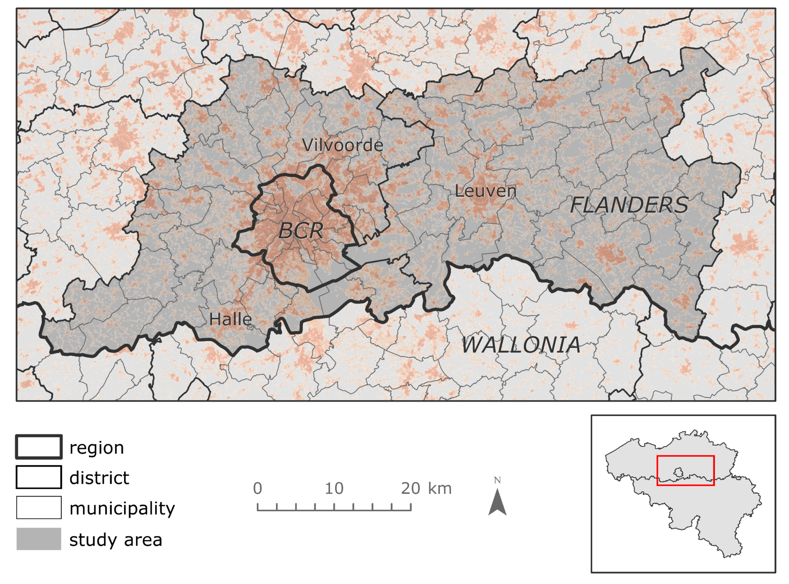
Figure 1. The study area of this research entailing the districts of the Brussels Capital Region (BCR), Halle-Vilvoorde and Leuven, located in the centre of Belgium. Sealed surface density from the European Settlement Layer is added for visual support.
Sustainability 12 02370 g001
Figure 2. A diagram illustrating the time frame and spatial scale of the two residential microsimulation experiments of this research. Secondary analyses were performed to support residential microsimulation.
Sustainability 12 02370 g002
Figure 3. Schematic overview of a simulation year.
Sustainability 12 02370 g003
Figure 4. Observed relocation frequencies between 2003 and 2004, per household segment.
Sustainability 12 02370 g004
Figure 5. Access to public transport (PT) and services, according to [62], and the locations of railway stations.
Sustainability 12 02370 g005
Figure 6. Decision trees used to define residential constraints for the SUS and BAU scenarios.
Sustainability 12 02370 g006
Figure 7. Validation scatterplots of microsimulation results per household segment, plotting simulated versus observed changes in number of households on municipality level between 2001 and 2011. SEI values quantifying the extent to which the point cloud corresponds to the 1:1 line, are added to each scatterplot. The red dotted line on these plots represents the 1:1 line. Additionally, the absolute value of the relative error is displayed for each observation. Dots with red edges correspond to the municipality of Leuven. Dots with blue edges correspond to the municipalities of the Brussels Capital Region.
Sustainability 12 02370 g007
Figure 8. Comparison of SEI values obtained with the proposed simulation model, both uncorrected and corrected for outlier errors, and when performing simulation with a uniform utility model (random).
Sustainability 12 02370 g008
Figure 9. Simulated 2011–2040 change in household density for the SUS and BAU scenarios, mapped on a statistical ward level.
Sustainability 12 02370 g009
Figure 10. Household density difference between the 2040 SUS and BAU microsimulation output (SUS minus BAU). Blue means more in BAU, orange/red means more in SUS.
Sustainability 12 02370 g010
Figure 11. Simulated 2011–2040 household density change for the SUS and BAU urban planning scenarios, mapped for different groupings of household segments on ward level. RP = reference person, HE = higher education.
Sustainability 12 02370 g011
Figure 12. Access to services/public transport (normalized index, see [62]) for the 2011–2040 change in households obtained with the BAU and SUS urban planning scenarios.
Sustainability 12 02370 g012
Figure 13. Comparison between scenario-based microsimulation output, expressed as change in number of households between 2011 and 2035, to the Study Department of the Flemish Government (SVR) projections for the Flemish municipalities of the study area.
Sustainability 12 02370 g013
Table 1. Data used in this study.
DataName Dataset (Publisher)
BrusselsFlanders
Household location and featuresCensus 2001 and 2011 (Statistics Belgium)
Demographic projectionsHPROM (Federal Planning Bureau and Statistics Belgium)
Employment potentialCBE Open Data (Crossroads Bank for Enterprises), Federal Inquiry on Commuting 2011 (FPS Mobility and Transport), (National Social Security Office), Central Reference Address Database (Flanders Information Agency)
Residential relocations 2003-2004(Statistics Belgium)
Access to public transportNode value (Flemish Planning Bureau for the Environment and Spatial Development)
Access to servicesAccess to services (Flemish Planning Bureau for the Environment and Spatial Development)
House selling priceAverage selling price of ordinary houses (Statistics Belgium)
Social housing(Brussels Institute for Statistics and Analysis)(Flemish Society for Social Housing)
Parcels(Land Registry Office)
Buildings(Land Registry Office)
Dwellings per sector in 2001 and 2011Census 2011 (Statistics Belgium)
ZoningDemographic Regional Zoning Map (Perspective.Brussels)Spatial accounting (Spatial Development Department Flanders)
Highway rampsUrbis (Brussels Regional Informatics Centre)
Number of travelers per railway stationiRAIL (National Railway Company of Belgium)
Metro stationsUrbis (Brussels Regional Informatics Centre)n/a
Flood hazardFlood hazard map (Brussels Environment)Flood-prone areas (Coordination Committee on Integrated Water Policy)
Ecologic valueBiologic valuation map
(Research Institute for Nature and Forest)
Table 2. Household segmentation used to perform residential microsimulation. The variables used to construct this segmentation were derived from Census data, of which some relate to a reference person of a household.
AgeChildrenHome OwnershipHighest DegreeSegment2001 Count2011 Count
< 60 yearsYesOwnHigher education (H)180,51395,202
Primary/Second (P/S)2113,03198,917
RentH326,69334,580
P/S470,39994,143
NoOwnH548,59058,055
P/S672,94162,698
RentH783,62095,905
P/S8120,379151,192
>= 60 yearsOwnH934,06849,159
P/S10153,367146,642
RentH11915114,487
P/S1272,94679,721
Total885,698980,701
Table 3. Location features defined on a statistical ward level used to construct location utility and choice models.
Static features
Distance to nearest highway entrance/exit
Access to services
% attached single dwelling houses or apartments
% social housing (defined on municipality level)
Average house selling price (defined on municipality level)
Job density
Employment potential (i.e., jobs within 5km)
Dynamic features
Household density
% households owning their dwelling
% households with children
% households with reference person younger than 60 years
% households with reference person having a higher education degree