Storage of Soil Organic Carbon and Its Spatial Variability in an Agro-Pastoral Ecotone of Northern China

Abstract

Spatial distribution of soil organic carbon (SOC) is important for the development of ecosystem carbon cycle models and assessment of soil quality. In this study, a total of 732 soil samples from 122 soil profiles (0–10, 10–20, 20–40, 40–60, 60–80, and 80–100 cm) were collected by a combination of fixed-point sampling and route surveys in an agro-pastoral ecotone of northern China and the spatial variation of the SOC in the samples was analyzed through classical statistical and geostatistical approaches. The results showed that the SOC contents decreased from 4.31 g/kg in the 0–10 cm to 1.57 g/kg in the 80–100 cm soil layer. The spatial heterogeneity of the SOC exhibited moderate and strong dependence for all the soil layers owing to random and structural factors including soil texture, topography, and human activities. The spatial distributions of the SOC increased gradually from northeast to southwest in the 0–40 cm soil layers, but there was no general trend in deep soil layers and different interpolation methods resulted in the inconsistent spatial distribution of SOC. The storage of SOC was expected to be 25 Tg in the 0–100 cm soil depths for the whole area of 7692 km². The SOC stocks estimated by two interpolation approaches were very close (25.65 vs. 25.86 Tg), but the inverse distance weighting (IDW) interpolation generated a more detailed map of SOC and with higher determination coefficient (R²); therefore, the IDW was recognized as an appropriate method to investigate the spatial variability of SOC in this region.

1. Introduction

Soil organic carbon (SOC) plays an important role in global C cycling, which is sensitive to climate change and anthropogenic disturbance; SOC is roughly comparable to the sum of the atmospheric (750 Pg) and biotic (600 Pg) pools of carbon [1,2], and thus small changes in SOC can greatly alter atmospheric CO₂ concentrations and impact climate change. Understanding the spatial variability and storage of SOC is fundamental for assessing soil fertility, productivity, and C sequestration or emission potential, and establishing land management measures [3,4]. However, accurate estimation of SOC storage is not easy because it is determined by various factors including climatic variables [5], parent materials [6], topography [7], vegetation types [8], soil texture and land use [9], together with significant spatial heterogeneity.

In recent decades, a great number of studies have investigated the storage and distribution of SOC at regional [10], national, and global scales [11,12] using classical statistical and geostatistical approaches. Results showed that the ordinary kriging (OK) interpolation of SOC in Masson pine forests is better than the inverse distance weighting (IDW) method for soil chemical properties in subtropical China [13] and in the district of Tripura, India [14], while the co-kriging method is optimal for SOC estimates in Damavand rangelands, northeast of Teran, within the same spatial scales [15]. These suggest that there is large uncertainty in the estimation of SOC storage due to the different estimation methods and sampling data sets. In fact, to further improve prediction accuracy, numerous new techniques have been applied in the creation of digital soil maps, including random forest, geographically weighted regression [16], and multifactor weighted regression [17]. For example, Tomislav et al. [18] created a global three-dimensional (3D) digital soil map products at 250 m resolution based on machine learning; Liang et al. [19] produced the 3D spatial modeling of SOC maps of China at 90 × 90 m resolution with gradient boosting machines. Schillaci et al. [20] concluded that the integration of soil data with auxiliary variables can also improve the predictive precision of SOC stocks compared to models without auxiliary variables. Moreover, the carbon storage percentage is higher with the increasing soil profile depth from the soil surface in three major soil series of peat soils of Bangladesh [21], but less research focused on SOC stock at deeper soil in other ecosystems [22]. Accordingly, it is crucial to select suitable interpolation approaches to improve our knowledge of SOC stock in 100 cm deep soil layers, which is also the key to estimate the carbon sequestration and its response to climate change in different regions and ecosystems.

The agro-pastoral ecotone in northern China is not only an ecologically fragile transition zone but also a vital ecological barrier to the agriculture zone [23]. The region is extremely vulnerable to soil erosion, grazing, over-cultivation, and human-induced land use, leading to serious land degradation and desertification [24,25]. Moreover, this large area is very sensitive to climate change [26] and has a high potential for sequestering carbon [27,28]. Land use change, grazing exclusion, and afforestation have been shown to increase carbon sequestration in desertified areas [29,30,31]. However, the spatial distribution of SOC storage to a depth of 100 cm has not been reported in this region, which limits our knowledge about SOC sequestration status, temporal changes, and its response to climate change and human disturbance in the future.

To achieve an accurate prediction of the storage and distribution of SOC in a typical agro-pastoral ecotone, we conducted a regional investigation of SOC content through fixed-point sampling and spatial grid approaches. Our specific objectives were to (1) illustrate the spatial variability in soil organic carbon content at 0–10, 10–20, 20–40, 40–60, 60–80, and 80–100 cm soil depths in an agro-pastoral ecotone; (2) compare the spatial distribution patterns derived from IDW and OK interpolation; and (3) estimate the storage of SOC in the whole region.

2. Materials and Methods

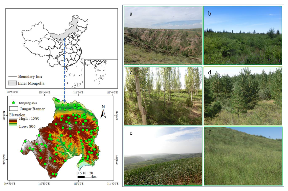
2.1. Study Area

A field survey was conducted in Jungar Banner (39°20′–40°20′ N, 110°13′–111°46′ E) located in the mid-western part of Inner Mongolia, China (Figure 1) with an area of 7692 km², and an elevation ranging from 820 to 1585 m. The area is characterized by a semiarid continental monsoon climate, with a mean annual temperature of 6.7 °C and a mean annual precipitation of 400 mm (with 80% falling from June to September). From the north to the south of the study area, the soil types can be classified into aeolian sandy soil, weathered feldspathic sandstone (Pisha sandstone soil), and loess soil, according to the Food and Agriculture Organization of the United Nations (FAO) classification [32]. The main land use types throughout the region include native grassland (Artemisia ordosica, Stipa grandis, Agropyron cristatum, Lespedeza davurica, Artemisia sacrorum, Stipa bungeana, Caragana microphylla, and Artemisia giraldii Pamp.), artificial forestland (Pinus tabuliformis, Platycladus orientalis, Ulmus pumila L., and Populus alba), shrubland (Caragana korshinskii and Hippophae rhamnoides), and cropland (Solanum tuberosum and maize). The vegetation conversion from cropland to grassland and forestland, or grassland to forestland was started in the 1960s, which included many revegetation types and periods.

2.2. Soil Sampling and Analysis

From July to September 2017, based on information on terrain conditions, land use types, and accessibility, a total of 122 representative sampling sites were determined in the major landscape units (Figure 1), including agricultural land, forestland, grassland, and shrubland. In each sampling site, one 10 m × 10 m plot was established. Soil samples were randomly collected from five sampling points in each plot with a soil auger (5 cm in diameter). The soil profile was divided into six different layers (0–10, 10–20, 20–40, 40–60, 60–80, and 80–100 cm) in each plot, and the soil samples from the same depth were mixed to obtain one composite sample. In addition, one undisturbed soil sample was collected using a soil auger equipped with a stainless-steel cylinder (5.5 cm in diameter and 4.2 cm in height) and the bulk density was determined by drying at 105 °C to a constant mass [33]. The geographic information (elevation, longitude, and latitude) of each sample site was simultaneously recorded with a portable global positioning system (GPS). All the disturbed soil samples were air-dried, ground, and passed through a 0.25 mm sieve for measurement of the SOC content. The SOC content was measured using the K₂Cr₂O₇–H₂SO₄ wet oxidation method [13]. The SOCD and SOCS in each soil layer were calculated using the following equations (Equations (1) and (2)):

$$SOCD =SOC\times BD\times D\times (1-\theta )\times 0.01,$$

(1)

$$SOCS={{\displaystyle \sum }}_{i=1}^n\frac{SOCD\times S}{1000},$$

(2)

where SOCD is the soil organic carbon density (kg/m²), SOCS represents the storage of soil organic carbon (Tg), SOC refers to the soil organic carbon concentration (g/kg) for a certain depth, BD represents the soil bulk density (g/cm³), D is the thickness of the soil depth (cm), θ represents the volumetric percentage of the coarse gravel, 0.01 is the unit conversation factor, S represents the area of pixels in the interpolated SOC map (km²), and n and i are the soil layer.

2.3. Data Analysis

The descriptive statistical analysis for the SOC content was performed using SPSS ver. 20.0 (IBM Corp., Armonk, NY, USA), and the mean, minimum, maximum, standard deviation (SD), coefficient of variation (CV), kurtosis, and skewness values of the SOC content were calculated for each depth. Pearson’s correlation analysis was performed to determine the relationships among the soil properties and sample geographic information.

Geostatistical methods were applied to describe and predict the spatial heterogeneity of the soil properties. The original data set was analyzed with a Kolmogorov–Smirnov test (p < 0.05) to determine whether the soil property data met the assumption of normality for the geostatistical analysis. If the data did not fit a normal distribution (p > 0.05), they were log transformed and then tested for normality. In this study, a semi-variogram was constructed to describe the variability in the SOC concentration by geostatistical software (GS+, ver. 9.0, Tetoc, Beijing, China), including four models (linear, exponential, spherical, and Gaussian) [34]. The model with the smallest residual sum of squares (RSS) and the largest coefficient of determination (R²) had the best performance [35]. The parameters of the semi-variogram model (nugget variance (C₀), structural variance (C), sill variance (C₀ + C) and the spatial autocorrelation range) were used to determine the spatial structure of the SOC at a given scale. The ratio of nugget to sill variance (C₀/(C₀ + C)) was calculated to evaluate the degree of spatial dependence; here, a ratio of <0.25 represents a strong degree of spatial autocorrelation; 0.25–0.75, medium autocorrelation; and >0.75, weak autocorrelation [34,36]. The semi-variogram model was calculated as follows (Equation (3)) [37]:

$$\gamma \left(h\right)=\frac{1}{2N\left(h\right)}{\displaystyle \sum }_1^{N\left(h\right)}{\left[z\left(xi\right)-z\left(xi+h\right)\right]}^2,$$

(3)

where γ(h) is the experimental semi-variogram, h represents the lag distance, N(h) is the number of sampling point pairs with a distance of h, and z (xi) and z (xi + h) are the paired data values with a lag distance of h.

In this study, inverse distance weighting (IDW) and ordinary kriging (OK) interpolation methods were used to describe the spatial distribution of the SOC concentrations. The interpolation performance was tested by a leave-one-out cross-validation approach. The root mean square error (RMSE), mean error (ME), absolute mean error (AME), and determination coefficient (R²) were used to determine the prediction accuracy of the spatial interpolation as follows (Equations (4)–(7)) [35,38]:

$$\mathrm{RMSE}=\sqrt{\frac{1}{n}{{\displaystyle \sum }}_{i=1}^n{(Pi-Mi)}^2},$$

(4)

$$\mathrm{ME}=\frac{1}{n}{{\displaystyle \sum }}_{i=1}^n(Pi-Mi),$$

(5)

$$\mathrm{AME}=\frac{1}{n}{{\displaystyle \sum }}_{i=1}^n\left|\right(Pi-Mi\left)\right|,$$

(6)

$${\mathrm{R}}^2=1-\frac{{{\displaystyle \sum }}_{i=1}^n{\left(Pi-\overline{M}\right)}^2}{{{\displaystyle \sum }}_{i=1}^n{\left(Mi-\overline{M}\right)}^2},$$

(7)

where Pi and Mi represent the predicted measured values, respectively; $\overline{M}$ and $\overline{P}$ are the average of measured and predicted values; and n is the number of sampling points.

All the selected interpolation methods and the creation of the distribution maps were performed in ArcMap ver. 10.2 (ESRI Inc., Redlands, CA, USA) software.

3. Results and Discussion

3.1. Classical Statistical Analysis of Soil Organic Carbon

The mean values of SOC across the entire area significantly decreased with increasing soil depth, ranging from 4.31 g/kg in the 0–10 cm layer to 1.85 g/kg in the 80–100 cm layer (

Table 1. Classical statistical analyses of soil organic carbon concentrations (g/kg) in 0–10, 10–20, 20–40, 40–60, 60–80, and 80–100 cm soil layers.

Depths	Number	Minimum	Maximum	Mean ± SD	CV (%)	Skewness	Kurtosis	K-S	Distribution
0–10 cm	122	1.05	8.35	4.31 ± 1.72	39.80	0.39	−0.43	0.41	Normal
10–20 cm	122	0.72	6.39	3.01 ± 1.24	40.83	0.45	−0.15	0.56	Normal
20–40 cm	122	0.46	4.87	2.32 ± 0.97	41.81	0.39	−0.07	0.88	Normal
40–60 cm	122	0.35	5.57	1.99 ± 0.92	46.20	0.84	1.40	0.50	Normal
60–80 cm	122	0.37	5.36	1.85 ± 0.85	45.78	0.96	2.08	0.36	Normal
80–100 cm	122	0.36	3.93	1.75 ± 0.78	44.05	0.79	0.28	0.10	Normal
0–100 cm	122	0.75	4.54	2.51 ± 0.82	32.68	0.58	−0.628	0.69	Normal

N: number of samples; Min: minimum; Max: maximum; SD: standard deviation; and CV: coefficient of variation.

). This vertical distribution pattern of the SOC was consistent with the results of previous studies from a mountain-basin system in Xinjiang [39] and a catchment in the Loess Plateau, China [40], which resulted from a strong accumulation of organic materials from litter, roots, and microbes at the surface. Compared with the mean value of SOC in China as a whole, the soil organic carbon content was relatively low [7,9], which was attributed to the low productivity, serious land degradation, and desertification in the desert steppe transition zone with a semi-arid climate [41,42]. The coefficients of variation (CV) in SOC varied from 39% to 46%, showing moderate variability [43], which depended largely on the changes in climate, soil texture, pedogenic processes, and land use types [44] (Table 1). The SOC content in loess soil and Pisha sandstone soil was higher than that in Aeolian sandy soil, and it was also higher in grassland and cropland than in forestland due to the great biomass productivity of grassland and the fertilization activities on agricultural land (Supplementary Materials, Figure S1). The Kolmogorov–Smirnov (K-S) test, skewness, and kurtosis values showed that the SOC contents for all the soil layers were consistent with a normal distribution (K-S, p > 0.05; Table 1); therefore, the geostatistical analysis was performed.

3.2. Semi-Variogram Analysis of Soil Organic Carbon

Although the classical statistical analyses adequately reveal the fundamental characteristics of the variation in SOC content, they cannot describe the spatial variation in SOC. Therefore, we performed experimental semi-variogram analyses of the SOC using GS+ software. The results showed that the semi-variograms were best fitted by a spherical model, which had the lowest root square error (RSE) values and the highest determination coefficient (R²). The exception was the 20–40 cm soil layer, for which a Gaussian model provided the best fit (Figure 2,

Table 2. Experimental semi-variogram parameters for the soil organic carbon concentration in the 0–10, 10–20, 20–40, 40–60, 60–80, and 80–100 cm soil layers.

Depths	Model	Nugget (C0)	Sill (C0 + C)	Nugget/Sill (C0/C0 + C)	Spatial Class	Range (m)	R2
0–10 cm	Spherical	0.90	2.52	0.36	moderate	13,831	0.54
10–20 cm	Spherical	0.54	1.36	0.40	moderate	16,205	0.53
20–40 cm	Gaussian	0.20	0.79	0.25	strong	20,929	0.39
40–60 cm	Spherical	0.15	0.76	0.20	strong	18,999	0.25
60–80 cm	Spherical	0.11	0.69	0.16	strong	18,686	0.28
80–100 cm	Spherical	0.15	0.58	0.24	strong	18,693	0.20
0–100 cm	Spherical	0.34	0.66	0.51	moderate	10,616	0.45

C₀: nugget variance; C: structural variance; C₀ + C: sill variance.

) [45]. The ratios of the nugget to the sill were 36% and 40% at depths of 0–10 and 10–20 cm, respectively, while this value was less than 25% in the other soil layers, implying that the SOC had moderate spatial dependence at depths of 0–10 and 10–20 cm but strong spatial dependence in the other soil layers [46]. Previous studies showed that the strong spatial dependence of the soil variables (C₀/(C₀ + C) < 25%) was controlled by intrinsic factors, such as topography, soil texture, and parent material, while the moderate spatial dependence (25% < C₀/(C₀ + C) < 75%) was synchronously affected by intrinsic and extrinsic factors, including not only soil texture, parent material, and topography but also land use management, fertilization, and cultivation practices [34,35,47,48]. For example, the SOC content showed positive correlation with silt, clay, and elevation, and negative correlation with sand (Supplementary Materials, Figure S2). Furthermore, because the significant differences in SOC among vegetation and soil types mainly occurred in the surface soil (Supplementary Materials, Figure S1), it is concluded that the spatial heterogeneity of the SOC in the 0–10 and 10–20 cm layers in our study mainly resulted from the coarse soil texture, severe desertification, and cultivation activities, while in the other soil layers, it resulted from the soil parent material and texture. The nugget to sill ratios showed a decreasing trend with increasing soil depth, which indicated that the spatial heterogeneity of the SOC derived from human activities may be gradually reduced across the soil profile. The spatial range reflects the maximum distance of the spatial autocorrelation for the soil characteristics influenced by environmental factors [49]. In our study, the ranges of the SOC (13.8–20.9 km) were all much larger than the mean distance between the sampling sites (8 km), which indicated that our sampling strategy was suitable for exploring the spatial patterns of SOC in this region [35]. However, the distance between the sampling points was quite widely separated in the southern Loess area with hills and gullies due to poor transportation, which might result in an increase in the spatial range (Figure 1). In addition, the spatial range of the SOC content in the 0–10 cm layer was significantly smaller than those in the other soil layers, indicating that the spatial heterogeneity of the SOC content in the 0–10 cm layer was stronger than those in the other soil layers. Therefore, more sampling points in the 0–10 cm layers should be established to assess the sampling strategy, especially in areas with hills and gullies.

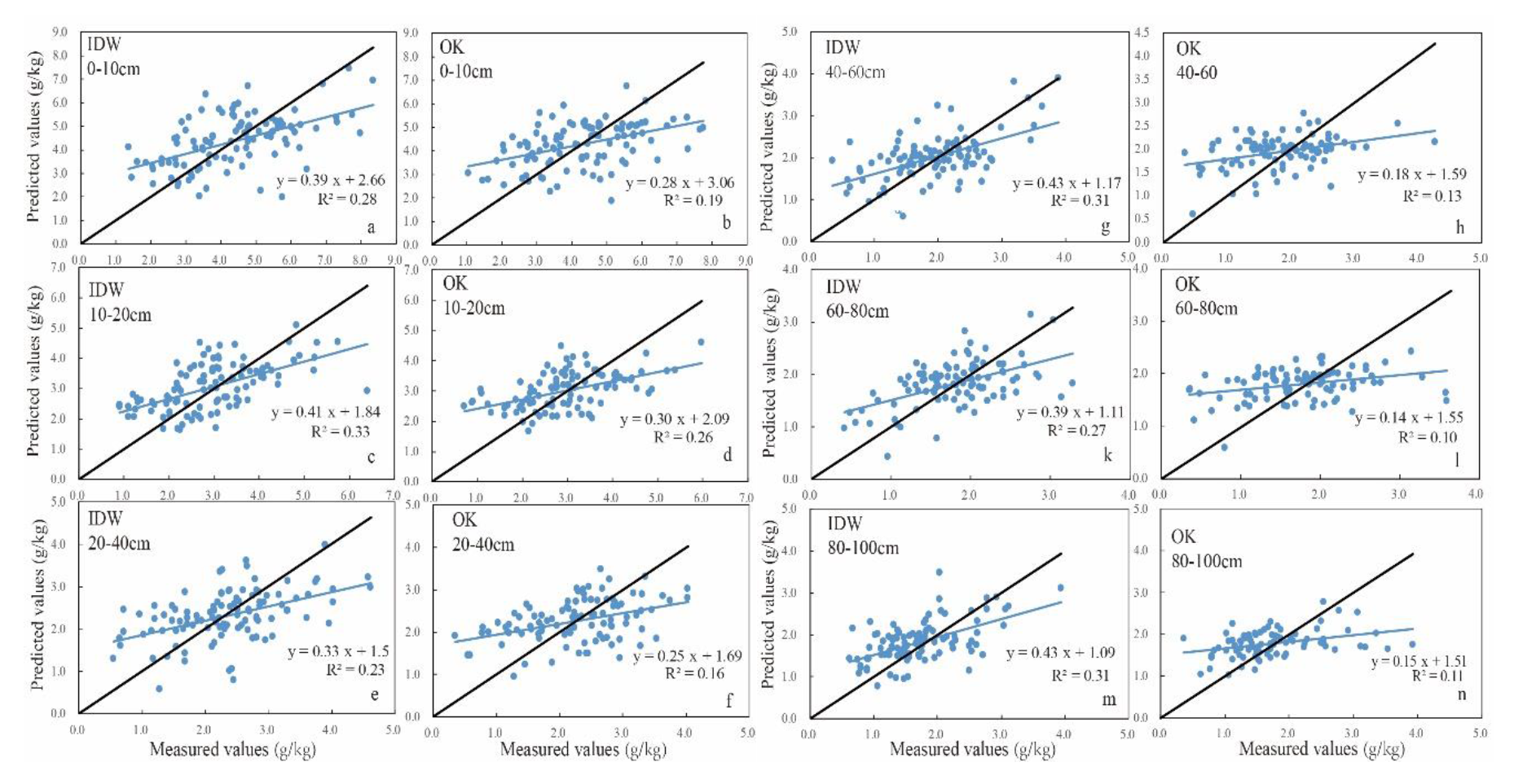
3.3. Spatial Distribution of Soil Organic Carbon Obtained by Interpolation

To further reveal the spatial variability in the SOC, spatial distribution maps of the SOC content were drawn with inverse distance weighting (IDW) and ordinary kriging (OK) interpolation approaches. Overall, the SOC contents throughout the study area in the 0–10, 10–20, and 20–40 cm layers showed similar spatial patterns, which increased gradually from the northern desertified district to the southern area with hills and gullies, i.e., they increased with latitude decrease (Supplementary Materials, Figure S2). Generally, SOC is affected by soil texture, topography, elevation, and climatic factors [50]. In the present study, there was no obvious difference in precipitation throughout the study area; however, the water-holding capacity in the southern areas with hills and gullies dominated by loess soil was higher than that in the northern desertified areas dominated by sandy soil [51]. Considering the positive response of plant biomass to soil moisture [52] and vegetation restoration, the accumulation of SOC generated by litter and roots was more significant in Loess gully region with higher elevation gradient, which could be explained by the positive correlation between SOC and elevation (Supplementary Materials, Figure S2). Moreover, the decomposition of the SOC was associated with soil texture, namely, the physical protection by aggregates of SOC mainly occurred in loess dominated by fine fractions [53]. In summary, the different output and input of organic matter determined by both vegetation and texture could well explain the spatial distribution pattern of the SOC. It is noteworthy that the eastern populous and wealthy region also presented high SOC, which was attributable to the early adoption of vegetation restoration in this region. For the other soil layers, the spatial distributions of the SOC differed significantly among the soil depths, especially between interpolation approaches, but the threshold of SOC content was small.

In particular, the interpolation maps generated by IDW showed detailed divisions, with numerous circular patches around the sampling points for all the soil layers, whereas those generated by OK were characterized by several large modules connected by a continuous curve, especially at 40–60, 60–80, and 80–100 cm soil depths, and the SOC contents were concentrated in a very small range (Figure 3). These differences could be explained by the nature of the interpolation approaches; specifically, OK, which uses a smoothing effect, disregarded those points with the highest or lowest SOC content, while IDW generated patches with a pattern similar to a “bull’s eyes” in some of those points [54]. These spatial distribution patterns supported the previous viewpoint that more samples should be allocated in the surface layer and in the regions with hills and gullies.

To assess the performance of the interpolation methods, cross-validation indices: mean error (ME), root mean square error (RMSE), and absolute mean error (AME) were calculated (

Table 3. Cross-validation indices for the inverse distance weighting (IDW) and ordinary kriging (OK) interpolation methods for determining the soil organic carbon (SOC) contents in the 0–10, 10–20, 20–40 40–60, 60–80, and 80–100 cm soil layers.

	ME		RMSE		AME		R2
Depths (cm)	IDW	OK	IDW	OK	IDW	OK	IDW	OK
0–10 cm	−0.01	−0.02	1.31	1.33	1.04	1.10	28%	19%
10–20 cm	0.09	0.03	0.92	0.89	0.78	0.74	33%	26%
20–40 cm	−0.04	0.01	0.76	0.75	0.62	0.65	23%	16%
40–60 cm	0.09	0.07	0.71	0.66	0.54	0.54	31%	13%
60–80 cm	0.01	0.04	0.52	0.65	0.43	0.51	27%	10%
80–100 cm	0.05	0.06	0.56	0.65	0.47	0.51	30%	12%
0–100 cm	0.05	0.06	0.78	0.77	0.60	0.60	22%	21%

ME: mean error; RMSE: root mean square error; AME: absolute mean error; R²: determination coefficient.

). In general, the values of ME, RMSE, and AME were closer to zero, and the predicted values were closer to the measured values [55]. In the present study, the ME values of the SOC content ranged from 0.01 to 0.10, which indicated that the interpolations of the SOC contents using IDW and OK were relatively unbiased. Although there were no significant differences in the RMSE and AME values between the IDW and OK for each soil layer, the R² values of the IDW method were slightly higher than those of the OK method, indicating that the IDW method was superior to the OK method for the spatial interpolation of SOC (Figure 4). The result was inconsistent with those of previous studies in Masson pine forests [13] and Moso bamboo forests [56] but echoed the result of Gotway et al. [57]. These contradictory results may be associated with sampling allocations and the autocorrelation of the soil properties. It has been reported that the R² values of the predicted and measured values were affected by sample density, distribution, and representativeness, as well as validation method [13,56,58]. Therefore, we could attribute the relatively low R² (10%–33%) values in this study to the limited and unevenly distributed sampling points and, especially, to the nature of the leave-one-out cross-validation method. Furthermore, we also found that both interpolation methods resulted in the underestimation of high measured values, and overestimation of low measured values (Figure 4). To determine the uncertainty source of this estimate, we established the regression curve between measured values and predicted values from IDW and OK interpolation across 0–20 and 20–100 cm, respectively (Supplementary Materials, Figure S3). For both interpolations in 0–20 cm soil layers, the data points of forestlands existed more on the left side of Supplementary Materials, Figure S3a,b, but the data points of croplands and grassland were evenly scattered. In 20–100 cm soil layers, the data points of grassland from both interpolations were clustered near the intersection of fit lines. These results indicated that the accuracy of predicted SOC were related to land use types, i.e., the data points of forestlands would lead to an overestimation of SOC in 0–20 cm soil layer, and the data points of grasslands and forestlands were well predicted by IDW and OK methods in 20–100 cm soil layer. So, the area of different land use types should be considered to improve the estimation accuracy of SOC in the future study.

3.4. Estimation of SOC Storage

The storage of SOC estimated by the IDW and OK methods is presented in

Table 4. Estimation of soil organic carbon (SOC) storage with inverse distance weighted (IDW) and ordinary kriging (OK) interpolation methods.

Depths (cm)	0–10	10–20	20–40	40–60	60–80	80–100	0–100
IDW (Tg)	4.57 ± 0.96	3.23 ± 0.70	5.31 ± 1.22	4.46 ± 1.02	4.20 ± 0.89	3.87 ± 0.80	25.65
OK (Tg)	4.49 ± 0.80	3.33 ± 0.55	5.33 ± 0.93	4.54 ± 0.60	4.22 ± 0.49	3.96 ± 0.40	25.86

. The estimations of SOC storage did not differ between the IDW and OK methods in any soil layer, but they decreased with increasing soil depth. These findings were supported by observations from Masson pine forests in subtropical China [13], which were predominantly determined by the concentrations of SOC and the soil layer interval [13,58,59]. The study area covered 12% of the land area in the Loess Plateau, but the accumulation of stored SOC predicted by the IDW (ca 25.65 Tg) and OK (ca 25.86 Tg) methods accounted for only approximately 0.54% of the total SOC storage in the 0–100 cm layers in the Loess Plateau [60], indicating that both interpolation methods were suitable to estimate the storage of SOC and that the study area had considerable potential for carbon sequestration. In our study, approximately 70% of the SOC was stored in the 0–60 cm soil layers, which was consistent with a study conducted in the Horqin Grassland of northern China [28]. Furthermore, topography can indirectly affect SOC content by changing temperature and precipitation patterns [47,59], which may result in the overestimation or underestimation of SOC storage in the southern hills and gullies area with low sampling density. Considering the high organic carbon content and its sensitivity to climate change and human disturbance in surface soils [28,40,60], we should allocate more sampling sites in the 0–60 cm soil layers while appropriately reducing sampling sites in the other soil layers, thus improving the estimation accuracy of SOC in similar ecosystems with relatively little funding and human resources.

4. Conclusions

The current status and spatial variability of SOC were investigated using a combination of geostatistical and classical statistical methods in an agro-pastoral ecotone of northern China. The region had low SOC content compared with the mean SOC content in China. The contents of SOC for all the soil layers showed moderate or strong spatial dependence, which could be well fitted by exponential or spherical models. The spatial distributions of SOC derived from IDW and OK had similar patterns, with a declining trend from the southwest to the northeast, but the interpolation maps derived from IDW were characterized by small patches, and those from OK were smoother. The storage of SOC across the entire soil profile (0–100 cm) throughout the study area calculated by both interpolation approaches was close to 25 Tg; the 0–60 cm soil layers accounted for approximately 70% of the total storage. These results enriched our knowledge of the current status and distribution of SOC at the regional scale and provided valuable information for verifying how SOC will respond to future climate change and human disturbance. The influential factors, including vegetation index, topography, and meteorological factors should be taken into account to improve the prediction accuracy of SOC in further studies.

References

1. Lal, R. Soils as Source and Sink of Environmental Carbon Diozide. In International Symposium of Molecular Environmental Soil Science at the Interfaces in the Earths Critical Zone; Springer: Berlin/Heidelberg, Germany, 2009. [Google Scholar]
2. Tian, H.; Melillo, J.M.; Kicklighter, D.W.; Mcguire, A.D.; Iii, B.M.; Vörösmarty, C.J. Climatic and biotic controls on annual carbon storage in Amazonian ecosystems. Glob. Ecol. Biogeogr. 2000, 9, 315–335. [Google Scholar] [CrossRef] [Green Version]
3. Wiesmeier, M.; Spörlein, P.; Geuß, U.; Hangen, E.; Haug, S.; Reischl, A.; Schilling, B.; Lützow, M.; Kögel-Knabner, I. Soil organic carbon stocks in southeast Germany (Bavaria) as affected by land use, soil type and sampling depth. Glob. Chang. Biol. 2012, 18, 2233–2245. [Google Scholar] [CrossRef]
4. Wang, S.; Zhuang, Q.; Jia, S.; Jin, X.; Wang, Q. Spatial variations of soil organic carbon stocks in a coastal hilly area of China. Geoderma 2018, 314, 8–19. [Google Scholar] [CrossRef]
5. Zhou, Y.; Hartemink, A.E.; Shi, Z.; Liang, Z.; Lu, Y. Land use and climate change effects on soil organic carbon in North and Northeast China. Sci. Total Environ. 2019, 647, 1230–1238. [Google Scholar] [CrossRef] [PubMed]
6. Bi, Y.; Cai, S.; Wang, Y.; Xia, Y.; Zhao, X.; Wang, S.; Xing, G. Assessing the viability of soil successive straw biochar amendment based on a five-year column trial with six different soils: Views from crop production, carbon sequestration and net ecosystem economic benefits. J. Environ. Manag. 2019, 245, 173–186. [Google Scholar] [CrossRef]
7. Mao, D.H.; Wang, Z.M.; Li, L.; Miao, Z.H.; Ma, W.H.; Song, C.C.; Ren, C.Y.; Jia, M.M. Soil organic carbon in the Sanjiang Plain of China: Storage, distribution and controlling factors. Biogeosciences 2015, 12, 1635–1645. [Google Scholar] [CrossRef] [Green Version]
8. Shi, Z.; Li, X.; Zhang, L.; Wang, Y. Impacts of farmland conversion to apple (Malus domestica) orchard on soil organic carbon stocks and enzyme activities in a semiarid loess region. J. Plant Nutr. Soil Sci. 2015, 178, 440–451. [Google Scholar] [CrossRef]
9. Nie, X.; Peng, Y.; Li, F.; Yang, L.; Xiong, F.; Li, C.; Zhou, G. Distribution and controlling factors of soil organic carbon storage in the northeast Tibetan shrublands. J. Soil. Sediment. 2019, 19, 322–331. [Google Scholar] [CrossRef]
10. Li, Z.P.; Han, F.X.; Su, Y.; Zhang, T.L.; Sun, B.; Monts, D.L.; Plodinec, M.J. Assessment of soil organic and carbonate carbon storage in China. Geoderma 2007, 138, 119–126. [Google Scholar] [CrossRef]
11. Torn, M.S.; Trumbore, S.E.; Chadwick, O.A.; Vitousek, P.M.; Hendricks, D.M. Mineral control of soil organic carbon storage and turnover. Nature 1997, 389, 170–173. [Google Scholar] [CrossRef]
12. Post, W.M.; Emanuel, W.R.; Zinke, P.J.; Stangenberger, A.G. Soil carbon pools and world life zones. Nature 1982, 298, 156–159. [Google Scholar] [CrossRef]
13. Yao, X.; Yu, K.; Deng, Y.; Zeng, Q.; Lai, Z.; Liu, J. Spatial distribution of soil organic carbon stocks in Masson pine (Pinus massoniana) forests in subtropical China. Catena 2019, 178, 189–198. [Google Scholar] [CrossRef]
14. Jafar, Y.; Saffari, M.; Fathi, H.; Karimian, N.; Moazallahi, M.; Gazni, R. Evaluation and comparison of ordinary kriging and inverse distance weighting methods for prediction of spatial variability of some chemical parameters. Res. J. Biol. Sci. 2009, 4, 93–102. [Google Scholar]
15. Dadgar, M.; Esfahan, E.Z.; Rabiee, M.R.S. Spatial variation of soil organic carbon in damavand rangelands. J. Biodivers. Environ. Sci. 2014, 5, 72–77. [Google Scholar]
16. Wang, S.Z.; Fan, J.W.; Li, Z.H.; Zhu, H.Z.; Qiao, Y.L. A multi-factor weighted regression approach for estimating the spatial distribution of soil organic carbon in grasslands. Catena 2019, 174, 248–258. [Google Scholar] [CrossRef]
17. Wang, D.; Li, X.X.; Zou, D.F.; Wu, T.H.; Hu, G.J.; Li, R.; Ding, Y.L.; Zhao, L.; Wu, X.D. Modeling soil organic carbon spatial distribution for a complex terrain based on geographically weighted regression in the eastern Qinghai-Tibetan Plateau. Catena 2020, 187, 104399. [Google Scholar] [CrossRef]
18. Tomislav, H.; Jorge, M.D.J.; Heuvelink, G.B.M.; Gonzalez1, M.R.; Kilibarda, M.; Blagotić, A.; Wei, S.; Wright, M.N.; Geng, X.Y.; Bauer-Marschallinger, B.; et al. SoilGrids250m: Global gridded soil information based on machine learning. PLoS ONE 2017, 12, e0169748. [Google Scholar] [CrossRef] [Green Version]
19. Liang, Z.Z.; Chen, S.C.; Yang, Y.; Zhou, Y.; Shi, Z. High-resolution three-dimensional mapping of soil organic carbon in China: Effects of SoilGrids products on national modeling. Sci. Total Environ. 2019, 685, 480–489. [Google Scholar] [CrossRef]
20. Schillaci, C.; Acutis, M.; Lombardo, L.; Fantappiè, M.; Märker, M.; Saia, S. Spatio-temporal topsoil organic carbon mapping of a semi-arid Mediterranean region: The role of land use, soil texture, topographic indices and the influence of remote sensing data to modelling. Sci. Total Environ. 2017, 601–602, 821–832. [Google Scholar] [CrossRef]
21. Minasny, B.; Malone, B.P.; McBratney, A.B.; Angers, D.A.; Arrouays, D.; Chambers, A.; Chaplot, V.; Chen, Z.A.; Cheng, K.; Das, B.S.; et al. Soil Carbon 4 Per Mille. Geoderma 2017, 292, 59–86. [Google Scholar] [CrossRef]
22. Chen, S.C.; Martin, M.P.; Saby, N.P.A.; Walter, C.; Angers, D.A.; Arrouays, D. Fine resolution map of top- and subsoil carbon sequestration potential in France. Sci. Total Environ. 2018, 630, 389–400. [Google Scholar] [CrossRef] [PubMed]
23. Zhao, H.L.; Zhao, X.Y.; Zhang, T.H.; Zhou, R.L. Boundary line on agro-pasture zigzag zone in north China and its problems on eco-environment. Adv. Earth Sci. 2002, 17, 739–747. (In Chinese) [Google Scholar]
24. Liu, J.; Chen, H.; Yang, X.; Gong, Y.; Zheng, X.; Fan, M.; Kuzyakov, Y. Annual methane uptake from different land uses in an agro-pastoral ecotone of northern China. Agric. For. Meteorol. 2017, 236, 67–77. [Google Scholar] [CrossRef]
25. Yao, Y.; Ge, N.; Yu, S.; Wei, X.; Wang, X.; Jin, J.; Liu, X.; Shao, M.; Wei, Y.; Kang, L. Response of aggregate associated organic carbon, nitrogen and phosphorous to re-vegetation in agro-pastoral ecotone of northern China. Geoderma 2019, 341, 172–180. [Google Scholar] [CrossRef]
26. Li, S.; An, P.; Pan, Z.; Wang, F.; Li, X.; Liu, Y. Farmers’ initiative on adaptation to climate change in the Northern Agro-pastoral Ecotone. Int. J. Disast. Risk Reduct. 2015, 12, 278–284. [Google Scholar] [CrossRef]
27. Nosetto, M.D.; Jobbagy, E.G.; Paruelo, J.M. Carbon sequestration in semi-arid rangelands: Comparison of Pinus ponderosa plantations and grazing exclusion in NW Patagonia. J. Arid Environ. 2006, 67, 142–156. [Google Scholar] [CrossRef]
28. Li, Y.; Wang, X.; Niu, Y.; Lian, J.; Luo, Y.; Chen, Y.; Gong, X.; Yang, H.; Yu, P. Spatial distribution of soil organic carbon in the ecologically fragile Horqin Grassland of northeastern China. Geoderma 2018, 325, 102–109. [Google Scholar] [CrossRef]
29. Li, Q.; Yang, D.; Jia, Z.; Zhang, L.; Zhang, Y.; Feng, L.; He, L.; Yang, K.; Dai, J.; Chen, J.; et al. Changes in soil organic carbon and total nitrogen stocks along a chronosequence of Caragana intermedia plantations in alpine sandy land. Ecol. Eng. 2019, 133, 53–59. [Google Scholar] [CrossRef]
30. Li, Q.; Zhou, D.; Denton, M.D.; Cong, S. Alfalfa monocultures promote soil organic carbon accumulation to a greater extent than perennial grass monocultures or grass-alfalfa mixtures. Ecol. Eng. 2019, 131, 53–62. [Google Scholar] [CrossRef]
31. Li, Y.; Zhou, X.; Brandle, J.R.; Zhang, T.; Chen, Y.; Han, J. Temporal progress in improving carbon and nitrogen storage by grazing exclosure practice in a degraded land area of China’s Horqin Sandy Grassland. Agric. Ecosyst. Environ. 2012, 159, 55–61. [Google Scholar] [CrossRef]
32. Cui, Y.; Fang, L.; Guo, X.; Wang, X.; Zhang, Y.; Li, P.; Zhang, X. Ecoenzymatic stoichiometry and microbial nutrient limitation in rhizosphere soil in the arid area of the northern Loess Plateau, China. Soil Biol. Biochem. 2018, 116, 11–21. [Google Scholar] [CrossRef]
33. Wei, X.; Li, X.; Jia, X.; Shao, M. Accumulation of soil organic carbon in aggregates after afforestation on abandoned farmland. Biol. Fert. Soils 2012, 49, 637–646. [Google Scholar] [CrossRef]
34. Goovaerts, P. Geostatistics in soil science: State-of-the-art and perspectives. Geoderma 1999, 89, 1–45. [Google Scholar] [CrossRef]
35. Liu, Z.P.; Shao, M.A.; Wang, Y.Q. Spatial patterns of soil total nitrogen and soil total phosphorus across the entire Loess Plateau region of China. Geoderma 2013, 197–198, 67–78. [Google Scholar] [CrossRef]
36. Bruland, G.L.; Grunwald, S.; Osborne, T.Z.; Reddy, K.R.; Newman, S. Spatial Distribution of Soil Properties in Water Conservation Area 3 of the Everglades. Soil Sci. Soc. Am. J. 2006, 70, 1662–1670. [Google Scholar] [CrossRef] [Green Version]
37. Schöning, I.; Totsche, K.U.; Kögel-Knabner, I. Small scale spatial variability of organic carbon stocks in litter and solum of a forested Luvisol. Geofis. Int. 2006, 136, 631–642. [Google Scholar] [CrossRef]
38. Ye, L.; Tan, W.; Fang, L.; Ji, L.; Deng, H. Spatial analysis of soil aggregate stability in a small catchment of the Loess Plateau, China: I. Spatial variability. Soil Tillage Res. 2018, 179, 71–81. [Google Scholar] [CrossRef]
39. Bi, X.; Li, B.; Nan, B.; Fan, Y.; Fu, Q.; Zhang, X. Characteristics of soil organic carbon and total nitrogen under various grassland types along a transect in a mountain-basin system in Xinjiang, China. J. Arid Land 2018, 10, 612–627. [Google Scholar] [CrossRef] [Green Version]
40. Han, F.; Hu, W.; Zheng, J.; Du, F.; Zhang, X. Estimating soil organic carbon storage and distribution in a catchment of Loess Plateau, China. Geoderma 2010, 154, 261–266. [Google Scholar] [CrossRef]
41. Li, C.; Hao, X.; Zhao, M.; Han, G.; Willms, W.D. Influence of historic sheep grazing on vegetation and soil properties of a Desert Steppe in Inner Mongolia. Agric. Ecosyst. Environ. 2008, 128, 109–116. [Google Scholar] [CrossRef]
42. Xu, H.P.; Zhang, J.; Pang, X.P.; Wang, Q.; Zhang, W.N.; Wang, J.; Guo, Z.G. Responses of plant productivity and soil nutrient concentrations to different alpine grassland degradation levels. Environ. Monit. Assess. 2019, 191, 678. [Google Scholar] [CrossRef] [PubMed]
43. Wilding, L.P. Spatial variability: Its documentation, accommodation, and implication to soil surveys. In Soil Spatial Variability; Nielsen, D.R., Bouma, J., Eds.; Pudoc: Wageningen, The Netherlands, 1985; pp. 166–194. [Google Scholar]
44. Tsatskin, A.; Sandler, A.; Porat, N. Toposequence of sandy soils in the northern coastal plain of Israel: Polygenesis and complexity of pedogeomorphic development. Geoderma 2013, 197–198, 87–97. [Google Scholar] [CrossRef]
45. Wang, Y.; Zhang, X.; Huang, C. Spatial variability of soil total nitrogen and soil total phosphorus under different land uses in a small watershed on the Loess Plateau, China. Geoderma 2009, 150, 141–149. [Google Scholar] [CrossRef]
46. Cambardella, C.A.; Moorman, T.B.; Novak, J.M.; Parkin, T.B.; Karlen, D.L.; Turco, R.F.; Konopka, A.E. Field-scale varibility of soil properties in central iowa central iowa soils. Soil Sci. Soc. Am. J. 1994, 58, 1501–1511. [Google Scholar] [CrossRef]
47. Wendroth, O.; Rogasik, H.; Koszinski, S.; Ritsema, C.J.; Dekker, L.W.; Nielsen, D.R. State space prediction of field scale soil water content time series in a sandy loam. Soil Tillage Res. 1999, 50, 85–93. [Google Scholar] [CrossRef]
48. Cambardella, C.A.; Karlen, D.L. Spatial Analysis of Soil Fertility Parameters. Precis. Agric. 1999, 1, 5–14. [Google Scholar] [CrossRef]
49. Abuduwaili, J.; Tang, Y.; Abulimiti, M.; Liu, D.; Ma, L. Spatial distribution of soil moisture, salinity and organic matter in Manas River watershed, Xinjiang, China. J. Arid Land 2012, 4, 441–449. [Google Scholar] [CrossRef]
50. Luo, Z.; Feng, W.; Luo, Y.; Baldock, J.; Wang, E. Soil organic carbon dynamics jointly controlled by climate, carbon inputs, soil properties and soil carbon fractions. Glob. Chang. Biol. 2017, 23, 4430–4439. [Google Scholar] [CrossRef]
51. Zhen, Q.; Zheng, J.; He, H.; Han, F.; Zhang, X. Effects of Pisha sandstone content on solute transport in a sandy soil. Chemosphere 2016, 144, 2214–2220. [Google Scholar] [CrossRef]
52. Zhao, J.X.; Luo, T.X.; Wei, H.X.; Deng, Z.H.; Li, X.; Li, R.C.; Tang, Y.H. Increased precipitation offsets the negative effect of warming on plant biomass and ecosystem respiration in a Tibetan alpine steppe. Agric. For. Meteorol. 2019, 279, 107761. [Google Scholar] [CrossRef]
53. Ge, N.; Wei, X.; Wang, X.; Liu, X.; Shao, M.; Jia, X.; Li, X.; Zhang, Q. Soil texture determines the distribution of aggregate-associated carbon, nitrogen and phosphorous under two contrasting land use types in the Loess Plateau. Catena 2019, 172, 148–157. [Google Scholar] [CrossRef]
54. Bouma, J.; de Vos, J.A.; Sonneveld, M.R.W.; Heuvelink, G.B.M.; Stoorvogel, J.J. The role of scientists in multiscale land use analysis: Lessons learned from Dutch Communities of Practice. Adv. Agron. 2008, 97, 175–237. [Google Scholar]
55. Meersmans, J.; Martin, M.P.; De Ridder, F.; Lacarce, E.; Wetterlind, J.; De Baets, S.; Bas, C.; Louis, B.P.; Orton, T.G.; Bispo, A. A novel soil organic C model using climate, soil type and management data at the national scale in France. Agrono. Sustain. Dev. 2013, 32, 873–888. [Google Scholar] [CrossRef] [Green Version]
56. Tang, X.; Xia, M.; Perez-Cruzado, C.; Guan, F.; Fan, S. Spatial distribution of soil organic carbon stock in Moso bamboo forests in subtropical China. Sci. Rep. 2017, 7, 42640. [Google Scholar] [CrossRef] [PubMed] [Green Version]
57. Gotway, C.A.; Ferguson, R.B.; Hergert, G.W.; Peterson, T.A. Comparison of kriging and inverse-distance methods for mapping soil parameters. Soil Sci. Soc. Am. J. 1996, 60, 1237–1247. [Google Scholar] [CrossRef]
58. Ye, H.; Huang, W.; Huang, S.; Huang, Y.; Zhang, S.; Dong, Y.; Chen, P. Effects of different sampling densities on geographically weighted regression kriging for predicting soil organic carbon. Spat. Stat. 2017, 20, 76–91. [Google Scholar] [CrossRef]
59. Tan, Z.X.; Lal, R.; Smeck, N.E.; Calhoun, F.G. Relationships between surface soil organic carbon pool and site variables. Geoderma 2004, 121, 187–195. [Google Scholar] [CrossRef]
60. Liu, Z.P.; Shao, M.A.; Wang, Y.Q. Effect of environmental factors on regional soil organic carbon stocks across the Loess Plateau region, China. Agric. Ecosyst. Environ. 2011, 142, 184–194. [Google Scholar] [CrossRef]
Figure 1. Geographical location of the study area, sampling sites, and typical landscapes: (a) desolate meadow; (b) shrub land; (c,d) revegetated woodland land; (e) farmland; and (f) revegetated grassland.
Sustainability 12 02259 g001
Figure 2. Semi-variogram charts of the soil organic carbon (SOC) concentration in the 0–10 cm (a), 10–20 cm (b), 20–40 cm (c), 40–60 cm (d), 60–80 cm (e), and 80–100 cm (f) soil layers.
Sustainability 12 02259 g002
Figure 3. Spatial distribution of the soil organic carbon (SOC) contents (g kg−1) in the sub-plots: in the 0–10 cm (a,b); in the 10–20 cm (c,d); in the 20–40 cm (e,f); in the 40–60 cm (g,h), in the 60–80 cm (k,l), and in the 80–100 cm (m,n) soil layers estimated by the inverse distance weighting (IDW) and ordinary kriging (OK) interpolation methods.
Sustainability 12 02259 g003
Figure 4. Cross-validation of inverse distance weighting (IDW) and ordinary kriging (OK) in the 0–10 cm (a,b); in the 10–20 cm (c,d); in the 20–40 cm (e,f); in the 40–60 cm (g,h), in the 60–80 cm (k,l), and in the 80–100 cm (m,n) soil layers (black line represents a 1:1 regression line).
Sustainability 12 02259 g004