Substantiating the Logistics Chain Structure While Servicing the Flow of Requests for Road Transport Deliveries

Abstract

The selection of the delivery scheme is one of the most complicated problems and the results of its solution condition the sustainable development of the whole market of transportation services. Freight forwarders should consider numerous random parameters characterizing demand and technological processes to choose the proper structure of the logistics chain. The paper aims to propose a method for choosing the logistics chain structure, based on the analysis of the total expenses as a function from the demand parameters characterizing stochastic variables of the consignment weight, the delivery distance, and the time interval between the requests in the flow of queries for cargo delivery. Four basic logistics chain structures, widely used on road transport, are described to demonstrate the selection process. The areas of the most efficient use of the logistics chain structures can be defined for the flow of requests for cargo deliveries. The paper shows such areas on the example of goods delivery by automobile transport. Determining the areas of the most efficient use of the specific logistics chain structures contributes to the effective choice of correct delivery variants by freight forwarders.

1. Introduction

The process of cargo delivery is a complex stochastic process, due to the influence of a large number of random factors on technological operations. The processes of interaction between enterprises at the transportation market are organized by freight forwarders, therefore the efficiency of the forwarding technological process fully determines the sustainable development of the transportation market as the macro-logistics system. Selecting the logistics chain structure is one of the main problems being solved by freight forwarders, which ensures minimal expenses of the delivery process participants. The results of this problem-solving process significantly influence the sustainable development of the transportation market as a macro logistics system.

Substantiating the logistics chain structure is usually considered as a part of a more sophisticated task—designing the supply chain. The recent literature describes that task as a complicated procedure involving numerous subtasks at different levels of the decision-making process. The logistics chain represents the successive steps that are being implemented to achieve the process goal whether it is a product manufacturing or goods delivery. In the case of the goods delivery, these steps are defined by the involved transportation market entities and the logistics chain structure can be described by the used delivery scheme as a sequence of these entities. The supply chain is a more complicated system, being defined as the sequence of sub-processes that are related to the production and distribution of goods. However, the logistics chain structure can be considered as the backbone of the supply chain design and a crucial factor defining the supply chain efficiency. Carvalho and Fonseca (2017) state that the proper logistics structure is the key factor of competitiveness [1].

Melnyk et al. (2014) propose a framework of supply chain design that comprehends business and political environment, the supply chain lifecycle, behavioral, and structural design elements that define a supply chain, and technological operations being implemented within a supply chain [2]. Blos et al. (2018), in their framework for the supply chain design, underline that the carrier viewpoint should be considered in the designing process [3]. According to Yao and Askin (2019), the decision-making procedures concerning the product and supply chain design should be jointly developed [4], which increases the design complexity, but might result in the optimal decision. Bányai et al. underline the impact of routing procedures on environmental awareness and sustainability [5] and the influence of the scheduling outcome on energy efficiency [6]. Calleja et al. (2018) provide a review of methodological approaches to supply chain design and conclude that the use of typical solutions for supply chains designing is not the proper approach, while the methods proposing a succession of stages to follow through the design process may be effective if they are clear for practitioners [7]. The facility location is another issue to be considered while designing the supply chain structure [8]; however, in terms of the problem of choosing the logistics chain structure, the location of facilities only influences the constant operational costs used as initial data while solving the problem. A number of authors also pay significant attention to the consideration of the random nature of demand and technological processes [9,10], which results in the appearance of risk factors [11,12,13].

Sustainability issues that are related to the supply chain design problem are widely discussed in the recent scientific literature. Moreno-Camacho et al. (2019) state that increasing pressure from governments and other different groups of stakeholders has motivated the study of sustainability assessment in the supply chain context [14]. Three pillars of the system development, i.e., economic, environmental, and social, should be considered in the process of a supply chain design, according to the sustainable development paradigm. These directions are highlighted in a number of publications that are devoted to the design and implementation of sustainable supply chains [15,16,17,18].

While solving the problems that are related to optimization of the logistics chain structure, the authors use criteria corresponding to the mentioned directions of sustainable development: the authors of the paper [15] propose minimizing the total cost as economic issue, minimizing the total amount of CO₂ emission as environmental issue, and maximizing the total social influence as social issue; Sherafati et al. (2019) maximize profit primarily while capturing social development by prioritizing the less developed regions and dealing with ecological aspect by using environmentally friendly transport facilities [16]. Accordingly, optimization problems that are related to sustainable supply chain design are solved as multi-objective problems [15,16,17,18]. The authors of the paper [14] have analyzed more than 100 papers, including documents studying supply chains, and came up with the conclusion that modern literature emphasizes the environmental aspects of the supply chain design, but does not pay much attention to social criteria. It should be noted that the commonly used efficiency criterion that allows for considering three directions of sustainable development is the total costs, which include all of the losses and expenses related to environmental and social issues [19,20,21].

The optimization methods used in the recent publications vary from certain methods (augmented ε-constraint method [18], robust programming [16]) to the methods, where heuristics should be used to obtain a solution (hybrid genetic algorithm [15], mixed-integer linear programming model [20]).

The current paper contributes to the structural design of the supply chain by defining the optimal (within the given set of alternatives) solution for the delivery scheme. The decision regarding the structure of the logistics chain is being made while considering the viewpoint of all the transport market entities participating in the delivery process; the implications of this decision define the sustainable development of the whole macro-logistics system. Additionally, in the method that was proposed by this paper, the demand parameters are taken into consideration as the characteristics of the flow of requests for transport services. Consequently, the areas of the most efficient use of the delivery schemes can be established for the considered demand parameters. In that way, while choosing the proper structure of the logistics chain, the decision-maker (e.g., freight forwarder) will obtain the answer by applying the consignment parameters as arguments, without implementing the time-consuming procedures of the evaluation of the costs for all the alternative structures.

2. Methodology

The structure of the logistics chain (LC) describes the structure of the technological process of cargo delivery, which reflects the sequence of participants in the delivery process of various entities at the transport services market. It is necessary to distinguish the problem of choosing the optimal LC variant and the problem of substantiating the optimal carrier (an operator, a contractor for performing certain types of work, etc.) or the optimal delivery route. The choice of the LC structure should be justified before making a decision on participation in the delivery process of a specific transportation market entity, since it refers to the task of management at the macro-level.

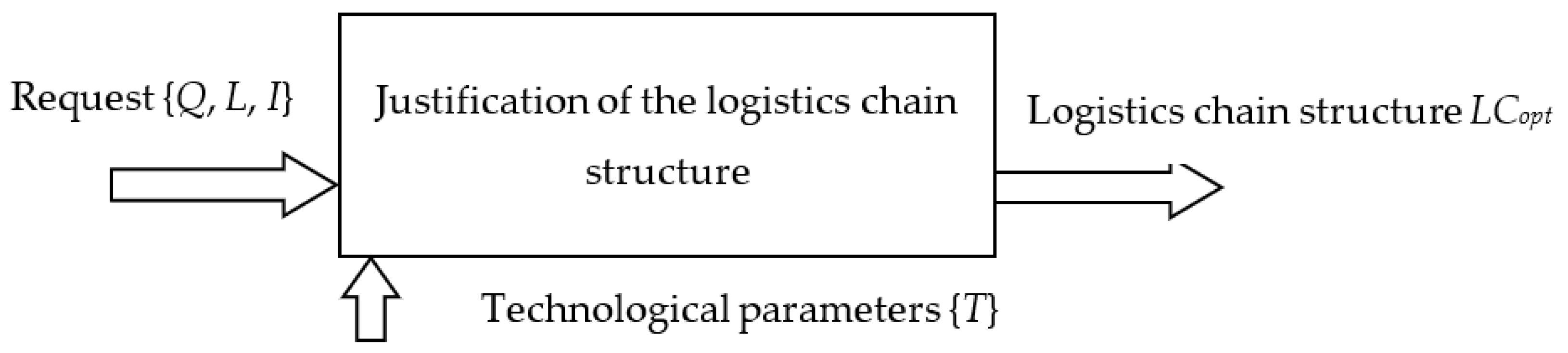
2.1. Problem Statement

Figure 1 presents the process of choosing the optimal LC as a cybernetic model. A set of incoming parameters is described by the numerical characteristics of a request for a consignment for delivery—its weight $Q$, the delivery distance $L$, and the interval $I$ of the request arrival [22,23]. The influence of environmental factors is described by the values of parameters $\left\{T\right\}$, characterizing the technological processes of the LC entities, in the mathematical model, these parameters are realizations of random variables of the delivery speed, the time of specific technological operations, non-production vehicle downtime, etc. The result of the choice is such the structure $L{C}_{opt}$, for which the value of the considered efficiency criterion is optimal.

When solving problems at the macro-logistical level, it is advisable to use the total costs of the entities that form the LC as the efficiency criterion (this indicator is considered as the objective function in [19,20,24,25], and is also used as a sub-criterion in [26,27]). In this case, the problem of choosing the optimal LC structure can be formalized, as follows:

$$L{C}_{opt}=\underset{LC}{\arg }\underset{i}{\min }{E}_{\Sigma i},$$

(1)

where: $E_{\Sigma i}$ is the total costs of entities within the logistics chain.

In this case, the total costs are functionally determined by a set of input parameters and the parameters describing the influence of the external environment:

$$E_{\Sigma }=f\left(LC,\left\{Q,L,I\right\},\left\{T\right\}\right).$$

(2)

Mandatory elements of the LC are the consignor $F{O}^A$ and the consignee $F{O}^B$. The LC also contains at least one forwarder and one carrier. Cargo terminals may also be included in complex LC with the participation of several carriers and freight forwarders. A customs point should be considered in the case of international delivery of goods, as a specific element, the presence of which determines the cost structure for other participants in the supply chain. In general, the LC structure can be formalized, as follows:

$$LC=\left\{F{O}^A;\left\{C\right\};\left\{FT\right\};\left\{FF\right\};F{O}^B;CP\right\},$$

(3)

where $\left\{C\right\}$ is the set of carriers; $\left\{FT\right\}$ is the set of cargo terminals; $\left\{FF\right\}$ is the set of freight forwarders; and, $CP$ is the customs point.

While using the above formulation of the problem, in general, the methodology for selecting the optimal LC structure can be defined as the sequential implementation of three stages:

• The formation of alternative LC variants, determining the structure of the technological scheme. Alternatives are determined on the basis of the availability of cargo terminals, customs points, as well as partner forwarders operating in the appropriate geographic area.
• The efficiency evaluation for a set of alternative structures. The assessment is carried out on the basis of average market value indicators, while taking the random nature of technological parameters into account. The result of the evaluation for each LC variant is a random value of the efficiency criterion.
• The selection of the optimal LC structure and subsequent measures related to the determination of the LC participants and the development of specific technological processes. The choice of the optimal LC structure is carried out on the basis of a comparative assessment of characteristics of random variables that describe the effectiveness criterion for each alternative structure. For the presented formulation of the problem (1), the choice is made according to the minimum expected value of the total costs.

While choosing the optimal LC variant, alternative structures can be preliminarily eliminated if additional preferences of customers in terms of delivery time and quality of service are known.

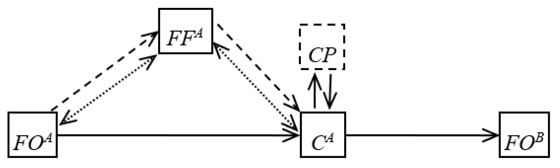
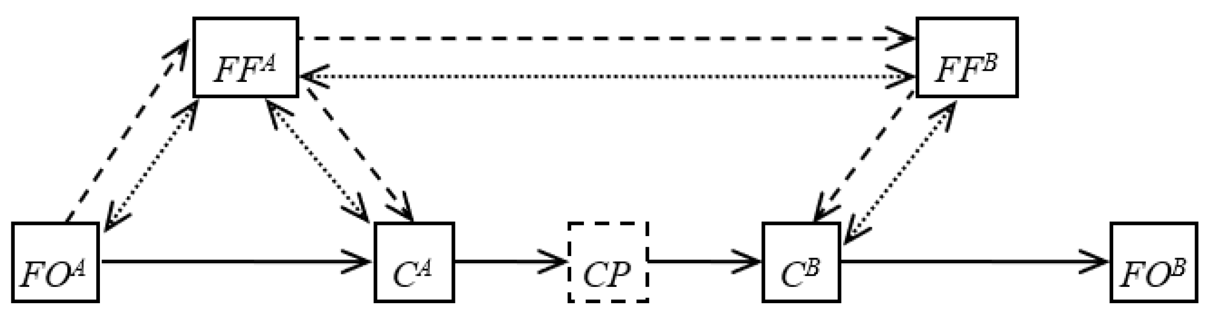
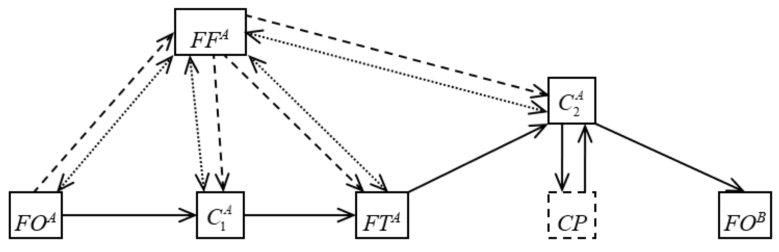
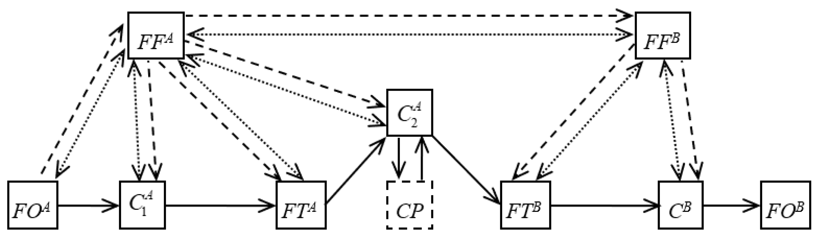
2.2. Basic Alternative Variants of the Logistics Chains’ Structure

The choice of the best LC structures is carried out on a set of alternatives. Let us consider the basic variants of the LC structures for goods delivery by road transport.

For an individual LC as a part of a logistics system, the initial element generating the material flow is the cargo owner (consignor), and the final element is the other cargo owner (consignee). Accordingly, the initial and final elements in the supply chain are freight owners. Physically, a carrier performs the processing of the material flow. The organization of the material flow processing is implemented by a freight forwarder using, if necessary, the resources of cargo terminals. As an organizer of the technological processes, a freight forwarder is an element of LC, which concentrates information flows. Since the freight owner, in order to fulfill his need in goods delivery, addressing the freight forwarder, the cash flow in the LC passes initially from the owner to the freight forwarder, and then to the other participants in the chain.

Figure 2 presents the simplest version of LC. The presence of the $CP$ element in the LC structure is marked by a dotted line, since this element is only present in the case of international delivery of goods.

Formally, the simplest supply chain $L{C}^{1F}$ is a collection of elements of the following type:

$$L{C}^{1F}=\left\{F{O}^A;C^A;F{F}^A;F{O}^B;CP\right\},$$

(4)

where $C^A$ is a carrier in the region of a consignor; and, $F{F}^A$ is a freight forwarder in the region of a consignor.

For this option, the delivery process is coordinated by one forwarder, one carrier is involved in the transportation, and cargo terminals are not involved in the delivery process. The shipper declares his need to relocate the shipment. The freight forwarder determines a carrier who can deliver this consignment to the consignee, and then contacts the shipper, concludes bilateral agreements for arranging delivery between the freight forwarder and the shipper, and also between the freight forwarder and the carrier. The shipper pays the freight forwarder’s services; from the amount that was received from the customer, the freight forwarder pays for the carrier’s services. The carrier delivers a shipment from the shipper to the border, and then from the customs point to the consignee. This version of LC is typical for the delivery of goods by road transport when the consignment weight equals the vehicle capacity.

A more complicated version is the LC variant with the participation of two freight forwarders and, accordingly, of two carriers (Figure 3).

Such a variant of LC ($L{C}^{2F}$-type chain) is the following set of elements:

$$L{C}^{2F}=\left\{F{O}^A;C^A;F{F}^A;F{O}^B;C^B;F{F}^B;CP\right\},$$

(5)

where $C^B$ is a carrier in the region of a consignee; and, $F{F}^B$ is a freight forwarder in the region of a consignee.

After receiving the request from a shipper, a freight forwarder finds a carrier for the delivery of the consignment to the border, and also sends the request to the partner forwarder. The partner forwarder organizes the delivery of a consignment from the border to the consignee, while using a regional carrier. In such a situation, four bilateral agreements are signed: between the freight forwarder and the shipper, between the freight forwarder and the carrier, between two freight forwarders, and also between the foreign freight forwarder and the foreign carrier. In this case, the shipper will pay for the services of the first forwarder, which of the received reward will pay for the services of the regional carrier, as well as the services of the foreign forwarder. A partner forwarder pays for carrier services in his region from the received remuneration.

The cargo terminal is involved in the process of processing the material flow in the LC version that is presented in Figure 4.

This variant of the logistics chain ($L{C}^{1T}$-type chain) is a combination of seven basic elements:

$$L{C}^{1T}=\left\{F{O}^A;C_1^A;C_2^A;F{F}^A;F{T}^A;F{O}^B;CP\right\},$$

(6)

where $C_1^A$ is a carrier in the consignor’s region ensuring the delivery of cargo to the terminal; $C_2^A$ is a carrier in the consignor’s region providing international delivery; and, $F{T}^A$ is a cargo terminal in the consignor’s region.

After receiving the request from the freight owner, the freight forwarder assesses the feasibility of delivering a shipment through the cargo terminal. If this variant of the chain structure is economically feasible, then the forwarder searches for carriers for delivering cargo to the terminal and for directly exporting the enlarged shipment for delivery to the consignee. Four bilateral agreements are signed after determining the parties of the shipment process: between the forwarder and the shipper, between the forwarder and the regional carrier, between the forwarder and the cargo terminal, and between the forwarder and the international carrier. Of the funds that are received by the freight forwarder from the freight owner, the forwarder pays for the services of carriers and the cargo terminal. This variant of the LC is used when a consignment is delivered to the terminal by automobile transport, consolidation of shipments by directions, and subsequent delivery by the main transport (e.g., by the rail carrier). It is also possible that the cargo terminal organizes the export of the enlarged shipment, acting as a 4PL-provider.

A more common option for the delivery with the participation of the main transport is the variant of a logistics chain structure with two terminals (Figure 5).

The two-terminal LC variant $L{C}^{2T}$ is the following set of elements:

$$L{C}^{2T}=\left\{F{O}^A;C_1^A;C_2^A;F{F}^A;F{T}^A;F{O}^B;F{F}^B;C^B;F{T}^B;CP\right\},$$

(7)

where $F{T}^B$ is a cargo terminal in the consignee’s region.

In this case, the freight owner declares its need to deliver a consignment. The freight forwarder, having received the request, concludes that of the many alternative options for the logistics chain structure, the option with two cargo terminals will be the most effective one. After that, the freight forwarder determines the regional carrier for the delivery of the shipment from the shipper to the terminal, concludes an agreement with the terminal and the main carrier, and then also sends a request for the delivery of the shipment to a foreign partner forwarder. The partner forwarder organizes the delivery of the consignment from a terminal in his region to the consignee. For this, it determines the regional carrier and enters into an agreement with the terminal. For this LC variant, the following agreements are signed: in the consignor region—between the freight forwarder and the cargo owner, between the forwarder and the regional carrier, between the forwarder and the cargo terminal in the sender’s region, and between the forwarder and the international carrier; in the consignee region—between the forwarder and the cargo terminal in the recipient region, between the forwarder and the regional carrier; also, a contract is concluded between the two forwarders. The freight forwarder in the sender region from the remuneration received from the freight owner pays for the services of regional and international carriers, the terminal in his region, as well as the partner forwarder services. The freight forwarder in the recipient region pays for the services of the terminal and the carrier in its region from the funds that are received from the first freight forwarder. It is also possible that the terminal pays the carrier’s services in the sender’s region, and the carrier’s services for delivering the consignment to the consignee are paid by the freight terminal in the recipient’s region.

The situations, reviewed in Figure 2, Figure 3, Figure 4 and Figure 5, can be used as the basic variants for the LC structures. It is worth mentioning that the LC structure should be specified while taking the type of connection into account (for international transportation, a customs point is included in the LC). The alternative LC variants are also considered while taking the availability of cargo terminals and partner forwarders in the regions of delivery into account.

2.3. Evaluating the Effectiveness of the Logistic Chain Structures

Following the accepted criterion of the effectiveness, its main partials are the expenses of the corresponding LC subjects.

Possible cost items for a freight forwarder as an organizer of the delivery process are:

• costs of finding a client;
• costs associated with the preparation of documentation for the delivery of a shipment from a consignor to a consignee;
• costs of finding a carrier, partner forwarder (if appropriate), 3PL-provider (if appropriate);
• costs of the organization and implementation of loading and unloading processes;
• costs of the carrier (carriers) services;
• expenses for payment of the 3PL-provider (providers) services;
• customs payments; and,
• tax deductions.

The main items of costs for a freight owner are:

• costs of forming a transport package;
• losses due to freezing of funds that constitutes the shipment value; and,
• payment for the services of forwarders.

The carrier, providing the process of transportation of a consignment, is characterized by the following cost items:

• direct costs of delivery operations;
• costs of idle time under loading and unloading;
• costs of idle time in the customs point; and,
• tax deductions.

Freight terminals, performing the main function of consolidation and disaggregation of consignments, are characterized by the following costs:

• costs of transshipment (unloading and loading);
• costs of the formation and disbandment of transport packages;
• costs of interim storage operations;
• tax deductions.

We obtain the sum of the costs for the elements of the chain while considering the efficiency criterion at the LC level:

$$E_{LC}^{1F}=E_{FO}^A+E_C^A+E_{FF}^A+E_{FO}^B,$$

(8)

$$E_{LC}^{2F}=E_{FO}^A+E_C^A+E_{FF}^A+E_{FO}^B+E_C^B+E_{FF}^B,$$

(9)

$$E_{LC}^{1T}=E_{FO}^A+E_{C1}^A+E_{C2}^A+E_{FF}^A+E_{FT}^A+E_{FO}^B,$$

(10)

$$E_{LC}^{2T}=E_{FO}^A+E_{C1}^A+E_{C2}^A+E_{FF}^A+E_{FT}^A+E_C^B+E_{FF}^B+E_{FT}^B+E_{FO}^B.$$

(11)

where $E_{LC}^{1F}$, $E_{LC}^{2F}$, $E_{LC}^{1T}$, and $E_{LC}^{2T}$ are the total costs for 1F-, 2F-, 1Т-, and 2Т-variants of the LC structure (EUR).

Appendix A presents the proposed methodology for calculation of the expanses for the logistics chain participants.

3. Results

The functional dependence of the effectiveness criterion on the parameters of the flow of requests for transport services is substantiated in Appendix B on the basis of the used methodology for the total expenses’ calculation. To substantiate this, the costs of LC elements are defined as a function of the requests flow parameters, i.e., in fact—to present the costs of the j-th participant for servicing of the i-th request in the form $E_j=f(Q_i,L_i,I_i)$.

For the described LC structures, the total costs of all the participants of the delivery process Equations (8)–(11), while considering the resulting functional dependencies, take the following form:

$$E_{LC}^{1F}=a_0^{1F}+a_{Q2}^{1F}·Q^2+a_{QL}^{1F}·Q·L+a_Q^{1F}·Q+a_I^{1F}·I+a_L^{1F}·L;$$

(12)

$$E_{LC}^{2F}=a_0^{2F}+a_{Q2}^{2F}·Q^2+a_Q^{2F}·Q+a_I^{2F}·I+a_{QL}^{2F}·Q·L+\left\{a_L^{C_A}·L^A+a_L^{C_B}·L^B\right\}+Q·\left\{a_{QL}^{C_A}·L^A+a_{QL}^{C_B}·L^B\right\};$$

(13)

$$E_{LC}^{1T}=a_0^{1T}+a_{Q2}^{1T}·Q^2+a_{QL}^{1T}·Q·L+a_Q^{1T}·Q+a_I^{1T}·I+\left\{a_L^{C_A}·L^A+a_L^{C_B}·L^B\right\}+Q·\left\{a_{QL}^{C_A}·L^A+a_{QL}^{C_B}·L^B\right\};$$

(14)

$$\begin{array}{cc}\hfill E_{LC}^{2T}=& a_0^{2T}+a_{Q2}^{2T}·Q^2+a_{QL}^{2T}·Q·L+a_Q^{2T}·Q+a_I^{2T}·I+\hfill \\ & +\left\{a_L^{C_{A1}}·L^{A1}+a_L^{A2}·L^{A2}+a_L^B·L^B\right\}+Q·\left\{a_{QL}^{C_{A1}}·L^{A1}+a_{QL}^{C_{A2}}·L^{A2}+a_{QL}^B·L^B\right\},\hfill \end{array}$$

(15)

where $a_0^j$, $a_{Q2}^j$, $a_{QL}^j$, $a_Q^j$, $a_I^j$, and $a_L^j$ are the coefficients of the functional dependency of the total costs from the request parameters for the j-th LC structure;

$L^{A1}$, $L^{A2}$, $L^A$, and $L^B$ are the delivery distances covered by carriers in the sender region ($L^{A1}$,$L^{A2}$, or $L^A$) and in the recipient region ($L^B$) (km).

The coefficients for the dependency (12) are determined, as follows:

$$[\begin{array}{l}{a}_0^{1F}=a_0^{FO}+a_0^C+a_0^{FF},\\ a_{Q2}^{1F}=a_{Q2}^{FO},\\ a_{QL}^{1F}=a_{QL}^{FO}+a_{QL}^C,\\ a_Q^{1F}=a_Q^{FO}+a_Q^C,\\ a_I^{1F}=a_I^{FO}+a_I^{FF},\\ a_L^{1F}=a_L^C.\end{array}$$

(16)

For the dependency of the total costs of participants in the 2F-structure of LC, the coefficients are determined by the following formulas:

$$[\begin{array}{l}{a}_0^{2F}=a_0^{FO}+a_0^{C_A}+a_0^{C_B}+a_0^{F{F}_A}+a_0^{F{F}_B},\\ a_{Q2}^{2F}=a_{Q2}^{FO},\\ a_{QL}^{2F}=a_{QL}^{FO},\\ a_Q^{2F}=a_Q^{FO}+a_Q^{C_A}+a_Q^{C_B},\\ a_I^{2F}=a_I^{F{F}_A}+a_I^{FO}.\end{array}$$

(17)

For Equation (14), which is used for estimations of the total costs for the 1T-variant of LC, the coefficients are calculated in the following way:

$$[\begin{array}{l}{a}_0^{1T}=a_0^{FO}+a_0^{C_A}+a_0^{C_B}+a_0^{FF},\\ a_{Q2}^{1T}=a_{Q2}^{FO},\\ a_{QL}^{1T}=a_{QL}^{FO},\\ a_Q^{1T}=a_Q^{FO}+a_Q^{C_A}+a_Q^{C_B}+a_Q^{FT},\\ a_I^{1T}=a_I^{FO}+a_I^{FF}.\end{array}$$

(18)

The coefficients for the model of the total costs for participants of 2T-variant of LC are defined on the basis of the following dependencies:

$$[\begin{array}{l}{a}_0^{2T}=a_0^{FO}+a_0^{C_{A1}}+a_0^{C_{A2}}+a_0^{C_B}+a_0^{F{F}_A}+a_0^{F{F}_B},\\ a_{Q2}^{2T}=a_{Q2}^{FO},\\ a_{QL}^{2T}=a_{QL}^{FO},\\ a_Q^{2T}=a_Q^{FO}+a_Q^{C_{A1}}+a_Q^{C_{A2}}+a_Q^{C_B}+a_Q^{F{T}_A}+a_Q^{F{T}_B},\\ a_I^{2T}=a_I^{FO}+a_I^{F{F}_A}.\end{array}$$

(19)

Appendix B shows formulas for calculating the coefficients used in definitions Equations (16)–(19).

It should be noted that the delivery distance that is covered by various carriers for the considered LC variants is determined based on the parameter $L$. Thus, for the 2F- and 1T-structures, the following condition is fulfilled:

$$L=L^A+L^B,$$

(20)

and for 1Т-structure of LC:

$$L=L^{A1}+L^{A2}+L^B.$$

(21)

As can be seen from 12–15, the total costs of participants in LC quadratically depend on the consignment weight and linearly on the delivery distance and the request receipt interval. If in the considered range of the parameter of the request, there is a point of intersection of a pair of functions from 12–15, and then there exists the areas of preferred use of the corresponding LC structures.

Let us define the area of the most efficient use of the j-th LC structure, as such values of the request parameter $\mathsf{\omega }$, for which the considered variant of LC is optimal (is characterized by the minimum value of total costs):

$${\mathsf{\Omega }}_j=\left[{\mathsf{\omega }}_l;{\mathsf{\omega }}_u\right]\iff \mathsf{\omega }=\arg \underset{j}{\min }{E}_{\Sigma }^j(\mathsf{\omega }),\forall \mathsf{\omega }\in \left[{\mathsf{\omega }}_l;{\mathsf{\omega }}_u\right],$$

(22)

where ${\mathsf{\Omega }}_j$ is the area of the most efficient use of the j-th LC structure; and, ${\mathsf{\omega }}_l$ and ${\mathsf{\omega }}_u$ are the lower and upper bounds of the area of the most efficient use.

4. Discussion

Figure 6 shows the dependence of the total costs of the LC participants from the consignment weight for the request interval equal to 96 h and the delivery distance equal to 3000 km (the values of other numeric parameters, needed to calculate the total expenses, were taken as the market averages for deliveries between Poland and Ukraine in May 2019). There are points of intersection for 1F- and 1T-variants of LC, as well as for 1T- and 2T-variants, as it can be seen from the graphs. Thus, it can be argued that, in this case, there are areas of the most efficient use for 1F-, 1T-, and 2T-variants of LC. It is sufficient to determine the roots of the equation to determine the boundaries of the areas of the most efficient use of the i-th and j-th variants of the LC

$$E_{\Sigma }^j(\mathsf{\omega })-E_{\Sigma }^i(\mathsf{\omega })=0.$$

(23)

Equation (23) is linear in relation to the delivery distance and the request interval, and it is squared in relation to the consignment weight.

The estimation of the areas of the most efficient use of the LC structures to justify the choice of the delivery scheme should be carried out in the following sequence:

• set the incoming requests’ interval as a constant parameter (for the flow of requests, the expected value of the requests interval is taken);
• define ranges on the set of possible values of the delivery distance;
• for the accepted value of the requests’ arrival interval and the upper bound of the delivery distance range, determine the roots of equation (23) for all pairs of the LC structures; and,
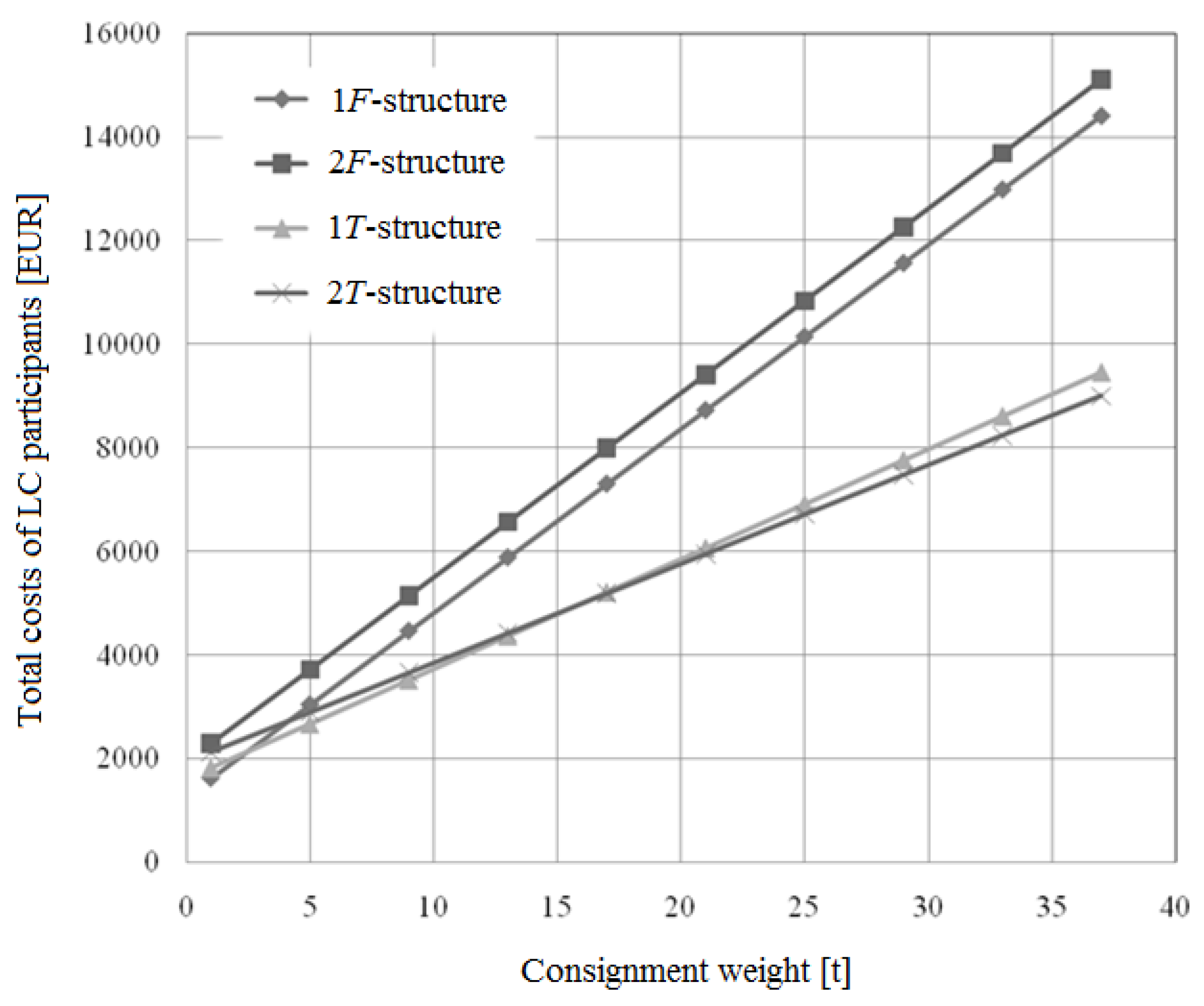
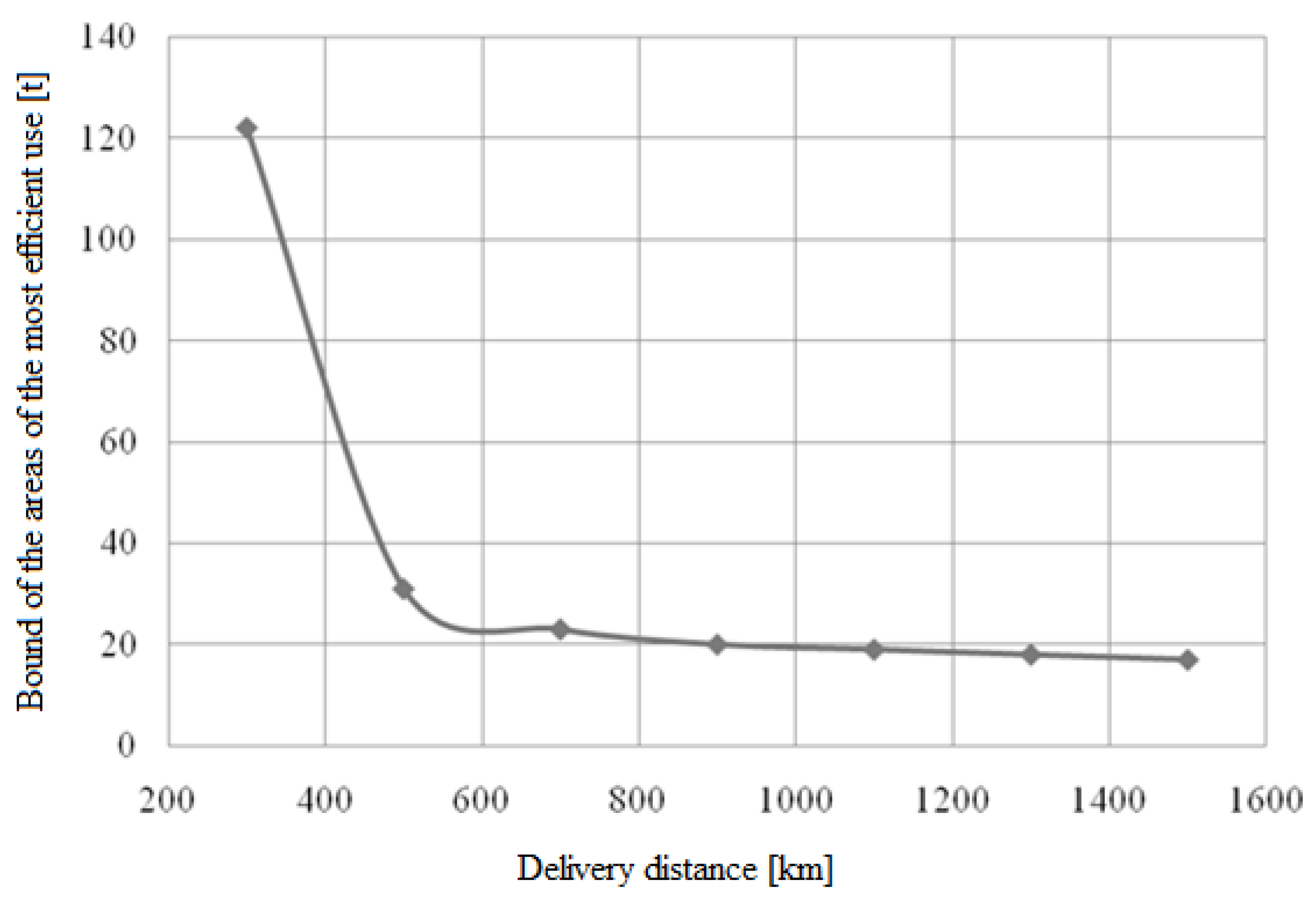
• the obtained solutions determine the bounds of the areas of the most efficient use of the alternative LC structures, the corresponding dependencies of the total costs form the lower polygonal chain on the graph.

For the pair of 1F- and 2F- structures, the boundaries of the area of the preferred use are determined as the roots of the following equation:

$$\begin{array}{l}\left(a_{Q2}^{1F}-a_{Q2}^{2F}\right)·Q^2+\left(a_{QL}^{1F}·L-a_{QL}^{2F}·L+a_Q^{1F}-a_Q^{2F}-a_{QL}^{C_A}·L^A-a_{QL}^{C_B}·L^B\right)·Q+\\ +\left(a_0^{1F}-a_0^{2F}+a_I^{1F}·I-a_I^{2F}·I+a_L^{1F}·L-a_L^{C_A}·L^A-a_L^{C_B}·L^B\right)=0.\end{array}$$

(24)

Similarly, the areas of preferred use are estimated for pairs of 1F and 1T variants, 1F- and 2T- variants, 2F- and 1T- variants, 2F- and 2T- variants, and 1T- and 2T- variants of LC that are based on the corresponding quadratic equations:

$$\begin{array}{l}\left(a_{Q2}^{1F}-a_{Q2}^{1T}\right)·Q^2+\left(a_{QL}^{1F}·L-a_{QL}^{1T}·L+a_Q^{1F}-a_Q^{1T}-a_{QL}^{C_A}·L^A-a_{QL}^{C_B}·L^B\right)·Q+\\ +\left(a_0^{1F}-a_0^{1T}+a_I^{1F}·I-a_I^{1T}·I+a_L^{1F}·L-a_L^{C_A}·L^A-a_L^{C_B}·L^B\right)=0;\end{array}$$

(25)

$$\begin{array}{l}\left(a_{Q2}^{1F}-a_{Q2}^{2T}\right)·Q^2+\left(\begin{array}{l}{a}_Q^{1F}-a_Q^{2T}+a_{QL}^{1F}·L-a_{QL}^{2T}·L-\\ -a_{QL}^{C_{A1}}·L^{A1}-a_{QL}^{C_{A2}}·L^{A2}-a_{QL}^B·L^B\end{array}\right)·Q+\\ +\left(a_0^{1F}-a_0^{2T}+a_I^{1F}·I-a_I^{2T}·I+a_L^{1F}·L-a_L^{C_{A1}}·L^{A1}-a_L^{A2}·L^{A2}-a_L^B·L^B\right)=0;\end{array}$$

(26)

$$\begin{array}{l}\left(a_{Q2}^{2F}-a_{Q2}^{1T}\right)·Q^2+\left(a_Q^{2F}-a_Q^{1T}+a_{QL}^{2F}·L-a_{QL}^{1T}·L\right)·Q+\\ +\left(a_0^{2F}-a_0^{1T}+a_I^{2F}·I-a_I^{1T}·I\right)=0;\end{array}$$

(27)

$$\begin{array}{l}\left(a_{Q2}^{2F}-a_{Q2}^{2T}\right)·Q^2+\left(\begin{array}{l}{a}_Q^{2F}-a_Q^{2T}+a_{QL}^{2F}·L-a_{QL}^{2T}·L+\\ +a_{QL}^{C_A}·L^A-a_{QL}^{C_{A1}}·L^{A1}-a_{QL}^{C_{A2}}·L^{A2}\end{array}\right)·Q+\\ +\left(a_0^{2F}-a_0^{2T}+a_I^{2F}·I-a_I^{2T}·I+a_L^{C_A}·L^A-a_L^{C_{A1}}·L^{A1}-a_L^{A2}·L^{A2}\right)=0;\end{array}$$

(28)

$$\begin{array}{l}\left(a_{Q2}^{1T}-a_{Q2}^{2T}\right)·Q^2+\left(\begin{array}{l}{a}_Q^{1T}-a_Q^{2T}+a_{QL}^{1T}·L-a_{QL}^{2T}·L+\\ +a_{QL}^{C_A}·L^A-a_{QL}^{C_{A1}}·L^{A1}-a_{QL}^{C_{A2}}·L^{A2}\end{array}\right)·Q+\\ +\left(a_0^{1T}-a_0^{2T}+a_I^{1T}·I-a_I^{2T}·I+a_L^{C_A}·L^A-a_L^{C_{A1}}·L^{A1}-a_L^{A2}·L^{A2}\right)=0.\end{array}$$

(29)

Since, according to Equations (16)–(19) $a_{Q2}^{1F}=a_{Q2}^{2F}=a_{Q2}^{1T}=a_{Q2}^{2T}=a_{Q2}^{FO}$, the factors for $Q^2$ in the Equations (24)–(29) are equal to 0. Thus, the presented quadratic equations degenerate to linear, which indicates the presence of, at most, one intersection point on the graphs of total costs corresponding to the considered LC structures. The boundaries $Q_{i-j}$ of preferred use areas for the i-th and j-th structures of the LC, in this case, are determined on the basis of the following expressions:

$$Q_{1F-2F}=\frac{a_0^{2F}-a_0^{1F}+a_I^{2F}·I-a_I^{1F}·I+a_L^{C_A}·L^A-a_L^{1F}·L+a_L^{C_B}·L^B}{a_Q^{1F}-a_Q^{2F}+a_{QL}^{1F}·L-a_{QL}^{2F}·L-a_{QL}^{C_A}·L^A-a_{QL}^{C_B}·L^B};$$

(30)

$$Q_{1F-1T}=\frac{a_0^{1T}-a_0^{1F}+a_I^{1T}·I-a_I^{1F}·I+a_L^{C_A}·L^A-a_L^{1F}·L+a_L^{C_B}·L^B}{a_Q^{1F}-a_Q^{1T}+a_{QL}^{1F}·L-a_{QL}^{1T}·L-a_{QL}^{C_A}·L^A-a_{QL}^{C_B}·L^B};$$

(31)

$$Q_{1F-2T}=\frac{a_0^{2T}-a_0^{1F}+a_I^{2T}·I-a_I^{1F}·I-a_L^{1F}·L+a_L^{C_{A1}}·L^{A1}+a_L^{A2}·L^{A2}+a_L^B·L^B}{a_Q^{1F}-a_Q^{2T}+a_{QL}^{1F}·L-a_{QL}^{2T}·L-a_{QL}^{C_{A1}}·L^{A1}-a_{QL}^{C_{A2}}·L^{A2}-a_{QL}^B·L^B};$$

(32)

$$Q_{2F-1T}=\frac{a_0^{1T}-a_0^{2F}+a_I^{1T}·I-a_I^{2F}·I}{a_Q^{2F}-a_Q^{1T}+a_{QL}^{2F}·L-a_{QL}^{1T}·L};$$

(33)

$$Q_{2F-2T}=\frac{a_0^{2T}-a_0^{2F}+a_I^{2T}·I-a_I^{2F}·I+a_L^{C_{A1}}·L^{A1}-a_L^{C_A}·L^A+a_L^{A2}·L^{A2}}{a_Q^{2F}-a_Q^{2T}+a_{QL}^{2F}·L-a_{QL}^{2T}·L+a_{QL}^{C_A}·L^A-a_{QL}^{C_{A1}}·L^{A1}-a_{QL}^{C_{A2}}·L^{A2}};$$

(34)

$$Q_{1T-2T}=\frac{a_0^{2T}-a_0^{1T}+a_I^{2T}·I-a_I^{1T}·I+a_L^{C_{A1}}·L^{A1}-a_L^{C_A}·L^A+a_L^{A2}·L^{A2}}{a_Q^{1T}-a_Q^{2T}+a_{QL}^{1T}·L-a_{QL}^{2T}·L+a_{QL}^{C_A}·L^A-a_{QL}^{C_{A1}}·L^{A1}-a_{QL}^{C_{A2}}·L^{A2}}.$$

(35)

The areas of the most efficient use of the LC structures, as shown in

Table 1. Areas of the most efficient use of LC structures for deliveries by road transport.

Delivery Distance	1F-Structure	2F-Structure	1T-Structure	2T-Structure
up to 300 km	up to 3 tons	-	3…122 tons	more than 122 tons
301…500 km	up to 3 tons	-	3…31 tons	more than 31 tons
501…700 km	up to 3 tons	-	3…23 tons	more than 23 tons
701…900 km	up to 2 tons	-	2…20 tons	more than 20 tons
901…1100 km	up to 2 tons	-	2…19 tons	more than 19 tons
1101…1300 km	up to 2 tons	-	2…18 tons	more than 18 tons
more than 1300 km	up to 2 tons	-	2…17 tons	more than 17 tons

, were obtained using the method described above based on Equations (30)–(35) for the expected value of the request interval equal to 2 h. The presented numeric results should be understood as an example describing the principle of justification of the best possible solution for the LC structure.

While analyzing the numerical results of the assessment of the areas of the most efficient use for considered ranges of demand parameters, the following implications must be mentioned:

• the use of the simplest version of the LC is optimal for the delivery by road transport of small consignments (up to three tons);
• the use in road transport of the LC variant with the participation of two freight forwarders is not characterized by the lowest possible total costs regardless of the values of the consignment weight and the delivery distance; therefore, the 2F-variant of the LC should only be used in cases when it is not possible to arrange delivery without the participation of the contractor forwarder; and,
• the bounds of the areas of the most effective LC structures (for the consignment volume as a parameter) inversely depend on the delivery distance.

Figure 7 shows the pattern of changes in the boundary of the areas of the most efficient use for 1T- and 2T-variants of the LC for the example considered in Table 1: the lesser the consignment weight, the bigger the delivery distance should be for 2T-structure to appear the better option in terms of the total costs.

The obtained dependency allows for us to conclude that the use of the LC with the participation of two freight terminals for short delivery distances is only advisable if the consignment weight is big enough (more than 100 tons). Additionally, vice versa—when the delivery distance is more than 500 km, the bound of the area of the most efficient use for the 2T-structure corresponds to a delivery weight of about 20 tons.

The proposed method for justification of the areas of the most efficient use for the considered variants of the LC structures has a significant practical value. The following managerial implications regarding the supply chain management procedures should be highlighted:

• having the areas substantiated for the given demand parameters, decision-makers (freight forwarders or other logistics operators) can choose the proper LC structure without calculating the costs for all possible alternative structures;
• the proposed methodology contributes to decreasing of the clients servicing time and reduces possible mistakes made by operators while making a decision concerning the LC structure, and in total – supports the sustainable operation of transport on a regional scale; and,
• the areas of the most efficient use of the LC structures can be implemented in specialized tools of information systems supporting decisions of logistics operators.

5. Conclusions

The selection of the optimal variant for the delivery of goods by road transport should be made on the basis of the minimum total costs of the LC participants—freight owners, carriers, freight forwarders, and freight terminals. The total costs of the LC participants are functionally determined by the structure of the chain, the parameters of the demand for transport services, and the parameters describing the impact on the LC of the external environment.

The structure of a LC for the delivery of goods by road transport can be assigned to one of the following options: 1F is the simplest structure with one forwarder, 2F is delivery with the participation of two forwarders without the involvement of freight terminals, 1T is delivery of a consignment through a freight terminal, and 2T is delivery with the involvement of two freight terminals. The combination of these variants of LC structures is a basic set of alternatives in the problem of justifying the optimal delivery variant.

The proposed methodology for evaluating the efficiency of the LC variants allows for considering the stochastic nature of the cargo delivery process by presenting the parameters of demand and technological indicators as random variables and takes into account the influence of the external environment on the LC effectiveness. It is necessary to simulate the technological processes of the shipment delivery to choose the best option for the LC structure to implement the described methodology. However, the proposed approach that is based on the evaluation of the areas of the most efficient use of the alternative LC structures allows for decision-makers to avoid simulation routines by choosing the best option for the given numeric characteristics of demand parameters.

Functional analysis of the demand parameters’ influence on the efficiency of the LC showed that, for any of the considered LC structures, the total costs quadratically depend on the consignment weight and linearly—on the delivery distance and the request interval. The results of the assessment of the areas of the most efficient use of various LC structures suggest that the use of the simplest LC variant is optimal for a one-time delivery of small consignments by road transport, and the 2F-variant should be used on road transport only in case it is not possible to arrange delivery without a partner forwarder.

As the directions of future research on the topic, the formation of the wider set of alternative LC structures and justification of the areas of their efficient use should be mentioned. The presented numeric results are case-sensitive and refer to freight deliveries by road transport between Ukraine and Poland, so additional experimental studies are needed to confirm obtained regularities.

References

1. Carvalho, H.; Fonseca, H. A multivariate data analysis of logistics structure as a factor of competitiveness. Braz. J. Oper. Prod. Manag. 2017, 14, 90–100. [Google Scholar] [CrossRef] [Green Version]
2. Melnyk, S.A.; Narasimhan, R.; DeCampos, H.A. Supply chain design: Issues, challenges, frameworks and solutions. Int. J. Prod. Res. 2014, 52, 1887–1896. [Google Scholar] [CrossRef] [Green Version]
3. Blos, M.F.; da Silva, R.M.; Wee, H.-M. A framework for designing supply chain disruptions management considering productive systems and carrier viewpoints. Int. J. Prod. Res. 2018, 56, 5045–5061. [Google Scholar] [CrossRef]
4. Yao, X.; Askin, R. Review of supply chain configuration and design decision-making for new product. Int. J. Prod. Res. 2019, 57, 2226–2246. [Google Scholar] [CrossRef]
5. Bányai, T.; Tamás, P.; Illés, B.; Stankevičiūtė, Ž.; Bányai, Á. Optimization of municipal waste collection routing: Impact of industry 4.0 technologies on environmental awareness and sustainability. Int. J. Environ. Res. Public Health 2019, 16, 634. [Google Scholar] [CrossRef] [PubMed] [Green Version]
6. Bányai, T. Real-time decision making in first mile and last mile logistics: How smart scheduling affects energy efficiency of hyperconnected supply chain solutions. Energies 2018, 11, 1833. [Google Scholar] [CrossRef] [Green Version]
7. Calleja, G.; Corominas, A.; Martínez-Costa, C.; de la Torre, R. Methodological approaches to supply chain design. Int. J. Prod. Res. 2018, 56, 4467–4489. [Google Scholar] [CrossRef]
8. Nobil, A.H.; Jalali, S.; Niaki, S.T.A. Financially embedded facility location decisions on designing a supply chain structure: A case study. Syst. Eng. 2018, 21, 520–533. [Google Scholar] [CrossRef]
9. Jahani, H.; Abbasi, B.; Alavifard, F.; Talluri, S. Supply chain network redesign with demand and price uncertainty. Int. J. Prod. Econ. 2018, 205, 287–312. [Google Scholar] [CrossRef]
10. Jabbarzadeh, A.; Fahimnia, B.; Sheu, J.-B.; Moghadam, H.S. Designing a supply chain resilient to major disruptions and supply/demand interruptions. Transp. Res. Part B Methodol. 2016, 94, 121–149. [Google Scholar] [CrossRef]
11. Claypool, E.G.; Norman, B.A.; Needy, K.L. Design for supply chain: An analysis of key risk factors. Ind. Eng. Manag. 2015, 4, 156. [Google Scholar] [CrossRef]
12. Samson, D.; Gloet, M. Integrating performance and risk aspects of supply chain design processes. Prod. Plan. Control 2018, 29, 1238–1257. [Google Scholar] [CrossRef]
13. Hoseinpour, P.; Ahmadi-Javid, A. Designing service system networks with interruption risks. Int. Trans. Oper. Res. 2019, 26, 2561–2578. [Google Scholar] [CrossRef]
14. Moreno-Camacho, C.A.; Montoya-Torres, J.R.; Jaegler, A.; Gondran, N. Sustainability metrics for real case applications of the supply chain network design problem: A systematic literature review. J. Clean. Prod. 2019, 231, 600–618. [Google Scholar] [CrossRef]
15. Yun, Y.S.; Chuluunsukh, A.; Gen, M. Design and implementation of sustainable supply chain model with various distribution channels. Adv. Intell. Syst. Comput. 2020, 1002, 469–482. [Google Scholar] [CrossRef]
16. Sherafati, M.; Bashiri, M.; Tavakkoli-Moghaddam, R.; Pishvaee, M.S. Supply chain network design considering sustainable development paradigm: A case study in cable industry. J. Clean. Prod. 2019, 234, 366–380. [Google Scholar] [CrossRef]
17. Allaoui, H.; Guo, Y.; Sarkis, J. Decision support for collaboration planning in sustainable supply chains. J. Clean. Prod. 2019, 229, 761–774. [Google Scholar] [CrossRef]
18. Razm, S.; Nickel, S.; Sahebi, H. A multi-objective mathematical model to redesign of global sustainable bioenergy supply network. Comput. Chem. Eng. 2019, 128, 1–20. [Google Scholar] [CrossRef]
19. Resat, H.G.; Unsal, B. A novel multi-objective optimization approach for sustainable supply chain: A case study in packaging industry. Sustain. Prod. Consum. 2019, 20, 29–39. [Google Scholar] [CrossRef]
20. Wang, F.; Lai, X.; Shi, N. A multi-objective optimization for green supply chain network design. Decis. Support Syst. 2011, 51, 262–269. [Google Scholar] [CrossRef]
21. Jabbarzadeh, A.; Haughton, M.; Pourmehdi, F. A robust optimization model for efficient and green supply chain planning with postponement strategy. Int. J. Prod. Econ. 2019, 214, 266–283. [Google Scholar] [CrossRef]
22. Almetova, Z.; Shepelev, V.; Shepelev, S. Optimization of Delivery Lot Volumes in Terminal Complexes. Transp. Res. Procedia 2017, 27, 396–403. [Google Scholar] [CrossRef]
23. Naumov, V. Modeling demand for freight forwarding services on the grounds of logistics portals data. Transp. Res. Procedia 2018, 30, 324–331. [Google Scholar] [CrossRef]
24. Rohaninejad, M.; Sahraeian, R.; Tavakkoli-Moghaddam, R. Multi-echelon supply chain design considering unreliable facilities with facility hardening possibility. Appl. Math. Model. 2018, 62, 321–337. [Google Scholar] [CrossRef]
25. Cui, J.; Zhao, M.; Li, X.; Parsafard, M.; An, S. Reliable design of an integrated supply chain with expedited shipments under disruption risks. Transp. Res. Part E Logist. Transp. Rev. 2016, 95, 143–163. [Google Scholar] [CrossRef] [Green Version]
26. Sajedinejad, A.; Chaharsooghi, S.K. Multi-criteria supplier selection decisions in supply chain networks: A multi-objective optimization approach. Ind. Eng. Manag. Syst. 2018, 17, 392–406. [Google Scholar] [CrossRef]
27. Sabri, Y.; Micheli, G.J.L.; Nuur, C. How do different supply chain configuration settings impact on performance trade-offs? Int. J. Logist. Syst. Manag. 2017, 26, 34–56. [Google Scholar] [CrossRef] [Green Version]
Figure 1. Model for choosing the optimal logistics chain (LC) structure.
Sustainability 12 01635 g001
Figure 2. The simplest variant of the LC structure.
Sustainability 12 01635 g002
Figure 3. The LC structure with two forwarders.
Sustainability 12 01635 g003
Figure 4. The LC structure with one terminal.
Sustainability 12 01635 g004
Figure 5. The LC structure with two terminals.
Sustainability 12 01635 g005
Figure 6. Dependency of the total costs of participants in the LC on the consignment weight.
Sustainability 12 01635 g006
Figure 7. Dependence of the boundary value of the areas of the most efficient use of 1T- and 2T- structures on the delivery distance.
Sustainability 12 01635 g007