Article

Prediction of Soil Nutrients Based on Topographic Factors and Remote Sensing Index in a Coal Mining Area, China

1
College of Resource and Environment, Shanxi Agricultural University, Shanxi 030801, China
2
National Experimental Teaching Demonstration Center for Agricultural Resources and Environment, Shanxi Agricultural University, Shanxi 030801, China
*
Author to whom correspondence should be addressed.
Sustainability 2020, 12(4), 1626; https://doi.org/10.3390/su12041626
Submission received: 15 January 2020 / Revised: 16 February 2020 / Accepted: 19 February 2020 / Published: 21 February 2020

Abstract

:
(1) Background: Coal mining operations caused severe land subsidence and altered the distributions of soil nutrients that influenced by multiple environmental factors at different scales. However, the prediction performances for soil nutrients based on their scale-specific relationships with influencing factors remains undefined in the coal mining area. The objective of this study was to establish prediction models of soil nutrients based on their scale-specific relationships with influencing factors in a coal mining area. (2) Methods: Soil samples were collected based on a 1 × 1 km regular grid, and contents of soil organic matter, soil available nitrogen, soil available phosphorus, and soil available potassium were measured. The scale components of soil nutrients and the influencing factors collected from remote sensing and topographic factors were decomposed by two-dimensional empirical mode decomposition (2D-EMD), and the predictions for soil nutrients were established using the methods of multiple linear stepwise regression or partial least squares regression based on original samples (MLSROri or PLSROri), partial least squares regression based on bi-dimensional intrinsic mode function (PLSRBIMF), and the combined method of 2D-EMD, PLSR, and MLSR (2D-EMDPM). (3) Results: The correlation types and correlation coefficients between soil nutrients and influencing factors were scale-dependent. The variances of soil nutrients at smaller scale were stochastic and non-significantly correlated with influencing factors, while their variances at the larger scales were stable. The prediction performances in the coal mining area were better than those in the non-coal mining area, and 2D-EMDPM had the most stable performance. (4) Conclusions: The scale-dependent predictions can be used for soil nutrients in the coal mining areas.

1. Introduction

Soil nutrients, including soil organic matter (SOM), soil available nitrogen (SAN), soil available phosphorus (SAP), and soil available potassium (SAK) are essential for plant growth, and thus, their spatial distribution is important for agricultural management. Traditionally, soil nutrient measurement is based on laboratory analysis of field soil samples, and the discrete sampling points may not provide continuous distributions of soil nutrients.
A number of methods, including geostatistical models [1], inverse distance weighted [2], trend surface analysis [3], and the like, resolve the spatial distribution of soil properties based on geospatial autocorrelation [4,5]. However, these methods are limited by sampling density, and the methods either fail to consider the environmental effects on soil nutrients or consider the environmental effects only at the sampling scale, causing their heterogeneous distribution at different scales with different intensities [6,7]. The qualitative and quantitative information of vegetation growth or land surface temperatures can be obtained from the electromagnetic radiation of remote sensing (RS), which indirectly demonstrates the distribution of soil nutrients [8,9,10,11]. Schillaci et. al. indicated that the application of an RS index could enhance the predicting performance of soil properties [12]. Meanwhile, topographic factors affect the transposition and redistribution of soil nutrient contents [13], and their effects on soil nutrients vary at different scales [14,15]. A number of prediction methods for soil properties based on their relationships with topographic factors are proposed [16], including the ensemble learning model [17], extended models [18], regression model [19], and so on. Nevertheless, these methods do not consider their multiscale relationships between soil nutrients and the covariates. Additionally, scale-specific correlations between soil properties and environmental factors are explored using the geostatistical approach [20], multivariate empirical mode decomposition [21,22], wavelet transform [14], and so on. However, these methods either failed to realize the prediction of soil properties or did not establish the validation model.
For the coal mining area, effects of human activities on the spatial distribution of soil nutrients should not be ignored, and their effects on the relationships between soil nutrients and environmental factors should also be considered [23]. Thus, the traditional methods are not suitable for describing the spatial distribution characteristics of soil nutrients in the coal mining areas. Therefore, the objective of this study was to establish the validation model of soil nutrients based on their multiscale relationships with RS index and topographic factors, and to assess the prediction accuracy of soil nutrients based on different methods in the coal mining and non-coal mining areas.

2. Materials and Methods

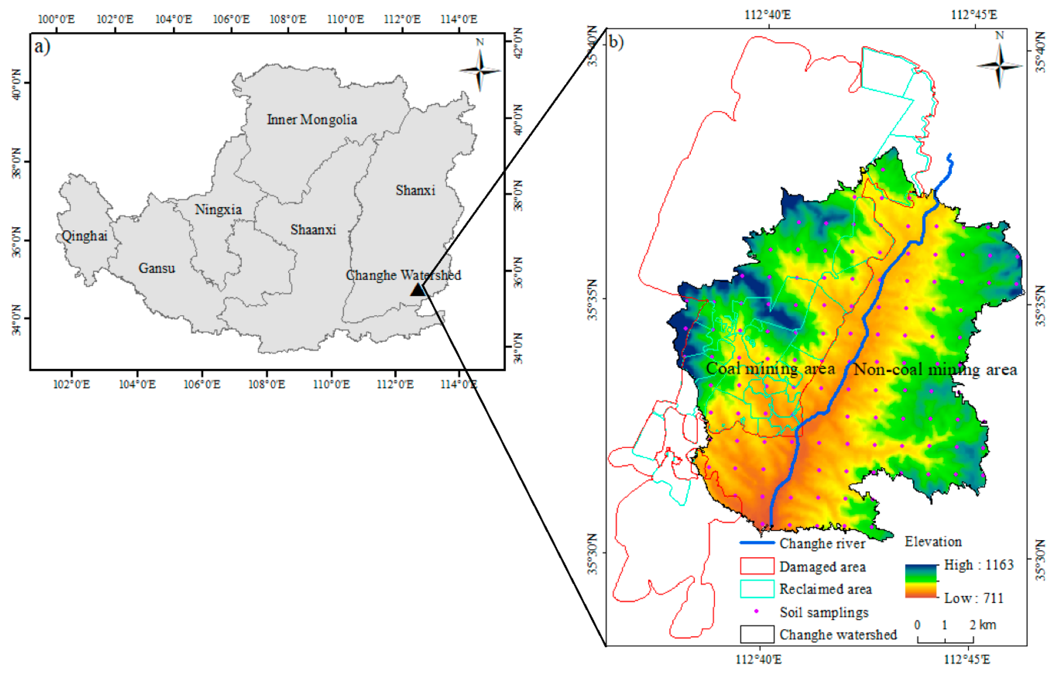
2.1. Study Area and Soil Sampling

The study area is the Changhe watershed located in the southeast of the Chinese Loess Plateau. It is bounded by latitude 35°30′14″–35°38′04″ N and longitude 112°27′39″–112°46′13″ E with a total area of about 116 km2 (Figure 1). The dominant soil type in the study area is calcaric cambisols [24], and the major crops in the arable land are maize, potato, and wheat. The Changhe river runs through the area from northeast to southwest and divides the study area into the eastern and western parts. In the western part, there are many coal mines containing hard coal. Most lands here were seriously damaged by coal mining activities, and some of them have been reclaimed. The range of elevation is from 718 to 1163 m in the coal mining area, while it is from 711 to 1040 m in the non-coal mining area, and the average elevations are 851 and 857 m for coal mining and non-coal mining areas, respectively.
A total of 120 sampling points was systematically established using the 1 × 1 km regular grid (Figure 1b), and soil samples were collected during 15–31 July 2015. At each point, three soil samples within a 5 m radius were collected using a soil auger and mixed together for one sample at a top layer of 0–20 cm according to the ploughing depth in the cultivated land of the study area. The samples were air-dried, gently crushed, and passed through a 2 mm sieve for soil nutrient determination. The SOM was measured by the dichromate oxidation method [25], SAN was determined by the diffusion method [26], SAP was obtained by the Olsen extraction method using alkaline sodium bicarbonate as the extractant in a 20:1 ratio [27], and SAK was extracted by a flame photometer [28]. Contents of sand (0.050–2.000 mm), silt (0.002–0.050 mm), and clay (<0.002 mm) were determined by the pipette method [29].

2.2. Collection of Environmental Factors

The products of moderate resolution imaging spectroradiometer (MODIS), including gross primary production (GPP, MOD17A2), net primary production (NPP, MOD17A3), land surface temperature for daytime and night (DLST and NLST, respectively, MOD11A2), evapotranspiration (ET, MOD16), and normalized difference vegetation index (NDVI, MOD13Q1) with 1 km resolution (the same with soil sampling scale of 1 km) in 2015 was downloaded (https://ladsweb.modaps.eosdis.nasa.gov/). The DLST, NLST, ET, and NDVI were used for extracting RS covariates in ENVI 5.3, including the intra-annual variance of the land surface temperature for daytime (DLSTV), the intra-annual variance of the land surface temperature for night (NLSTV), the annual mean evapotranspiration (ETM), the intra-annual standard deviation of evapotranspiration (ETD), the intra-annual variance of evapotranspiration (ETV), the annual mean NDVI (NDVIM), the inter-annual standard deviation of NDVI (NDVID), and the inter-annual variance of NDVI (NDVIV). The index of GPP, NPP, NDVIM, NDVID, and NDVIV indicated vegetation information and was selected because vegetation was the key source of the SOM. The index of DLSTV, NLSTV, ETM, ETD, and ETV indicated soil temperature and moisture and was selected because they were associated with the decomposition rates of SOM.
A digital elevation model (DEM) with 30 m spatial resolution (http://gdem.ersdac.jspacesystems.or.jp/) was downloaded. The DEM was used for extracting topographic factors, including elevation, aspect, slope, convergence index (CI), channel network base level (CNBL), flow accumulation (FA), LS factor (LS), topographic wetness index (TWI), valley depth (VD), and vertical distance to channel network (VDCN) in the software of SAGA ver. 6.4 (Department of Physical Geography, University of Göttingen, Germany) [30] and was resampled into the same resolution with an RS of 1 km in ArcGIS ver. 10.5 (ESRI Inc., Redlands, USA). The factors indicated topographic conditions, which were related to microclimate and soil erosion and thus affected the accumulation, decomposition, and flow of soil nutrients [12].

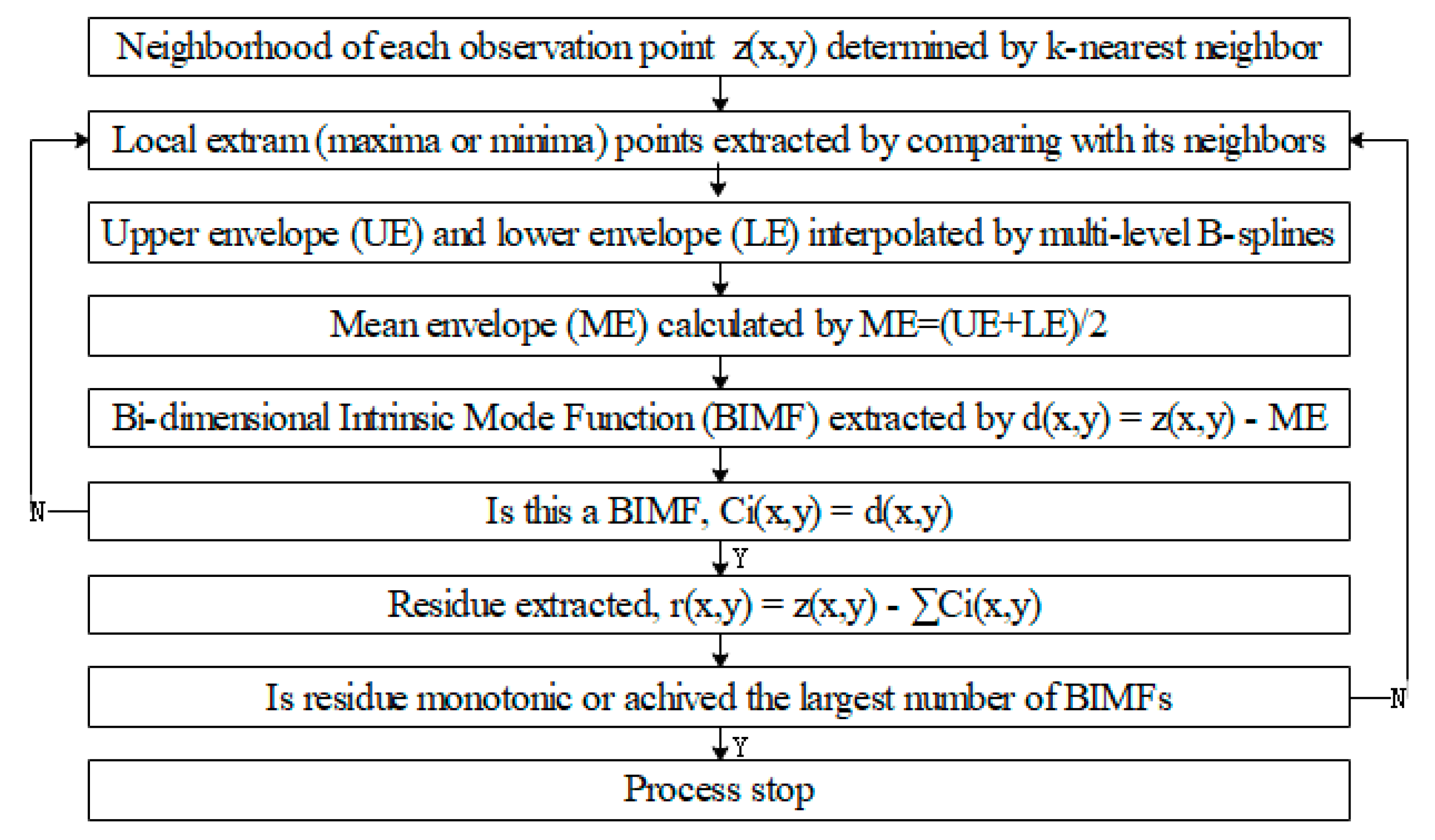
2.3. Two-Dimensional Empirical Mode Decomposition (2D-EMD)

Two-dimensional empirical mode decomposition has been used to separate the overall variation of any spatial or temporal dataset into different scale components called bi-dimensional intrinsic mode function (BIMFs) [31]. Unlike EMD finding the overall extrema, 2D-EMD determines the local extrema (maxima and minima) of the spatial dataset. The minima and maxima points of each location have to be interpolated, and the mean values of the interpolated minima and maxima points have to be calculated. The 2D-EMD for two-dimensional spatial dataset is defined as Equation (1).
z ( x , y ) = i = 1 N d i ( x , y ) + r ( x , y )
where z(x,y) was the original two dimensional spatial dataset, d i ( x , y ) is the BIMF, and r ( x , y ) is the residue. The main process of 2D-EMD can be seen in Figure 2. More detailed description of 2D-EMD can be found in other studies [32,33].

2.4. Data Analysis

Soil nutrients and the selected environmental factors were decomposed into three BIMFs and their corresponding residue in the “spemd” package in R ver. 3.6 (The University of Auckland, Oakland, New Zealand) [34] and guaranteed that each scale component contained at least 5% variance of the original data. However, the environmental factors of DLSTV, NLSTV, NDVIM, NDVID, and slope could be decomposed into only one BIMF and its residue, while the environmental factors of ETD and elevation were only decomposed into two BIMFs and its residue.
The percentage variance contributions of each BIMF and residue were obtained through the ratio of each BIMF variance to the variance of original data as Equation (2).
Variance   ( % ) =   V a r i a n c e   o f   e a c h   B I M F   ( o r   r e s i d u e ) v a r i a n c e   o f   o r i g i n a l   d a t a   a t   t h e   s a m p l i n g   s c a l e × 100
The Pearson’s correlation coefficients between soil nutrients and environmental factors at the sampling scale or the scale components (BIMFs and residue) were calculated.
The analysis of variance (ANOVA) was used to analyze soil nutrients between coal mining and non-coal mining areas. When the soil nutrients (SOM and SAN) had significant difference, different prediction models were established for the coal mining area and non-coal mining area, respectively. However, one prediction model was established for the entire area when soil nutrients had no significant difference. Regardless of one model or two different models for the coal mining and non-coal mining areas, 75% of sampling points were selected randomly as calibration samples, and 25% of sampling points were selected as validation samples. There were four different methods of prediction, including prediction from environmental factors at the sampling scale using multiple linear stepwise regression (MLSROri), from environmental factors at the sampling scale using partial least squares regression (PLSROri), from environmental factors at the scale component using PLSR (PLSRBIMF), and the combined method of 2D-EMD, PLSR, and MLSR (2D-EMDPM). For the method 2D-EMDPM, specifically, soil nutrients and the environmental factors were decomposed into BIMFs and residue using 2D-EMD; soil nutrients at each BIMF (or residue) were predicted from the environmental factors at the corresponding BIMF (or residue) using PLSR; soil nutrients at the sampling scale were estimated from the predicted soil nutrients at the BIMFs and residue using MLSR. The prediction performances were evaluated based on three parameters of coefficient of determination (R2), root mean square error (RMSE), and the ratio of performance to deviation (RPD). The R2, RMSE, and RPD are defined in Equations (3)–(5), respectively. The optimal number of latent variables (LV) for PLSR models were determined at the minimum value of root mean squared error of prediction (RMSEP) in the calibration model.
R 2 = 1 i = 1 n ( y i y ^ i ) 2 / i = 1 n ( y i y ¯ ) 2
R M S E = i = 1 n ( y i y ^ i ) 2 / n
R P D = S D / R M S E = n i = 1 n ( y i y ¯ ) 2 / i = 1 n ( y i y ^ i ) 2 / ( n 1 )
where n is the number of samples; y ¯ is the mean of the measured values; and y i and y ^ i are the measured and predicted values of soil nutrients in the ith sample, respectively.

3. Results

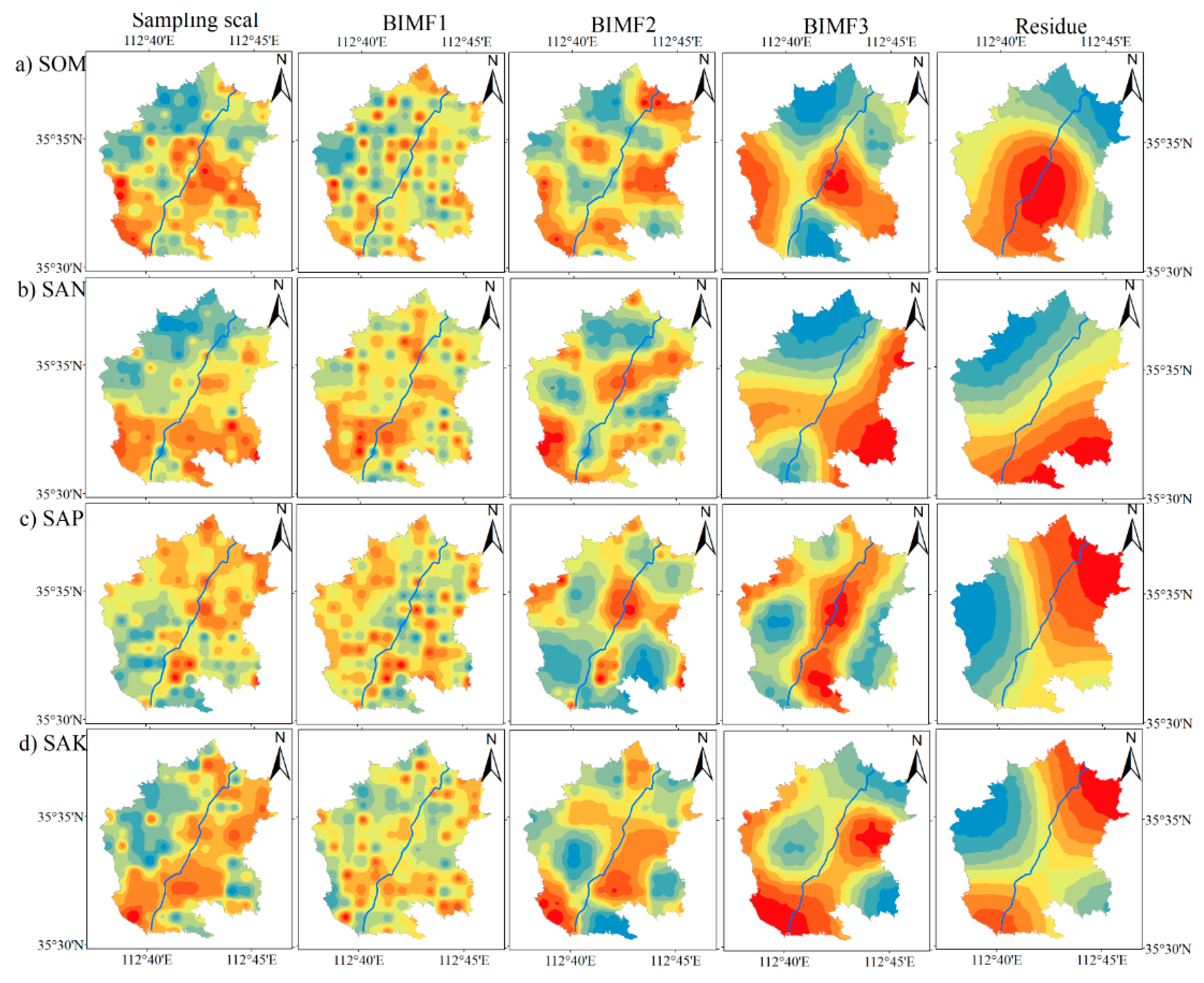
3.1. Soil Properties at the Sampling Scale

The basic statistics of soil nutrients and soil texture are shown in Table 1. The mean soil nutrients in the coal mining area were 17.42 g/kg, 32.44 mg/kg, 7.95 mg/kg, and 152.50 mg/kg for SOM, SAN, SAP, and SAK, respectively, which were lower than those in the non-coal mining area (19.88 g/kg, 39.40 mg/kg, 9.21 mg/kg, and 163.14 mg/kg for SOM, SAN, SAP, and SAK, respectively). The coefficients of variance (CVs) in the coal mining area were 44.73%, 37.12%, and 26.73% for SOM, SAN, and SAK, respectively, greater than those (28.09%, 30.26%, and 20.74% for SOM, SAN, and SAK, respectively) in the non-coal mining area. The greater CVs in the coal mining area might be attributed to mining practices in the area. The ANOVA analysis indicated that the spatial distribution of SOM and SAN between coal mining area and non-coal mining area were different. This data indicated that the predicting models for SOM and SAN should be established in the coal mining and non-coal mining areas separately, while the predicting models for SAP and SAK could be constructed in the coal mining and non-coal mining areas together. Obviously, the mean sand in coal mining area (0.23) was higher than that in the non-coal mining area (0.19); the mean silt in the coal mining area (0.48) was lower than that in the non-coal mining area (0.52); the mean clay in the coal mining and non-coal mining areas were similar. The spatial differentiation between coal mining area and non-coal mining area were significant for sand and silt, while it was non-significant for clay.
The relationships between soil nutrients and soil texture under the coal mining area, non-coal mining area, and the entire watershed are shown in Table 2. Despite the non-significant correlation between SOM and soil texture, SOM was positively related to silt in the coal mining area and positively correlated with clay in the non-coal mining area. Although silt had a non-significant relationship with SAN in the non-coal mining area, silt had a positive effect on SAN in the coal mining area and the entire area. The relationships between clay and SAP in the non-coal mining area and the entire area were significant. Notably, sand had significantly negative effects on SAK in the coal mining area, non-coal mining area, and the entire study area.

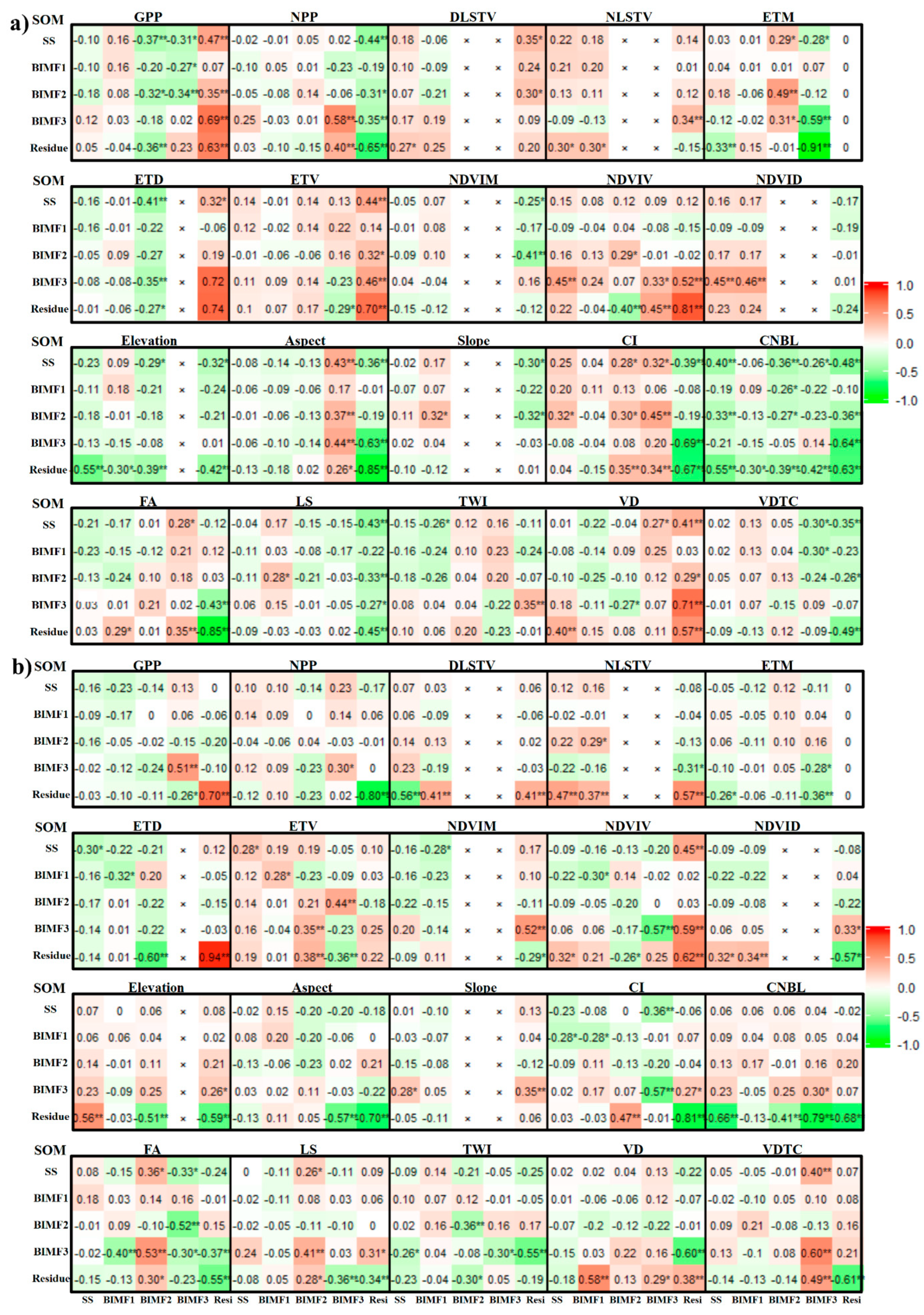
3.2. Scale-Specific Relationships of Soil Nutrients with Environmental Factors

The scale components for each soil nutrient were decomposed into three BIMFs and residue by 2D-EMD. The soil nutrients at the sampling scale and at these scale components are shown in Figure 3. The spatial distributions of SOM and SAN at the sampling scale were identical, while the spatial pattern of SAP and SAK at the residue were similar. Moreover, the distinction between coal mining and non-coal mining areas for SAN were obvious.
The percentages of variance explained by each scale component for soil nutrients are shown in Table 3. Obviously, the percentage of variance explained by BIMF1 were greater than half of the total variance, indicating the significantly stochastic effects on soil nutrients, such as coal mining operations. Notably, the percentages of variance explained by BIMF1 for SOM and SAN in the coal mining area were slightly lower than those in the non-coal mining areas, which might be attributed to the less cultivated activities because of the severe subsidence resulting from coal-mining operations. Thus, the effects of cultivated activities on soil nutrients were remarkable in the study area, especially for SAP. Conversely, the structured variance for SOM and SAN, which stand for the sum of BIMF2, BIMF3, and residue, were also greater in the coal mining area than those in the non-coal mining area.
The correlation coefficients between the scale component of SOM and the corresponding scale component of topographic factors or RS index are shown in Figure 4. In the coal mining area, GPP at BIMF2 and BIMF3 was negatively correlated with SOM at some scales, while GPP at residue was positively correlated with SOM at some scales. NPP at residue negatively correlated with SOM at some scales. The land surface temperatures for daytime and night (DLSTV and NLSTV) had less correlation with SOM at the residue. The factors of evapotranspiration (ETD and ETV) at residue had significantly positive relationship with SOM. The relationships between factors of NDVI and SOM indicated that NDVIV had greater effects on SOM, and the greatest coefficient was 0.81 at residue.
Elevation at all scales had a negative relationship with SOM at residue. Aspect at BIMF3 had a positive effect on SOM at almost all scales, while its residue had a negative effect on SOM at the sampling scale, BIMF3, and residue. The effects of slope on SOM distribution at different scales were not greater. CI at the sampling scale, BIMF2, and BIMF3 had positive effects on SOM at the sampling scale, BIMF2, and residue, while CI at the residue had negative effects on SOM at the sampling scale and at some scale components. The significant correlation between FA and SOM were identified at their residues. LS at residue negatively correlated with SOM, while the effects of TWI on SOM at most scales were not significant. VD at residue had a positive relationship with SOM at some scales, while VDCN at residue had a negatively correlation with SOM at some scales.
In the non-coal mining area, the correlation between influencing factors and SOM differed greatly at different scales, and they were slightly less than those in the coal mining area. Generally, the greatest correlation coefficients were identified at the residues of SOM and the influencing factors. The correlation coefficients between the scale component of SAN and the scale component of influencing factors are shown in Figure 5. The correlation coefficients of the influencing factors with SAN were generally greater than those with SOM. The relationships between GPP (NPP, DLSTV, ETD, ETV) at the residue and SAN at almost all scales were significant. The correlation between topographic factors at the residue and SAN at almost all scales were negatively significant except VD. Additionally, the correlations between influencing factors and SAN in the coal mining area were generally greater than those in the non-coal mining area.

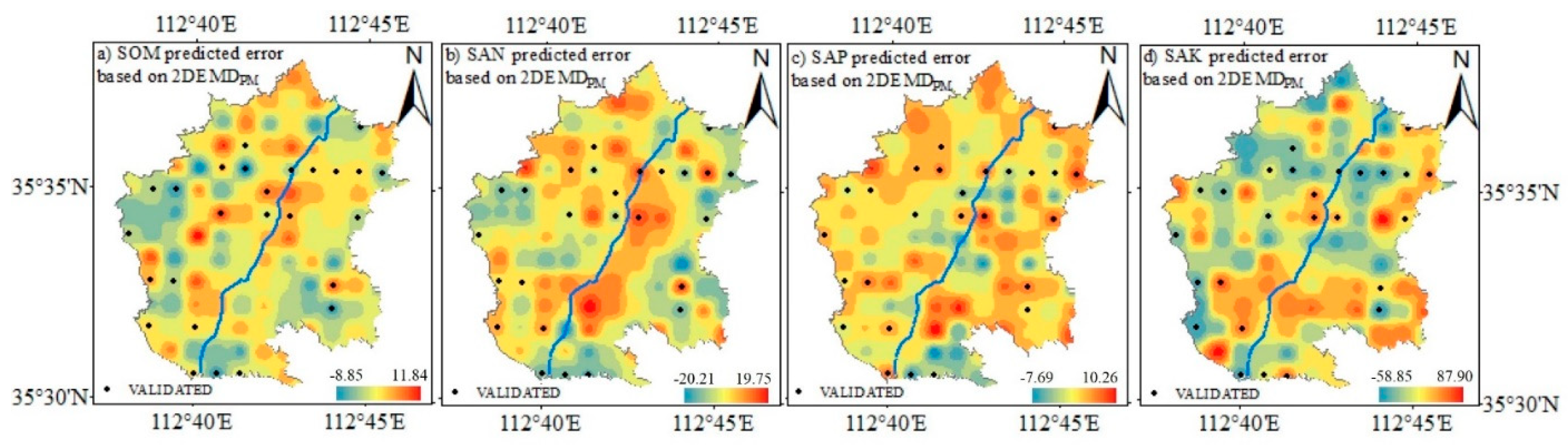
3.3. Soil Nutrient Prediction

The evaluating parameters for soil nutrient prediction are shown in Table 4. There were two methods (MLSROri and PLSROri) based on the soil nutrients and influencing factors at the sampling scales, and two methods (PLSRBIMF and 2D-EMDPM) based on the scale components of soil nutrients and influencing factors. Although the calibration accuracy of 2D-EMDPM was not the best among the four methods, its validation accuracy was the best, indicating that 2D-EMDPM was more stable than the other three methods.
The parameters for the developed 2D-EMDPM models for SOM, SAN, SAP, and SAK are shown in Table 5, and the numbers of latent variables (LVs) are listed. Generally, the LVs gradually increased with the increasing scales. Obviously, the predicting performance was the worst at the scale component of BIMF1, and they were becoming better at the larger scales. Meanwhile, the predicting accuracy for SOM and SAN was greater in the coal mining area than those in the non-coal mining area.
The spatial distributions of soil nutrient predicted errors based on 2D-EMDPM are shown in Figure 6. Considering the distinction between the coal mining area and non-coal mining area of SOM and SAN, different models were established. The greater predicted errors were distributed in a dispersed pattern and mainly located in the validated samples.
The measured SOM were generally lower than the predicted in the coal mining area, while the measured SOM were generally higher than the predicted in the non-coal mining area. This might be attributed to the mining operations resulting in the SOM leakage in the coal mining area, and the fertilizer application resulted in the higher content of SOM in the non-coal mining area. The predicted SAN were higher than the measured, which were mainly along the Changhe River in the non-coal mining area. The highly predicted SAP and SAK were also found in the non-coal mining areas, which might be attributed to the farming practices. However, the highly predicted SAP was also found in the coal mining area, which might be due to the great transformation easily affected by stochastic factors [35].

4. Discussion

Coal mining operations reduced the mean content of soil nutrients, which were consistent with previous studies [36,37], showing that land subsidence caused by coal mining could induce losses in surface soil nutrients. This might be due to the subsidence in the coal mining area resulting in the vertical leakage of soil nutrients from the top layer to the deeper layer [38]. Meanwhile, mining activities increased the variances of soil nutrients except SAP. In the Changhe Watershed, spatial distribution of SOM and SAN in the coal mining area and non-coal mining area were different, which were affected by the coal mining activities. However, the distributions of SAP and SAK were not altered by the coal mining activities, which might be attributed to the horizontal running off of soil nutrients decreasing the different patterns between the coal mining area and non-coal mining area.
The correlation coefficient between soil nutrients and the influencing factors varied greatly, and their correlation types were also different at the sampling scale and each scale component, similar to previous studies [39,40,41,42]. The correlations between soil nutrients and the influencing factors were generally non-significant at the scale component of BIMF1, which might be attributed to the stochastic effects (i.e., the effect of farming practices) resulting in the random distribution of SOM at the small scale of BIMF1. The spatial distributions of BIMF1 varied greatly (Figure 3), and the worst predicting performance at BIMF1 (Table 5) demonstrated the stochastic variation at the small scale of BIMF1. In addition, a previous study [31] also proved the stochastic variation of soil nutrients at the small scale of BIMF1. Consequently, predicting models that excluded BIMF1 could improve their stability of predicting performance. On the other hand, the total percentage of variance explained by BIMF2, BIMF3, and residue was even less than the percentage of variance explained by BIMF1, which revealed the lesser effect of the structured variance and the greater effect of stochastic variance affected by human activities. Therefore, the predicting performance based on the structured variance of soil nutrients would not be better even if excluded the stochastic variance (BIMF1) in the study area.
SOM predictions using PLSR based on the scale components were better than the other methods in the calibration model except SOM in the coal mining area, indicating that predicting methods based on the scale components could improve the predicting performance, in line with previous reports [14,21]. However, these studies only established the calibration model and did not validate the predicting accuracies. The 2D-EMDPM was chosen as the ideal method based on the validation accuracy, which indicated the stability of 2D-EMDPM. However, the prediction performance in the coal mining area was better than those in the non-coal mining area. This might be attributed to the lesser effect of cultivated activity on SOM and SAN in the coal mining area because of the severe coal mining subsidence. Meanwhile, the large variance in the coal mining area could also result in the better performance of soil nutrients prediction. Therefore, the effects of cultivated activities were stronger than the effects of mining operations on the spatial distribution of soil nutrients. The prediction models for SAP and SAK were not satisfied in the entire area, which might be due to the farming practices in the cultivated land, such as fertilizer applications.
Because the prediction accuracy was not significant at the stochastic variance of BIMF1, and the prediction accuracy was significant at the larger scales, the predictions at the sampling scale should exclude the stochastic variance of BIMF1. These data further indicated that the predicting method of 2D-EMDPM excluding BIMF1 was stable in the coal mining area and cultivated fields affected by human activities. Meanwhile, topographic factors and RS index were easily acquired from the internet, and soil samplings and measurement were not necessary. If 2D-EMDPM was stable in certain coal mining areas, this would facilitate the prediction of soil nutrients in the coal mining area. However, 2D-EMDPM was only applied for the validated dataset, which was randomly selected only once, and was not applied for all the possible datasets randomly selected. Meanwhile, 2D-EMDPM application in other coal mining areas was not included in this study, and further study is needed in the future for better predictions of soil nutrients.

5. Conclusions

(1) The mean soil nutrients were less, and their CVs were greater in the coal mining area than those in the non-coal mining area. Meanwhile, the correlation coefficients between soil nutrients and influencing factors were generally higher in the coal mining area than those in the non-coal mining area.
(2) The small scale of BIMF1 represented stochastic variance, and their relationships with soil nutrients were almost non-significant, which were influenced by human activities. The predictions for BIMF1 were also non-significant because of the unstable distributions.
(3) Although the predicting method of MLSRORI was sometimes best in the calibration models, its performance was particularly unstable in the validation model and should not be used in the areas affected significantly by coal mining operations or farming practices. The proposed method was 2D-EMDPM, which decomposed the soil nutrients and their covariates into four scale components, then predicted soil nutrients at each scale component from the corresponding scale of the covariates, and finally predicted soil nutrients at the sampling scale from the predicted soil nutrients at each scale except BIMF1. The method was stable in the calibration and validation models and should be validated in other coal mining areas in the world.

Author Contributions

H.Z. and R.B. conceived and designed the research. R.S. analyzed the data. Z.X. and C.L. discussed the results. H.Z. wrote the paper, while the other authors supported writing the paper. All authors have read and agreed to the published version of the manuscript.

Funding

This research was funded by the Natural Science foundation of Shanxi Province (201801D221103), the Research Project of Shanxi Scholarship Council of China (2017–075), and the Innovation Grant of Shanxi Agricultural University (2017ZZ07).

Acknowledgments

The authors would like to acknowledge to all reviewers who have given us valuable information.

Conflicts of Interest

The authors declare no conflict of interest.

References

  1. McBratney, A.B.; Mendonça Santos, L.M.; Minasny, B. On Digital Soil Mapping. Geoderma 2003, 117, 3–52. [Google Scholar] [CrossRef]
  2. Gong, G.; Mattevada, S.; O’Bryant, S.E. Comparison of the accuracy of kriging and IDW interpolations in estimating groundwater arsenic concentrations in Texas. Environ. Res. 2014, 130, 59–69. [Google Scholar] [CrossRef] [PubMed]
  3. Tang, X.; Xia, M.; Pérez-Cruzado, C.; Guan, F.; Fan, S. Spatial distribution of soil organic carbon stock in Moso bamboo forests in subtropical China. Sci. Rep. 2017, 7, 42640. [Google Scholar] [CrossRef] [PubMed] [Green Version]
  4. Zhang, Y.; Guo, L.; Chen, Y.; Shi, T.; Luo, M.; Ju, Q.; Zhang, H.; Wang, S. Prediction of Soil Organic Carbon based on Landsat 8 Monthly NDVI Data for the Jianghan Plain in Hubei Province, China. Remote Sens. 2019, 11, 1683. [Google Scholar] [CrossRef] [Green Version]
  5. Kumar, S.; Singh, R.P. Spatial distribution of soil nutrients in a watershed of Himalayan landscape using terrain attributes and geostatistical methods. Environ. Earth Sci. 2016, 75, 473. [Google Scholar] [CrossRef]
  6. Liu, Y.; Guo, L.; Jiang, Q.; Zhang, H.; Chen, Y. Comparing geospatial techniques to predict SOC stocks. Soil Tillage Res. 2015, 148, 46–58. [Google Scholar] [CrossRef]
  7. Malone, B.P.; Jha, S.K.; Minasny, B.; McBratney, A.B. Comparing regression-based digital soil mapping and multiple-point geostatistics for the spatial extrapolation of soil data. Geoderma 2016, 262, 243–253. [Google Scholar] [CrossRef]
  8. Angelopoulou, T.; Tziolas, N.; Balafoutis, A.; Zalidis, G.; Bochtis, D. Remote Sensing Techniques for Soil Organic Carbon Estimation: A Review. Remote Sens. 2019, 11, 676. [Google Scholar] [CrossRef] [Green Version]
  9. Nocita, M.; Stevens, A.; Wesemael, B.V.; Aitkenhead, M.; Bachmann, M.; Barthès, B.; Dor, E.B.; Brown, D.J.; Clairotte, M.; Csorba, A. Soil Spectroscopy: An Alternative to Wet Chemistry for Soil Monitoring; Advances in Agronomy; Elsevier: Cambridge, MA, USA, 2015; Volume 132, pp. 139–159. [Google Scholar]
  10. Zhu, H.; Xu, Z.; Jing, Y.; Bi, R.; Yang, W. Spatial variation and predictions of soil organic matter and total nitrogen based on VNIR reflectance in a basin of Chinese Loess Plateau. J. Soil Sci Plant Nutr. 2018, 18, 1126–1141. [Google Scholar] [CrossRef] [Green Version]
  11. Hu, W.; Chau, H.W.; Si, B.C. Vis-Near IR Spectroscopy for Soil Organic Carbon Content Measurement in the Canadian Prairies. CLEAN Soil Air Water 2015, 43, 1215–1223. [Google Scholar] [CrossRef]
  12. Schillaci, C.; Acutis, M.; Lombardo, L.; Lipani, A.; Fantappiè, M.; Märker, M.; Saia, S. Spatio-temporal topsoil organic carbon mapping of a semi-arid Mediterranean region: The role of land use, soil texture, topographic indices and the influence of remote sensing data to modelling. Sci. Total Environ. 2017, 601, 821–832. [Google Scholar] [CrossRef] [PubMed]
  13. Zhu, H.; Zhao, Y.; Nan, F.; Duan, Y.; Bi, R. Relative influence of soil chemistry and topography on soil available micronutrients by structural equation modeling. J. Soil Sci. Plant Nutr. 2016, 16, 1038–1051. [Google Scholar] [CrossRef] [Green Version]
  14. Zhu, H.; Wei, H.; Yaodong, J.; Yi, C.; Rutian, B.; Wude, Y. Soil organic carbon prediction based on scale-specific relationships with environmental factors by discrete wavelet transform. Geoderma 2018, 330, 9–18. [Google Scholar] [CrossRef]
  15. Hu, W.; Si, B.C. Soil water prediction based on its scale-specific control using multivariate empirical mode decomposition. Geoderma 2013, 193, 180–188. [Google Scholar] [CrossRef]
  16. Liu, E.; Liu, J.; Yu, K.; He, P.; Zhao, Z. Spatial Prediction of Forest Soil Organic Matter Based on Environmental Factors and R-STPS Interpolation Methods. Nongye Jixie Xuebao 2015, 46, 133–137. [Google Scholar] [CrossRef]
  17. Tajik, S.; Ayoubi, S.; Zeraatpisheh, M. Digital mapping of soil organic carbon using ensemble learning model in Mollisols of Hyrcanian forests, northern Iran. Geoderma Reg. 2020, 20, e00256–e00263. [Google Scholar] [CrossRef]
  18. Zhao, Z.; Yang, Q.; Sun, D.; Ding, X.; Meng, F.-R. Extended model prediction of high-resolution soil organic matter over a large area using limited number of field samples. Comput. Electron. Agric. 2020, 169, 105172. [Google Scholar] [CrossRef]
  19. Zhang, C.; Yang, Y. Can the spatial prediction of soil organic matter be improved by incorporating multiple regression confidence intervals as soft data into BME method? CATENA 2019, 178, 322–334. [Google Scholar] [CrossRef]
  20. Bourennane, H.; Salvador-Blanes, S.; Couturier, A.; Chartin, C.; Pasquier, C.; Hinschberger, F.; Macaire, J.-J.; Daroussin, J. Geostatistical approach for identifying scale-specific correlations between soil thickness and topographic attributes. Geomorphology 2014, 220, 58–67. [Google Scholar] [CrossRef]
  21. She, D.; Qian, C.; Timm, L.C.; Beskow, S.; Hu, W.; Leitzke Caldeira, T.; Montebello de Oliveira, L. Multi-scale correlations between soil hydraulic properties and associated factors along a Brazilian watershed transect. Geoderma 2017, 286, 15–24. [Google Scholar] [CrossRef]
  22. Zhu, H.; Cao, Y.; Jing, Y.; Liu, G.; Bi, R.; Yang, W. Multi-scale spatial relationships between soil total nitrogen and influencing factors in a basin landscape based on multivariate empirical mode decomposition. J. Arid Land 2019, 11, 385–399. [Google Scholar] [CrossRef] [Green Version]
  23. Xu, Z.; Zhang, Y.; Yang, J.; Liu, F.; Bi, R.; Zhu, H.; Lv, C.; Yu, J. Effect of Underground Coal Mining on the Regional Soil Organic Carbon Pool in Farmland in a Mining Subsidence Area. Sustainability 2019, 11, 4961. [Google Scholar] [CrossRef] [Green Version]
  24. Nachtergaele, F.; Van Velthuizen, H.; Verelst, L.; Batjes, N.; Dijkshoorn, K.; Van Engelen, V.; Fischer, G.; Jones, A.; Montanarella, L.; Petri, M. Harmonized World Soil Database; Food and Agriculture Organization of the United Nations: Rome, Italy, 2008. [Google Scholar]
  25. Nelson, D.W. Total Carbon, Organic Carbon and Organic Matter; ASA-SSSA: Madison, WI, USA, 1982; Volume 9, pp. 961–1010. [Google Scholar]
  26. Jackson, M.L. Soil Chemical Analysis: Advanced Course; UW-Madison Libraries Parallel Press: Madison, WI, USA, 2005. [Google Scholar]
  27. Olsen, S.R.; Cole, C.V.; Watanabe, F.S. Estimation of Available Phosphorus in Soils by Extraction with Sodium Bicarbonate; USDA: Washington, WA, USA, 1954. [Google Scholar]
  28. Isaac, E.; Kerber, J.D. Atomic Absorption and Flame Photometry: Techniques and Uses in Soil, Plant and Water Analysis; SSSA: Madison, WI, USA, 1972. [Google Scholar]
  29. Gee, G.W.; Bauder, J.W. Particle-size analysis. In Methods of Soil Analysis, Part 1. Physical and Mineralogical Methods, 2nd ed.; Klute, A., Ed.; The Agronomy Series; Elsevier: Madison, WI, USA, 1986; pp. 383–411. [Google Scholar]
  30. Schillaci, C.; Braun, A.; Kropáček, J. Terrain Analysis and Landform Recognition; British Society for Geomorphology: London, UK, 2015. [Google Scholar]
  31. Zhu, H.; Sun, R.; Bi, R.; Li, T.; Jing, Y.; Hu, W. Unraveling the local and structured variation of soil nutrients using two-dimensional empirical model decomposition in Fen River Watershed, China. Arch. Agron. Soil Sci. 2019, 1–14. [Google Scholar] [CrossRef]
  32. Huang, J.; Wu, C.; Minasny, B.; Roudier, P.; McBratney, A.B. Unravelling scale- and location-specific variations in soil properties using the 2-dimensional empirical mode decomposition. Geoderma 2017, 307, 139–149. [Google Scholar] [CrossRef]
  33. Xu, G.L.; Wang, X.T.; Xu, X.G. Improved bi-dimensional empirical mode decomposition based on 2D-assisted signals: Analysis and application. In IET Image Processing; Institution of Engineering and Technology: Stevenage, UK, 2011; Volume 5, pp. 205–221. [Google Scholar]
  34. Roudier, P. A Bi-Dimensional Implementation of the Empirical Mode Decomposition for Spatial Data. R Package Version 0.1-0. Available online: https://github.com/pierreroudier/spemd (accessed on 1 July 2018).
  35. Takeda, M.; Nakamoto, T.; Miyazawa, K. Phosphorus availability and soil biological activity in an Andosol under compost application and winter cover cropping. Appl. Soil Ecol. 2009, 42, 86–95. [Google Scholar] [CrossRef]
  36. Ma, K.; Zhang, Y.; Ruan, M.; Guo, J.; Chai, T. Land Subsidence in a Coal Mining Area Reduced Soil Fertility and Led to Soil Degradation in Arid and Semi-Arid Regions. IJERPH 2019, 16, 3929. [Google Scholar] [CrossRef] [Green Version]
  37. Sun, W.; Li, X.; Niu, B. Prediction of soil organic carbon in a coal mining area by Vis-NIR spectroscopy. PLoS ONE 2018, 13, e0196198. [Google Scholar] [CrossRef] [Green Version]
  38. Jing, Z.; Wang, J.; Zhu, Y.; Feng, Y. Effects of land subsidence resulted from coal mining on soil nutrient distributions in a loess area of China. J. Clean. Prod. 2018, 177, 350–361. [Google Scholar] [CrossRef]
  39. Hu, W.; Biswas, A.; Si, B. Application of multivariate empirical mode decomposition for revealing scale-and season-specific time stability of soil water storage. Catena 2014, 113, 377–385. [Google Scholar] [CrossRef]
  40. Zhou, Y.; Biswas, A.; Ma, Z.; Lu, Y.; Chen, Q.; Shi, Z. Revealing the scale-specific controls of soil organic matter at large scale in Northeast and North China Plain. Geoderma 2016, 271, 71–79. [Google Scholar] [CrossRef]
  41. Zhao, R.; Biswas, A.; Zhou, Y.; Zhou, Y.; Shi, Z.; Li, H. Identifying localized and scale-specific multivariate controls of soil organic matter variations using multiple wavelet coherence. Sci. Total Environ. 2018, 643, 548–558. [Google Scholar] [CrossRef] [PubMed]
  42. Si, B.C. Spatial scaling analyses of soil physical properties: A review of spectral and wavelet methods. Vadose Zone J. 2008, 7, 547–562. [Google Scholar] [CrossRef] [Green Version]
Figure 1. (a) Geographic location of the Changhe Watershed. (b) Distribution of sampling points.
Sustainability 12 01626 g001
Figure 2. Schematic presentation of the step of two-dimensional empirical mode decomposition (2D-EMD).
Sustainability 12 01626 g002
Figure 3. Spatial distributions of soil nutrients and their scale components of bi-dimensional intrinsic mode functions (BIMF1, BIMF2, BIMF3) and residue, including (a) soil organic matter (SOM), (b) soil available nitrogen (SAN), (c) soil available phosphorus (SAP), and (d) soil available potassium (SAK).
Sustainability 12 01626 g003
Figure 4. Correlation coefficients between soil organic matter (SOM) and topographic index or RS index at the sampling scale and their scale components of bi-dimensional intrinsic mode functions (BIMF1, BIMF2, BIMF3) and residue in (a) the coal mining and (b) the non-coal mining area. SS represents sampling scale, Resi represents residue.
Sustainability 12 01626 g004
Figure 5. Correlation coefficients between soil available nitrogen (SAN) and topographic index or RS index at the sampling scale and their scale components of bi-dimensional intrinsic mode functions (BIMF1, BIMF2, BIMF3) and residue in (a) the coal mining and (b) the non-coal mining area. SS represents sampling scale, Resi represents residue.
Sustainability 12 01626 g005
Figure 6. The spatial distributions of soil nutrients predicted errors based on 2D-EMDPM, including (a) soil organic matter (SOM) predicted error and (b) soil available nitrogen (SAN) predicted error with different models in the coal mining and non-coal mining areas; (c) soil available phosphorus (SAP) predicted error and (d) soil available potassium (SAK) predicted error with one prediction model in the entire area.
Sustainability 12 01626 g006
Table 1. Basic statistics of soil organic matter (SOM), soil available nitrogen (SAN), soil available phosphorus (SAP), and soil available potassium (SAK) and soil texture under coal mining and non-coal mining areas, respectively.
Soil NutrientsAreasMinMeanMaxStdCVANOVA
Fp-value
SOM
(g/kg)
Coal mining area1.1017.4236.427.7944.73a4.040.04
Non-coal mining area4.7219.8832.635.5828.09b
SAN
(mg/kg)
Coal mining area7.4232.4457.4812.0437.12a10.120.00
Non-coal mining area5.5639.4066.7511.9230.26b
SAP
(mg/kg)
Coal mining area0.957.9516.913.8348.15a2.600.11
Non-coal mining area1.529.2122.305.1155.48a
SAK
(mg/kg)
Coal mining area60.30152.50311.5540.7526.73a2.420.12
Non-coal mining area70.35163.14244.5533.8320.74a
Sand
(-)
Coal mining area0.090.230.640.0940.06a4.940.03
Non-coal mining area0.090.190.670.0947.93b
Silt
(-)
Coal mining area0.220.480.660.1021.37a6.130.01
Non-coal mining area0.180.520.700.1018.56b
Clay
(-)
Coal mining area0.140.290.480.0826.98a0.190.67
Non-coal mining area0.130.280.560.0827.25a
CV represents coefficient of variance. ANOVA represents analysis of variance, and different letters between coal mining area and non-coal mining area represent the significant difference of the soil nutrient at p < 0.05 level.
Table 2. The correlations between soil nutrients (SOM, SAN, SAP, and SAK) and soil texture under coal mining area, non-coal mining area, and the entire area, respectively.
Soil TextureCoal Mining AreaNon-Coal Mining AreaThe Entire Area
SOMSANSAPSAKSOMSANSAPSAKSOMSANSAPSAK
Sand −0.10−0.07−0.01−0.32 *0.010.08−0.06−0.44 **−0.09−0.05−0.07−0.39 **
Silt0.27 *0.34 **−0.120.32 *−0.23−0.10−0.150.160.100.18 *0.100.27 **
Clay−0.22−0.37 **0.20−0.070.29 *0.030.26 *0.32 *0.020.180.22 *0.09
SOM represents soil organic matter; SAN represents soil available nitrogen; SAP represents soil available phosphorus; SAK represents soil available potassium; * significant at p < 0.05; ** significant at p < 0.01.
Table 3. Percentage of variance explained by each bi-dimensional intrinsic mode functions (BIMF) or residue for soil nutrients (%).
Soil NutrientsAreaBIMF1BIMF2BIMF3ResidueSV
SOMCoal mining area53.5924.2419.476.8250.53
Non-coal mining area57.0819.9213.886.2440.04
SANCoal mining area55.5717.9912.157.1737.31
Non-coal mining area58.5915.119.0610.4234.59
SAPThe entire area73.6019.191.0511.4431.68
SAKThe entire area64.4820.244.805.6530.69
SOM: soil organic matter; SAN: soil available nitrogen; SAP: soil available phosphorus; SAK represents soil available potassium; SV: Structured variance, which equals BIMF2 + BIMF3 + Residue.
Table 4. Comparison of prediction parameters of soil nutrients for the methods of MLSROri, PLSROri, and PLSRBIMF and the combination of 2D-EMD, PLSR, and MLSR (2D-EMDPM).
Soil NutrientsMethodsCalibration AccuracyValidation Accuracy
R2RMSERPDR2RMSERPD
SOM in coal mining areaMLSROri0.66 **4.861.720.0829.200.21
PLSROri0.31 **6.851.220.28 *5.051.19
PLSRBIMF0.55 **5.591.500.20 *6.450.93
2D-EMDPM0.62 **5.081.640.64 **4.231.42
SOM in non-coal mining areaMLSROri0.52 **3.751.450.0259.500.10
PLSROri0.24 **4.681.160.125.820.98
PLSRBIMF0.18 **2.921.870.32 *5.301.08
2D-EMDPM0.48 **3.951.380.57 **4.111.39
SAN in coal mining areaMLSROri0.62 **7.421.660.0046.720.25
PLSROri0.49 **8.651.420.269.791.20
PLSRBIMF0.71 **6.511.890.45 **8.951.31
2D-EMDPM0.70 **6.681.840.61 **7.301.60
SAN in non-coal mining areaMLSROri0.71 **6.901.860.21164.810.06
PLSROri0.32 **10.451.230.30 *8.491.07
PLSRBIMF0.71 **6.871.870.19 *9.380.97
2D-EMDPM0.43 **9.521.340.40 **7.271.25
SAP in the entire areaMLSROri0.23 **4.221.150.0123.230.16
PLSROri0.10 **4.581.060.073.561.01
PLSRBIMF0.31 **4.001.210.14 *4.180.86
2D-EMDPM0.23 **4.221.150.15 *3.431.05
SAK in the entire areaMLSROri0.34 **31.401.230.00137.590.25
PLSROri0.26 **33.211.170.0140.060.86
PLSRBIMF0.46 **28.341.370.0638.330.90
2D-EMDPM0.34 **31.401.230.20 *33.021.05
MLSROri: multiple linear stepwise regression based on original samples; PLSROri: partial least squares regression based on original samples; PLSRBIMF: partial least squares regression based on bi-dimensional intrinsic mode function; 2D-EMDPM: the combined method of 2D-EMD, PLSR, and MLSR; SOM: soil organic matter; SAN: soil available nitrogen; SAP: soil available phosphorus; SAK: soil available potassium; * significant at p < 0.05; ** significant at p < 0.01.
Table 5. The properties of the developed 2D-EMDPM models for soil nutrients.
Soil NutrientsProcedureLVsCalibration AccuracyValidation Accuracy
R2RMSERPDR2RMSERPD
SOM in coal mining areaBIMF1 (PLSR)30.12 *5.651.050.135.451.09
BIMF2 (PLSR)220.95 **0.694.510.64 **2.021.35
BIMF3 (PLSR)230.99 **0.2110.690.87 **0.962.71
Residue (PLSR)411.00 **0.001496.611.00 **0.0618.04
SOM (MLSR)-0.62 **5.081.640.64 **4.231.42
−6.31 + 1.64 IMF2’ + 0.83 IMF3’ + 1.33 Residue’
SOM in non-coal mining areaBIMF1 (PLSR)20.114.290.980.163.760.80
BIMF2 (PLSR)150.81 **1.202.290.39 **2.451.16
BIMF3 (PLSR)381.00 **0.0547.470.78 **1.441.70
Residue (PLSR)351.00 **0.01175.190.99 **0.159.48
SOM (MLSR)-0.48 **3.951.380.57 **4.111.39
2.39 + 0.95 IMF2’ + 0.87 IMF3’ + 0.87 Residue’
SAN in coal mining areaBIMF1 (PLSR)10.09 *8.091.060.047.391.04
BIMF2 (PLSR)180.94 **4.021.100.65 **4.111.18
BIMF3 (PLSR)401.00 **0.01657.150.98 **0.5414.17
Residue (PLSR)421.00 **0.005327.920.99 **0.209.83
SAN (MLSR)-0.70 **6.681.840.61 **7.301.60
−3.09 + 0.44 IMF2’ + 1.36 IMF3’ + 2.69 Residue’
SAN in non-coal mining areaBIMF1 (PLSR)10.039.641.020.41 **7.530.86
BIMF2 (PLSR)200.87 **1.552.810.35 **5.030.87
BIMF3 (PLSR)401.00 **0.001024.420.92 **3.700.96
Residue (PLSR)411.00 **0.001742.531.00 **0.2713.76
SAN (MLSR)-0.43 **9.521.340.40 **7.271.25
−0.11 + 0.87 IMF2’ + 1.74 IMF3’ + 0.92 Residue’
SAP in the entire areaBIMF1 (PLSR)10.024.011.020.026.550.30
BIMF2 (PLSR)520.95 **0.454.400.50 **2.551.27
BIMF3 (PLSR)590.99 **0.0411.080.66 **0.281.60
Residue (PLSR)611.00 **0.01166.180.99 **0.1311.65
SAP (MLSR)-0.23 **4.221.150.15 *3.431.05
1.88 + 0.88 IMF2’ + 0.96 IMF3’ + 0.78 Residue’
SAK in the entire areaBIMF1 (PLSR)520.69 **17.391.800.01103.530.26
BIMF2 (PLSR)520.95 **3.664.610.56 **13.831.30
BIMF3 (PLSR)541.00 **0.3125.560.98 **1.326.92
Residue (PLSR)521.00 **0.1273.980.99 **0.7711.75
SAK (MLSR)-0.34 **31.401.230.20 *33.021.05
−27.27 + 0.96 IMF2’ + 0.60 IMF3’ + 1.16 Residue’
SOM: soil organic matter; SAN: soil available nitrogen; SAP: soil available phosphorus; SAK: soil available potassium; MLSR: multiple linear stepwise regression; PLSR: partial least squares regression; BIMF: bi-dimensional intrinsic mode functions; 2D-EMDPM: the combined method of 2D-EMD, PLSR, and MLSR; LVs: Number of latent variables; IMF2’, IMF3’, and Residue’ were the predicted IMF2, IMF3, and Residue by PLSR; * significant at p < 0.05; ** significant at p < 0.01.

