Spatio-Temporal Usage Patterns of Dockless Bike-Sharing Service Linking to a Metro Station: A Case Study in Shanghai, China

Abstract

The dockless bike-sharing (DLBS) system serves as a link between metro stations and travelers’ destinations (or originations). This paper aims to uncover spatio-temporal usage patterns of dockless bike-sharing service linking to metro stations for supporting scientific planning and management of the dockless bike-sharing system. A powerful visualization tool was used to analyze the differences in usage patterns in workdays and weekends. The travel distance distributions of using dockless bike-sharing near metro stations were investigated to shed light on the service area of the dockless bike-sharing system. Agglomerative hierarchical clustering was applied to analyze differences in usage patterns of metro stations located in different areas. The results show that the usage patterns of dockless bike-sharing on weekends are different from those on workdays. The average travel distance using the dockless bike-sharing system at weekends is significantly larger than that of workdays. The travel distance distribution could be nicely fitted by the Fréchet distribution of the Generalized Extreme Value (GEV) distribution family. The usage characteristics of shared bikes are correlated with land use and population density around metro stations. No matter in urban or suburban areas, there is a great demand for bike-sharing in densely populated areas with intensive land development, such as university towns in suburban areas. This study improves the understandings regarding the usage patterns of the DLBS system serving as a link between the final destinations (or originations) and metro stations. The results can be helpful to the operation and demand management of DLBS.

1. Introduction

Environment-friendly bike-sharing systems (BSSs) have rapidly developed and serve as an important contribution to solve first-and-last mile problems [1]. The dockless bike-sharing (DLBS) system is promoted by transportation managers and practitioners because of its advantages regarding little noise and air pollution [2] and improving the accessibility of public transportations [3,4,5]. In recent years, DLBS systems have been developed at a high rate of speed all over the world. As a type of free-flowing transportation shared bikes of DLBS systems can be an important part of the trip chain to make up for the shortcomings of public transport. There were 23,000,000 dockless bikes in the Chinese metropolis in late 2017 [6]. Over 1,700,000 dockless shared bikes were operated in Shanghai [7]. The explosion of dockless shared bikes has also created problems. Unreasonable resource allocation is one of them. Many cities that have shared bikes have such a problem. Some areas have a lot of available shared bikes lying idle, while some areas with high demand have a hard time seeing a shared bike. Some bike-sharing companies use manual dispatching to distribute shared bikes, but this is a very inefficient method. Shared bikes are also commonly used to resolve the last kilometer. Near the metro station, many people use shared bikes to get around, or even as a part of their commutes. Therefore, for the scientific planning and operation of the bike-sharing system, it is essential to investigate the spatio-temporal usage patterns of the dockless bike-sharing system and the usage patterns of dockless bike-sharing service linking to the metro station. In our study, Shanghai is taken as an example.

In this paper, two parts are contained to have a deep understanding of the usage patterns of DLBS in Shanghai. First, the characteristics of the usage frequency of shared bikes in time dimension are mined from the data set, and the characteristics of the usage distance between weekdays and weekends are explored. Second, a clustering algorithm is used to classify metro stations, and the shared bikes around these stations have different travel distance distributions of cycling, and land use characteristics around metro stations are used to interpret the classification results.

Many studies have been done on exploring the travelers’ usage patterns of bike-sharing systems. Li et al. [8] reported that the DLBS system has an adverse impact on the operation of the docked bike-sharing system because the DLBS system is more attractive and more convenient for people especially commuters in Nanjing, China. Pfrommer et al. [9] adopted historical data of a bike-sharing system to explore the patterns of bike-sharing mobility in London. They found that weekday usage had two peaks, while weekend usage just had one peak in the middle of the day. Deng et al. [10] indicated that the usage of shared bikes in workday showed two obvious rush hours in Beijing, China. Du et al. [11] constructed a model framework for discovering the usage patterns of the free-floating bike-sharing system. There were two peaks of travel time and distance of shared bike using in Yangpu and Hongkou District in Shanghai. Tao et al. [12] analyzed the spatio-temporal usage characteristics of the traditional public bike-sharing system in Nanning, a medium-sized city in China. Different from large cities, the peak of usage can be found later on weekdays, and people prefer to use a bike on weekend evenings in Nanning. The usage patterns of bike-sharing systems in different cities are various because each city has its special features of city scale, city layout, people’s working, and living styles.

Several studies have explored the general travel distance using the bike-sharing system. Du et al. [9] adopted three distributions (Power Law, Exponential, Lognormal) to explore usage patterns of bike-sharing systems and found that lognormal distribution performed best. Based on trip data from eight cities, Kou et al. [13] applied five different probability distributions (Power Law, Exponential, Lognormal, Gamma, and Weibull) to fit the travel distance distributions of bike-sharing. They found that the travel distance and duration distribution of bike-sharing systems with different scales obey different distribution rules. The travel distance and duration follow a lognormal distribution in larger bike-sharing systems, while the distribution for smaller systems varies among Weibull, gamma, and lognormal. Cities of different sizes have different traffic composition and land use characteristics, which lead to different cycling distance requirements. Du et al. [11] and Lv et al. [14] analyzed the travel distance rule of bike-sharing in Shanghai in general and without time distinction. The distance people ride varies from workdays to weekends. Ma et al. [15] revealed that the average activity distance of metro-bike-sharing on weekends was smaller than that on weekdays in Nanjing, China. Moreover, the distance of using bicycles in different areas of the same city should be different, such as the city center and suburbs, because the land use characteristics and population density of different areas of the city are different.

The usage characteristics of DLBS systems around metro stations and in different areas in a city are very necessary for the distribution of shared bikes by operators, so some studies have been done to understand it. Land use characteristics in different areas can have an influence on using shared bikes. Based on bike-sharing data within a specified distance of a metro station, Li et al. [16] used K-means clustering to analyze usage patterns of DLBS systems for metro stations in Nanjing City, China. The results showed that metro stations were clustered into five types on weekdays and three types on weekends, respectively. There was a strong correlation between the surrounding environment and the distribution of clusters. Deng et al. [8] found that the cycling effected by the spatial elements such as public traffic, trade, and dining, showed different spatial characteristics. Cycling areas were divided into five categories: tide-type, single-way type, incompact connection type, distance allowing type, and short connection type. Zhang et al. [17] demonstrated that the usage frequency of shared bikes decreased from metro stations to the outlying areas by visualizing cycling in Shanghai. The farther away from the subway station, the lower the population density and the lower the demand for bicycles. Zhao et al. [18] found that the travel distance was the most vital factor influencing the usage rate of cycling between home or workplace and metro station. Ma et al. [15] constructed a spatial error model and an ordinary least squares regression to explore the effects of the exterior environment of the metro stations and revealed that the closer it is to the central business district (CBD), the smaller space there is for metro-bike-sharing activity. The development of the city center is intensive, with dense buildings and rich transportation modes, such as buses and taxis. Based on the GPS data of DLBS systems in Singapore, Shen et al. [19] used spatial autoregressive models to mine Spatio-temporal patterns of bike utilization. The result showed that high land-use mixtures and convenient public transportation had positive impacts on the usage of dockless bikes, while bad weather conditions had negative influences. Zhang et al. [20] applied OD matrix analysis and hierarchical clustering to explore the general usage characteristics of BSS in Zhongshan, China. In the center of the city, the demand for bikes is relatively high because of the high degree of land development and high population density and activity frequency.

This paper stands in the wake of existing studies to investigate the usage patterns of bike-sharing and the DLBS linking to metro stations. This study not only explores the usage dynamic characteristics of the DLBS system but also mainly uses the travel distance distribution of shared bikes near metro stations to explore the usage characteristics of the DLBS system. Firstly, a powerful visualization tool is used to explore the dynamic usage characteristics of DLBS systems based on passive GPS data of the bike-sharing system. The distributions of travel distance using the bike-sharing system on weekends and workdays are fitted by lognormal distribution and generalized extreme value distribution to explore travel distance distribution rule and potential differences. Secondly, an agglomerative hierarchical clustering algorithm is used to classify the metro stations with different distributions of travel distance, the usage characteristics of shared bikes near different metro stations can be further understood. The agglomerative hierarchical clustering can get the real clustering results which match the actual situation. Through the land-use features gained from the Amap website (https://lbs.amap.com/api/javascript-api/example/map/map-english/), we explore the influences of land use on the usage pattern of DLBS linking to metro stations. The results of this study will not only enhance the understandings concerning the operating state and usage patterns of DLBS systems, which can support the reasonable planning and dispatching of DLBS systems but also for doing urban planning. For example, companies are encouraged to adopt time-sharing systems to reduce the intensity of morning and evening peaks in cities. Improving the public transportation system near subway stations with long cycling distances is conducive to improving people’s commuting efficiency.

2. Methodology

2.1. Data Source

The data used in this study is the DLBS usage data in Shanghai. The data of dockless shared bikes were extracted from open-source websites. Bike ID, Time, Lock status, Longitude, and Latitude were included in the dataset. The data from 26 August 2018 to 1 September 2018 (from Sunday to Saturday) were used in this study. There are 24,601,009 pieces of data. Data related to metro stations of Metro Line 9 were extracted before analyzing the usage patterns of DBLS linking to metro stations. There are 35 stations on Metro Line 9. Names and IDs of each station are displayed in

Table 1. Names and IDs of stations on Metro Line 9.

ID	Name	ID	Name	ID	Name
1	Caolu	13	Xiaonanmen	25	Qibao
2	Minlei Ro.	14	Lujiabang Ro.	26	Zhongchun Ro.
3	Gutang Ro.	15	Madang Ro.	27	Jiuting
4	Jinhai Ro.	16	Dapuqiao	28	Sijing
5	Jinji Ro.	17	Jiashan Ro.	29	Sheshan
6	Jinqiao	18	Zhaojiabang Ro.	30	Dongjing
7	Tai’erzhuang Ro.	19	Xujiahui	31	Songjiang University Town
8	Lantian Ro.	20	Yishan Ro.	32	Songjiang Xincheng
9	Fangdian Ro.	21	Guilin Ro.	33	Songjiang Sports Center
10	Middle Yanggao Ro.	22	Caohejing Hi-Tech Park	34	Zuibaichi Park
11	Century Avenue	23	Hechuan Ro.	35	Songjiang South Railway Statioon
12	Shangcheng Ro.	24	Xingzhong Ro.

and marked in Figure 1. After reformatting the original data, the complete travel information of the usage of the shared bike includes bike id, start time, start longitude, start latitude, return time, return longitude, return latitude, and service time. A final data structure sample is shown in

Table 2. Final structure of the data.

Bike ID	Start Time	Start Longitude	Start Latitude	Return Time	Return Longitude	Return Latitude	Service Time/s
169·B4	2018/08/26 07:45:01	121.398772532346	31.2595986596458	2018/08/26 07:57:48	121.386097072529	31.2508800507453	767

.

Firstly, we mined the daily usage patterns of DLBS in a week. The lognormal distribution and Generalized Extreme Value (GEV) distribution were applied to fit the travel distance for the bike using in workdays and weekends, respectively. Secondly, the agglomerative hierarchical clustering algorithm was applied to explore usage patterns of DLBS near stations in different areas. After clustering, the distributions of travel distance in different clustering were fitted. The available data merely provide the travel time of using DLBS. According to the results of recent research [14], the average cycling speed is 8.6 km/h in Shanghai. Therefore, we refer to the speed of 8.6 km/h to transform the travel time to travel distance of each cycling trip.

2.2. A Visualization Tool

To explore a week of the usage characteristics of DLBS systems, Seaborn was adopted to visualize and analyze the usage of DLBS systems. Seaborn is a library for making statistical graphics in Python. It is built on top of Matplotlib and closely integrated with Pandas data structures.

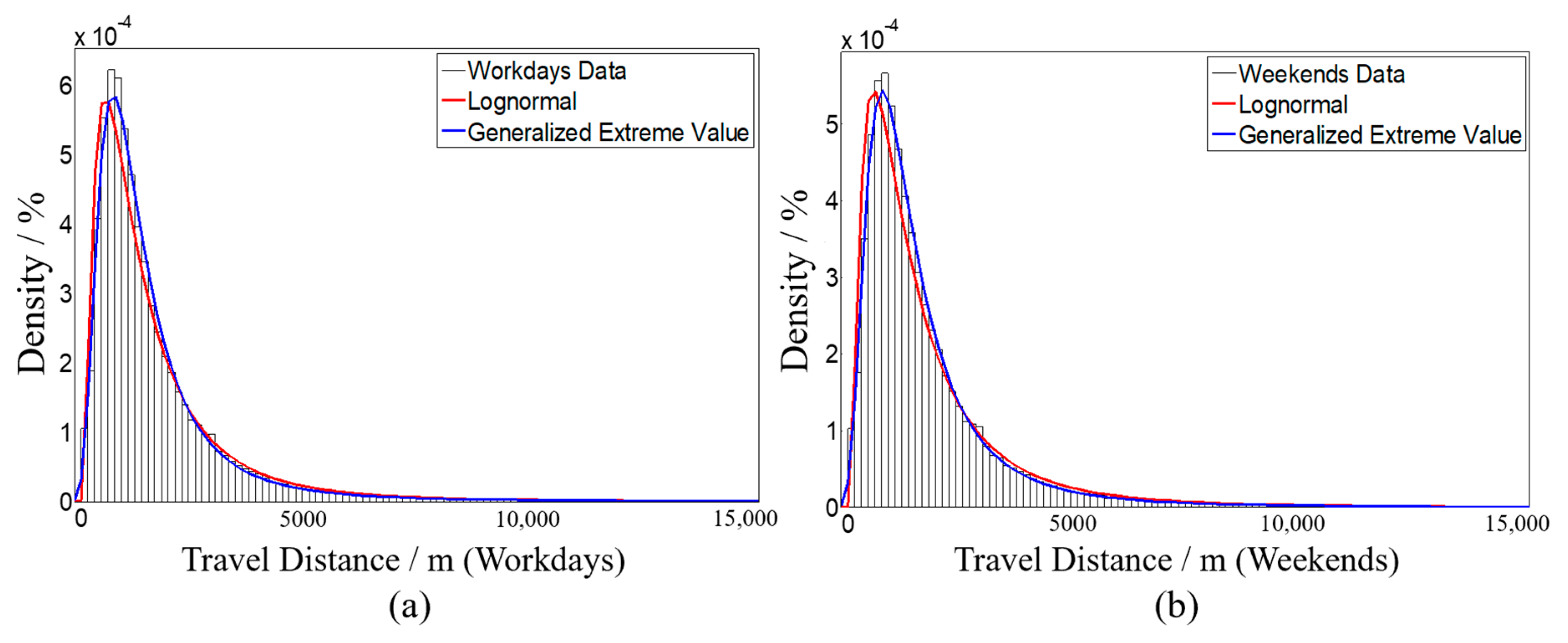
2.3. Probability Modeling

For deeply exploring the distribution of travel distance of DLBS systems, it is essential to construct the probability distribution models to fit cycling distance. The lognormal distribution and GEV distribution were applied in this study. The Gumbel, Fréchet, and Weibull distributions are united as GEV distribution, which allows a continuous range of possible shapes. These three distributions are also known as type I, II and III extreme value distributions. The GEV distribution is parameterized with three parameters, shape parameter, location parameter, and scale parameter. Equation (1) is the probability density function of the GEV distribution.

$$f(x;\mu ,\sigma ,\xi )=\frac{1}{\sigma }{\left[1+\xi (\frac{x-\mu }{\sigma })\right]}^{-1/\xi -1}\exp \left\{{\left[1+\xi (\frac{x-\mu }{\sigma })\right]}^{-1/\xi }\right\},$$

(1)

where $\xi$, $\mu$, and $\sigma$ represent the shape, location, and scale of the distribution function, respectively. The scale parameter $\sigma$ and 1 + $\xi \left(x-\mu \right)$ must greater than 0. The shape and location parameter can take on any real value. The tail of the distribution is governed by the shape parameter $\xi$. The sub-families defined by $\xi$ = 0, $\xi$ > 0 and $\xi$ < 0 are the Gumbel, Fréchet, and Weibull families, respectively.

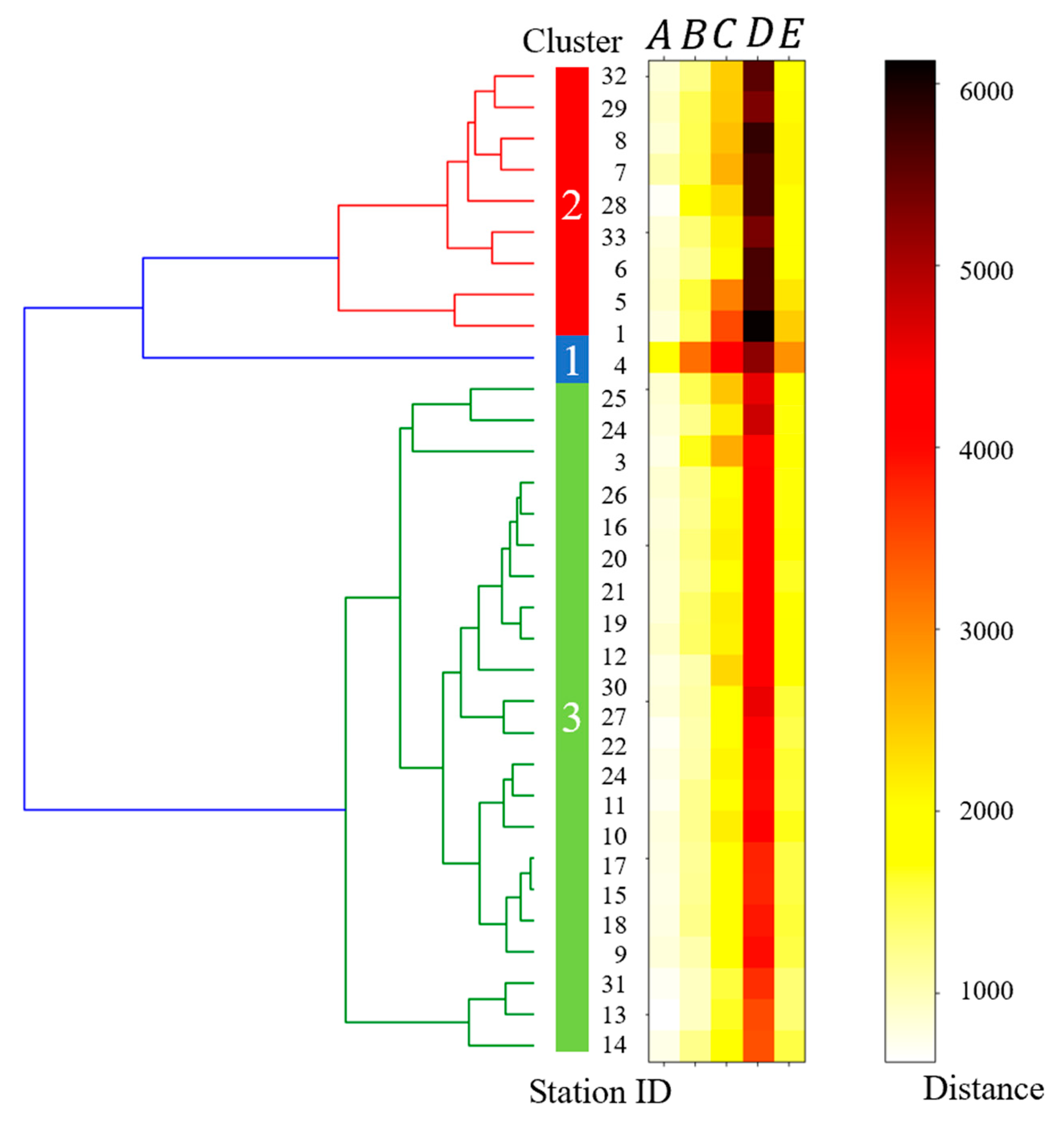
2.4. Agglomerative Hierarchical Clustering

In order to explore the different usage patterns of DBLS related to metro stations in different areas and investigate the influences of land use characteristics on the usage patterns of DLBS, agglomerative hierarchical clustering algorithm, one of the hierarchical clustering methods was applied to group the metro stations into different categories. The agglomerative hierarchical clustering algorithm is featured by the method of bottom-up and can be featured by greedy. The flow of agglomerative hierarchical clustering algorithm is shown in Algorithm 1. Each metro station has its distribution of travel distance of cycling. The dataset including the 25, 50, 75, and 90 percentile and the mean value of travel distance is used as features of the usage pattern of DLBS near different metro stations. Similar travel distance distribution can be grouped into a cluster by agglomerative hierarchical clustering.

The dynamic tree cutting method can be used to search for the best clustering result based on the dendrogram. In fact, actual demand is the determinant of clustering results. We can cut the clustering tree at a height close to the root to obtain a rough clustering result. Cluster trees can be cut at higher levels to generate more clusters for more refined clustering results.

A distance matrix is the input of the algorithm as shown in Equation (2).

$$D=\left[\begin{array}{ccc}{d}_{11}& \dots & d_{1n}\\ ⋮& d_{ij}& ⋮\\ d_{n1}& \dots & d_{nn}\end{array}\right],$$

(2)

where $n$ is the total number of metro stations; $d_{ij}$ is the squared Euclidean distance of two feature vectors as shown in Equation (3).

$$d_{ij}=d({\mathsf{\omega }}^i,{\mathsf{\omega }}^j)=\Vert {\mathsf{\omega }}^i-{\mathsf{\omega }}^j{\Vert }_2^2.$$

(3)

Equation (4) is the feature vector of every station.

$${\mathsf{\omega }}^m=({\omega }_A^m,{\omega }_B^m,{\omega }_C^m,{\omega }_D^m,{\omega }_E^m),m\in M,$$

(4)

where M is the set of metro stations and A, B, C, D, E represent 25, 50, 75, 90 percentile and mean value of travel distance distribution of station $m$, respectively.

Hierarchical clustering is the basic procedure in this algorithm. Complete linkage was used as the linkage criteria in our study, which means that the distance between the sample pairs of every two clusters is the largest.

$$\max \{d({\mathsf{\omega }}^i,{\mathsf{\omega }}^j):i,j\in K\},$$

(5)

where, K is the set of clusters.

Algorithm 1 Agglomerative Hierarchical Clustering Algorithm

Input: the original dataset $X=\{{\mathbf{x}}_1,{\mathbf{x}}_2,\cdots ,{\mathbf{x}}_n\}$; cluster distance measurement function $d_{\max }$; number of clusters $k$. Output: Cluster partition results. $C=\{C_1,C_2,\cdots ,C_k\}$ Process: for j = 1, 2, …, n do  $C_j=\left\{{\mathbf{x}}_j\right\}$ end for for i = 1, 2, …, n do  for j = i+1, 2, …, n do   $D(i,j)=d(C_i,C_j)$;   $D(j,i)=D(i,j)$  end for end for Sets the number of current clusters: $q=n$. while $q>k$ do  Find the two closest clusters $C_{i*}$ and $C_{*j}$;  Combine $C_{i*}$ and $C_{*j}$: $C_{i*}=C_{i*}\cup C_{*j}$;  for $j=j*+1,j*+2,\dots ,q$ do   Renumber cluster $C_j$ to $C_{j-1}$  end for  Delete row $j*$ and column $j*$ of the distance matrix $D$;  for $j=j*+1,j*+2,\dots ,q-1$ do   $D(i*,j)=d(C_{i*},C_j)$;   $D(j,i*)=D(i*,j)$  end for  $q=q-1$ end while

3. Results and Discussion

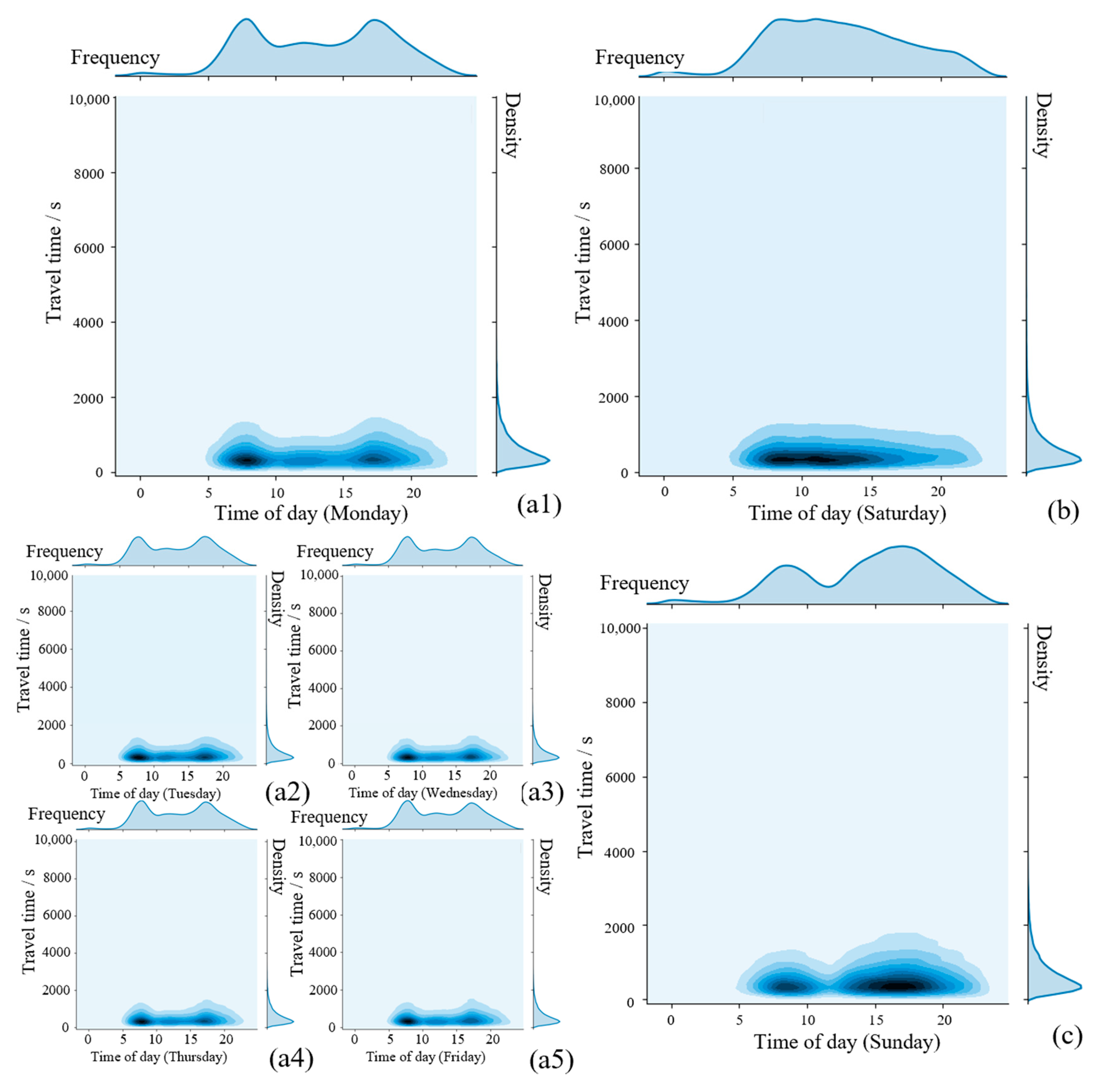
3.1. Usage Patterns of DLBS in Different Days of a Week

The usage patterns of DLBS in a week are shown in Figure 2. The kernel density map shows the travel time density of each cycling at different times. The number of shared bike usage is shown at the top of each figure. The whole travel time density of shared bikes is shown on the right side of each figure. The subfigures (a1–a5) present Monday to Friday. The subfigures (b,c) present Saturday and Sunday. Figure 2 shows that the usage patterns of DLBS at weekends and workdays are different. During working days, there are obvious a “morning peak” and “evening peak” in the usage of DLBS. The two maximum numbers of usage count in workdays fall into the time-ranges: 08:30 to 09:30 and 16:30 to 17:30. The result makes it clear that the demand for DLBS systems reaches the peak during the two time-ranges. The demand for bikes is steady from 10:00 to 15:00. Moreover, the maximum in “morning peak” is almost the same as in the “evening peak.” It indicates that commuters’ travel habits can be reflected in the demand for shared bikes. At weekends, usage dynamic characteristics of Saturday and Sunday are different. On Saturday, the demand for DLBS does not have two peak time-ranges. The maximum number of usage count occurs around 09:00, and then, the usage count decreases over time. This reflects the tendency of cyclists to travel in the middle of Saturday. On Sunday, there are obvious two peak durations and the maximum demand for “morning peak” is smaller than the “evening peak.” This suggests that bike-sharing users prefer to travel on Sunday afternoon. As compared to Sunday, the demand for DLBS decreases more slowly after 08:00 on Saturday. This might be attributed to the fact that Sunday is followed by Monday that needs regular work, but Saturday is not.

To have a deeper understanding of the features contained in travel distance, lognormal distribution and GEV distribution were used to fit the travel distance on workdays and weekends. The results are shown in Figure 3. The goodness-of-fit is evaluated by the log-likelihood. The log-likelihood values from GEV distribution are always bigger than that from lognormal distribution (workdays: −2.03837×10⁶ > −2.04904×10⁶; weekends: −822,244 > −826,585), which indicates that GEV distribution has better performances in contrast to lognormal distributions. The shape parameter $\xi$ of GEV is always larger than 0 indicating that the travel distance obeys the type II extreme value distribution (i.e., Fréchet distribution). The parameters of workdays ($\xi$ = 0.3546, $\mu$ = 907.50 and $\sigma$ = 663.45) and weekends ($\xi$ = 0.3502, $\mu$ = 971.04 and $\sigma$ = 714.92) are different. It means that the travel distance distributions of workdays and weekends obey different distributions. In general, the average travel distance of weekends is longer than that of workdays, and travel distance fluctuated more during the weekend. It suggests that people tend to ride bicycles for longer distances and travel to different destinations since they have more free time on weekends.

Wilcoxon rank-sum test, a non-parametric hypothesis test [21], was also applied to verify the results. The test result is equal to 1, which indicates that the two distributions are significantly different at the 5% significance level. The results are inconsistent with previous studies [11,13,22,23]. Previous studies adopted type I or type III GEV distributions and reported that the distribution of travel distance using DLBS has an obvious right-skewed feature. Compared with type I and III, type II is more suitable for fitting travel distance distribution and the distribution of travel distance using DLBS also has an obvious right-skewed feature.

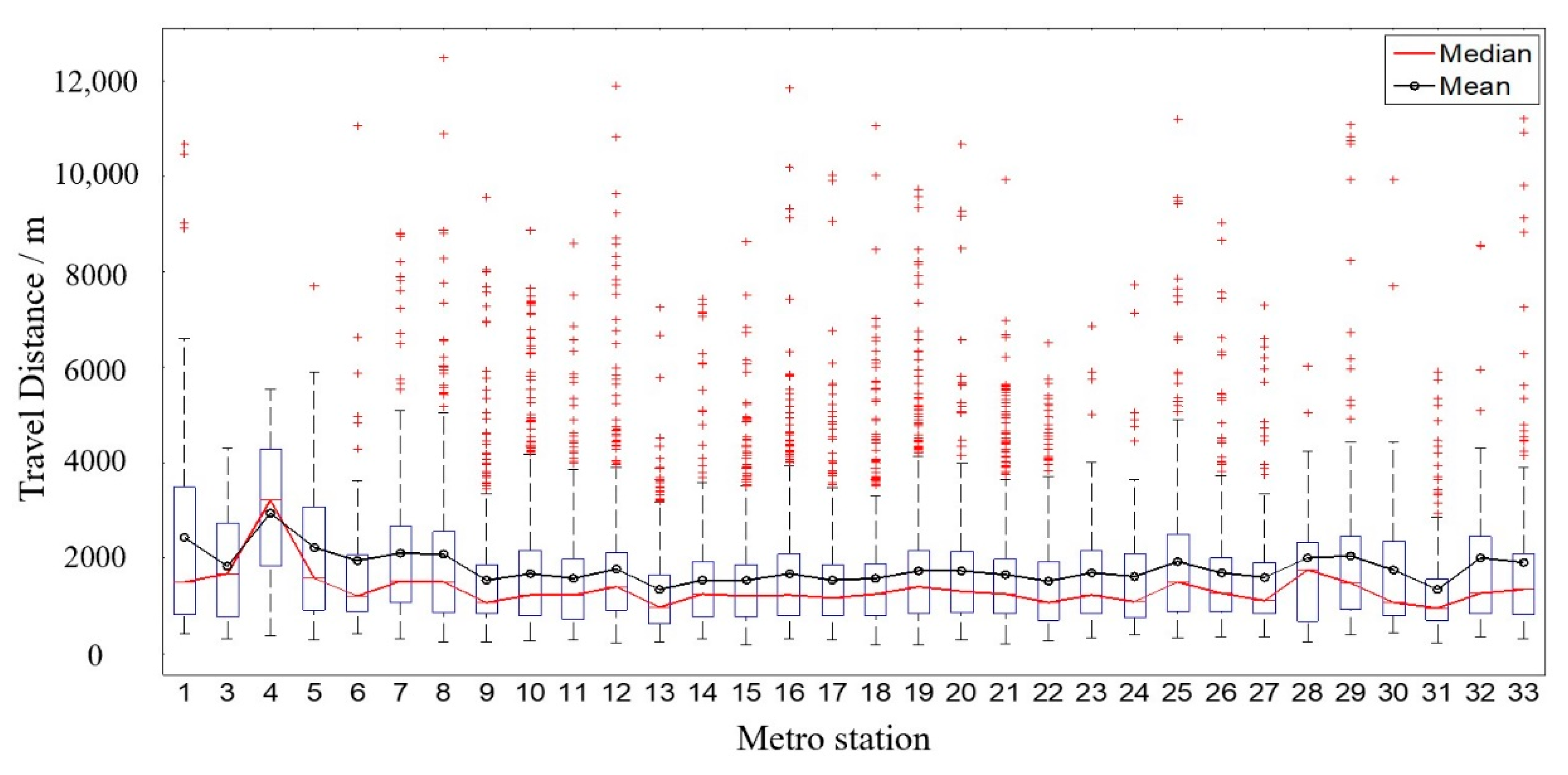
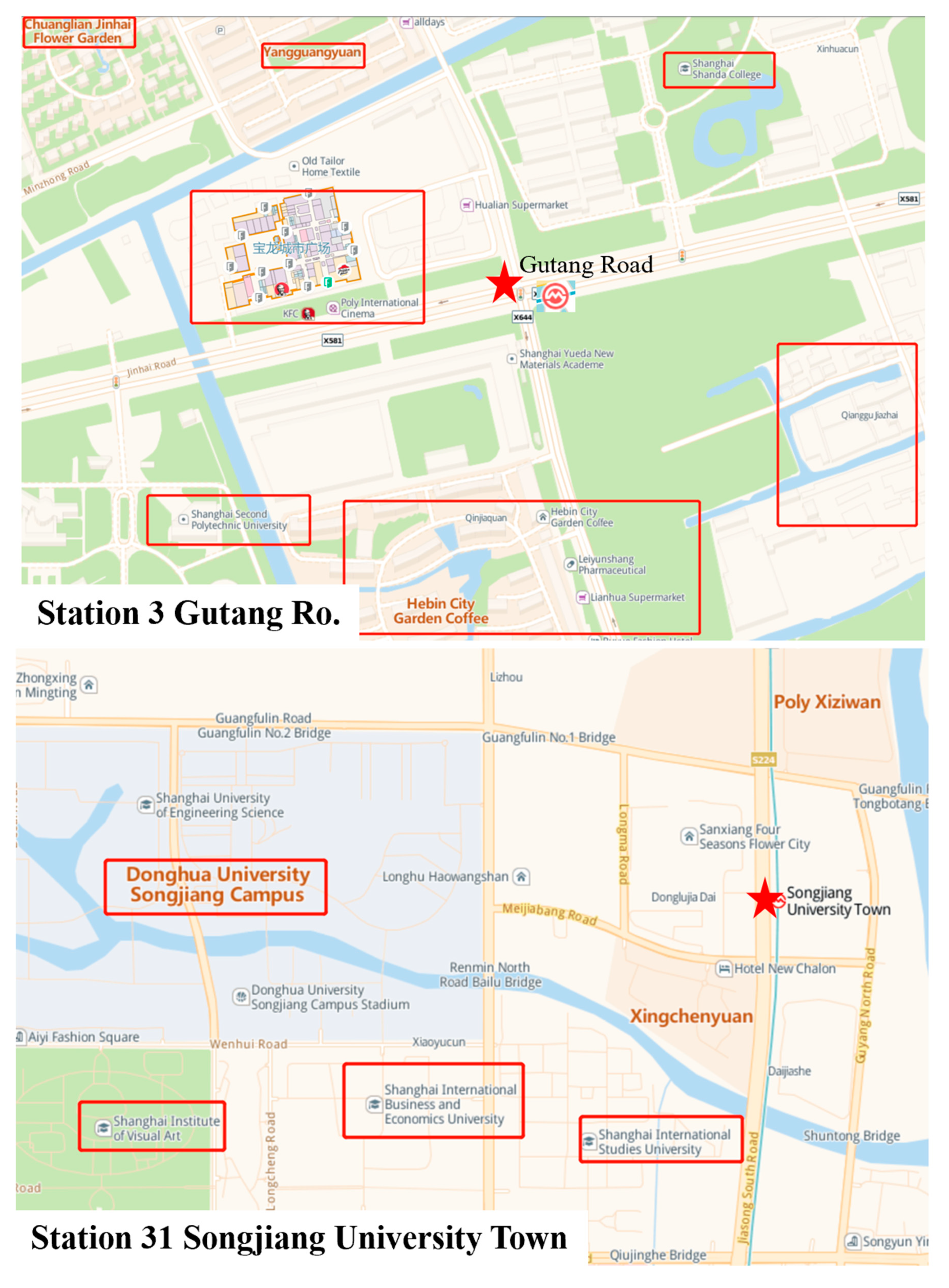
3.2. Usage Patterns of DLBS Near Stations in Different Area

As shown in Figure 1, Metro Line 9 has 35 stations and runs through downtown and into the suburbs. Agglomerative hierarchical clustering was applied to cluster stations of Metro Line 9 into different types based on the usage patterns of DLBS. GEV distribution was also implied to fit the travel distance distributions of clusters. The feature vectors were composed of the 25, 50, 75, and 90 percentiles and the mean value of travel distance distribution and the distance matrix was also constructed. Any usage of DLBS that begins or ends within 200 m of the metro station is relevant to the station. The total travel distance is composed of the travel distance of a cycling trip and distance between the sharing-bike and metro stations.

The travel distance distributions of DLBS near stations in different areas are shown in Figure 4. The data regarding stations 2, 34 and 35 are rejected due to too few observations. The median and mean values of travel distance fluctuate greatly. The result of clustering is shown in Figure 5. Three clusters are obtained. The Cluster 1 includes station 4; Cluster 2 contains the station 1, 5, 6, 7, 8, 28, 29, 32, and 33; Cluster 3 includes station 3, 9, 10, 11, 12, 13, 14, 15, 16, 17, 18, 19, 20, 21, 22, 23, 24, 25, 26, 27, 30, and 31. Different clusters are marked in Figure 1. Finally, two usage patterns of metro stations are distinguished excluding the exceptional case Cluster 1. Station 4 is divided into a separate category in Figure 5 and shows different characteristics in Figure 4. Using the map, it is observed that there are many factories around metro station 4 and a residential area is about 2.5 km away from metro station 4, which might be the reason for the different usage patterns of DLBS near station 4. This can also indicate that land use characteristics will affect the use of bicycles.

Stations in Cluster 2 are distributed at both ends of Metro Line 9, and Cluster 3 is distributed in the middle area. The area in the middle of line 9 is a densely populated downtown area, while the two ends are suburbs with a relatively smaller population. However, there are several suburban stations (stations 3, 30 and 31) that fall into Cluster 3. It might be ascribed to the fact that high density and high floating population nearby stations 3, 30, and 31. From the Map, it can be found that there are several universities, residential communities and commercial centers around these three metro stations. Figure 6 illustrates the land use around stations 3 and 31. Near the subway station 3, there are two universities, a large square and four residential areas marked by red rectangles. Similarly, near the subway station 31, four universities are marked by red rectangles. Therefore, these three stations have the same usage patterns as the stations in the city center because the land nearby is mainly for living and the surrounding population is highly concentrated.

To further explore the differences between Cluster 2 and Cluster 3, GEV distribution is applied to fit the travel distance of these two clusters. The fitting results are shown in Figure 7a,b. Cumulative density functions (CDF) of travel distance are shown in Figure 7c,d. It is worthy to note that travel distance always has an obvious right-skewed feature improving that the median of travel distance is always smaller than mean values. The location parameter $\mu$ and scale parameter $\sigma$ of the distributions are 1149.67 and 741.90 for Cluster 2, 995.739 and 582.56 for Cluster 3. 80% journeys using DLBS have travel distances less than 3 km in Cluster 2 while 80% journeys in Cluster 3 is less than 2.5 km. It indicates that the average travel distance of DLBS related to metro stations in areas of high population density is shorter than that of the areas with low population density. People in sparsely populated areas have the demand for a relatively long travel distance because land development is less intensive and people live in remote areas. Moreover, the scale parameter of Cluster 3 is bigger than that of Cluster 2. The larger the scale parameter is, the more spread out the distribution. The results suggest that the travel distance requirements of people using shared bikes in densely populated areas are more similar than those in scattered areas because the population is denser in places where land development is intensive.

In many cities, the public metro system and DLBS systems are important parts of the urban transportation system. Land development, use characteristics, and population aggregation in different areas of the city are different. The findings imply that the dispatching of shared bikes should be combined with urban planning. Bike-sharing companies can allocate bikes based on the usage characteristics of shared bikes near metro stations. If a metro station has a larger flow of people, but the number of shared bikes allocated here is small, then more shared bikes need to be configured nearby to meet the demand. Transportation managers should also consider the commercial DLBS systems in planning and management to facilitate people’s daily travel and alleviate the first-and-last mile problems. For example, companies are encouraged to adopt time-sharing systems to reduce the intensity of morning and evening peaks in cities. Improving the public transportation system near subway stations with long cycling distances is conducive to improving people’s commuting efficiency. According to the results of Shanghai, if there are many inhabitants around stations 2, 34 and 35, the operators of shared bikes can assignment more bikes around these stations. For the stations in Cluster 2, perhaps, transportation managers need to improve public transportations (e.g., bus) because of the long distance of biking.

4. Conclusions

In recent years, the dockless bike-sharing system rapidly develops and plays an indispensable role in urban public transport. This study explores the usage patterns of dockless bike-sharing to understand the principles of bike-sharing usage and support scientific planning of the bike-sharing system. The main findings can be summarized as follows:

(i)

The usage patterns of shared bikes at weekends and workdays are different. The usage of shared bikes presents an obvious ‘morning peak’ and ‘evening peak’ at workdays. On Saturday, however, there is only one peak at around 9:00 a.m. The demand for shared bikes shows two peaks on Sunday, but different from workdays. The peak in the afternoon of Sunday is significantly higher than that in the morning.

(ii)

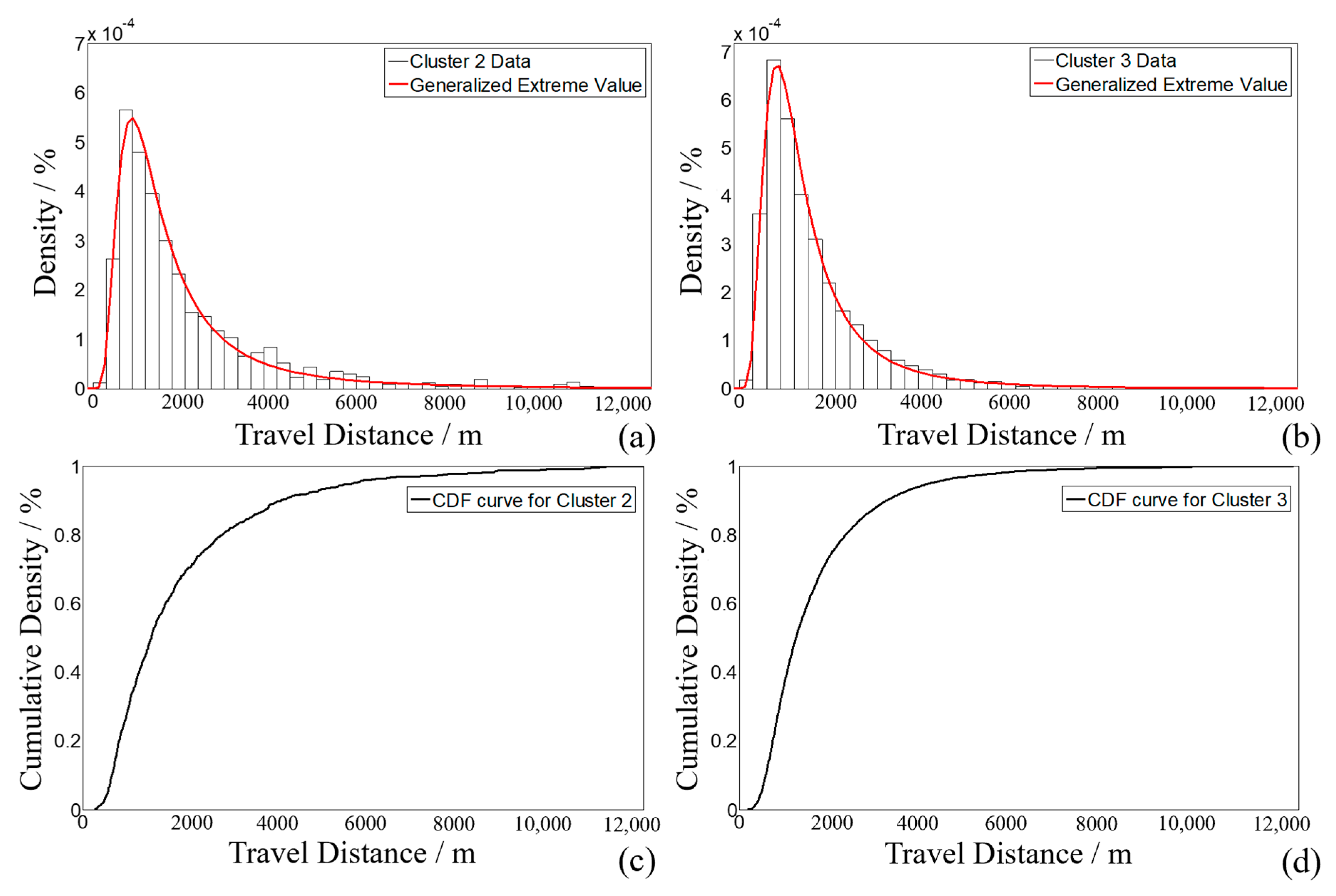
Type II (Fréchet distribution) of GEV distribution performs best in fitting travel distance. The average travel distance of weekends is longer than that of workdays.

(iii)

The agglomerative hierarchical clustering method was used to find the different usage patterns of DLBS linking to metro stations. Two distinct clusters with different usage patterns can be gained. The usage patterns of DLBS near stations in the suburbs and the urban areas are different. The results indicate that the land use characteristics around the metro station are important factors affecting the usage pattern of DLBS. Although the stations located in the suburbs, they have similar usage patterns with those in the urban areas because of the same land use characteristics.

(iv)

The average travel distance of DLBS related to metro stations in areas of high population density is shorter than that of the areas with low population density.

Although the usage characteristics of DBLS have been mined in the present paper, there are still some points that need to be studied in the future. Due to the limitation of data scope, we cannot study many influencing factors. If the data range is broad enough, the factors of weather, holidays and restricted areas could be taken into consideration. For clustering analysis, the features of point of interest (POI) around metro stations can be considered in the feature vector. The relationship between DLBS systems and bus stops can be studied in the future.

References

1. Demaio, P. Bike-sharing: History, impacts, models of provision, and future. J. Public Transp. 2009, 12, 41–56. [Google Scholar] [CrossRef]
2. Hatzopoulou, M.; Weichenthal, S.; Dugum, H.; Pickett, G.; Miranda-Moreno, L.; Kulka, R.; Andersen, R.; Goldberg, M. The Impact of Traffic Volume, Composition, and Road Geometry on Personal Air Pollution Exposures among Cyclists in Montreal, Canada. J. Expo. Sci. Environ. Epidemiol. 2013, 23, 46–51. [Google Scholar] [CrossRef] [PubMed]
3. Cervero, R. Transit-Oriented Development in the United States: Experiences, Challenges, and Prospects; Transportation Research Board: Washington, DC, USA, 2004. [Google Scholar]
4. Gao, K.; Sun, L.; Tu, H.; Li, H. Heterogeneity in Valuation of Travel Time Reliability and In-Vehicle Crowding for Mode Choices in Multimodal Networks. J. Transp. Eng. Part A Syst. 2018, 144, 04018061. [Google Scholar] [CrossRef]
5. Li, H.; Gao, K.; Tu, H. Variations in Mode-Specific Valuations of Travel Time Reliability and In-Vehicle Crowding: Implications for Demand Estimation. Transp. Res. Part A: Policy and Pract. 2017, 103, 250–263. [Google Scholar] [CrossRef]
6. GuangZhou Planning Bureau. The Case of Big Data Combined with City Planning. Available online: https://mp.weixin.qq.com/s?__biz=MzA3OTU3ODgxNA==&mid=2650583825&idx=1&sn=4a1e2f4df6d96e0d08ba639278f1da8e&chksm=87b940c0b0cec9d65ee7a76a0d25232d7811a83ab3858052d019bfb98780669aed6d4ed67139&mpshare=1&scene=23&srcid=0628YETa2Iyklv5UMuD51Exy#rd (accessed on 12 July 2019).
7. Shanghai Observer. The Stock of Shared Bikes in Shanghai Exceeds 1.7 Million. Why Are There Fewer than 2000 in This District? Available online: https://www.jfdaily.com/news/detail?id=64334 (accessed on 12 July 2019).
8. Li, W.; Tian, L.; Gao, X.; Batool, H. Effects of Dockless Bike-sharing System on Public Bike System: Case Study in Nanjing, China. In Proceedings of the 10th International Conference on Applied Energy (ICAE2018), Hong Kong, China, 2018. [Google Scholar]
9. Pfrommer, J.; Warrington, J.; Schildbach, G.; Morari, M. Dynamic Vehicle Redistribution and Online Price Ncentives in Shared Mobility Systems. IEEE Trans. Intell. Transp. Syst. 2014, 15, 1567–1578. [Google Scholar] [CrossRef] [Green Version]
10. Deng, L.; Xie, Y.; Huang, D. Bicycle-sharing Facility Planning Base on Riding Spatio-temporal Data. Planner 2017, 10, 82–88. [Google Scholar]
11. Du, Y.; Deng, F.; Liao, F. A Model Framework for Discovering the Spatio-temporal Usage Patterns of Public Free-floating Bike-sharing System. Transp. Res. Part C Emerg. Technol. 2019, 103, 39–55. [Google Scholar] [CrossRef]
12. Tao, T.; Guo, X.; Li, J.; Huang, Y. Operating Characteristics of a Public Bicycle-Sharing System Based on the Status of Stations: Case Study in Nanning City, China. Presented at 96th Annual Meeting of the Transportation Research Board, Washington, DC, USA, 2017. [Google Scholar]
13. Kou, Z.; Cai, H. Understanding Bike Sharing Travel Patterns: An Analysis of Trip Data from Eight Cities. Physica A 2019, 515, 785–797. [Google Scholar] [CrossRef]
14. Lv, X.; Pan, H. Sharing Bicycle Riding Characteristics Analysis in Shanghai Based on Mobike Opening Data. Shanghai Urban Plan. Rev. 2018, 02, 46–51. [Google Scholar]
15. Ma, X.; Ji, Y.; Jin, Y.; Wang, J.; He, M. Modeling the Factors Influencing the Activity Spaces of Bikeshare around Metro Stations: A Spatial Regression Model. Sustainability 2018, 10, 3949. [Google Scholar] [CrossRef] [Green Version]
16. Li, Y.; Zhu, Z.; Guo, X. Operating Characteristics of Dockless Bike-Sharing Systems near Metro Stations: Case Study in Nanjing City, China. Sustainability 2019, 11, 2256. [Google Scholar] [CrossRef] [Green Version]
17. Zhang, Z.; Qian, C.; Bian, Y. Bicycle–metro Integration for the ‘Last Mile’: Visualizing Cycling in Shanghai. Environ. Plan. A Econ. Space 2019, 51, 1420–1423. [Google Scholar] [CrossRef]
18. Zhao, P.; Li, S. Bicycle-Metro integration in a growing city: The Determinants of Cycling as a Transfer Mode in Metro Station Areas in Beijing. Transp. Res. Part A Policy Pract. 2017, 99, 46–60. [Google Scholar] [CrossRef]
19. Shen, Y.; Zhang, X.; Zhao, J. Understanding the Usage of Dockless Bike Sharing in Singapore. Int. J. Sustain. Transp. 2018, 12, 686–700. [Google Scholar] [CrossRef]
20. Zhang, Y.; Thomas, T.; Brussel, M.J.G.; Van Maarseveen, M.F.A.M. The Characteristics of Bike-sharing Usage: Case Study in Zhongshan, China. Int. J. Transp. Dev. Integr. 2018, 1, 245–255. [Google Scholar] [CrossRef]
21. Wilcoxon, F. Individual Comparisons by Ranking Methods. Biom. Bull. 1945, 1, 80–83. [Google Scholar] [CrossRef]
22. Jiang, B.; Yin, J.; Zhao, S. Characterizing the Human Mobility Pattern in a Large Street Network. Phys. Rev. E 2009, 80, 021136. [Google Scholar] [CrossRef] [PubMed] [Green Version]
23. Zhao, J.; Wang, J.; Deng, W. Exploring Bikesharing Travel Time and Trip Chain by Gender and Day of the Week. Transp. Res. Part C Emerg. Technol. 2015, 58, 251–264. [Google Scholar] [CrossRef]
Figure 1. Metro Line 9 in Shanghai, China.
Sustainability 12 00851 g001
Figure 2. (a1a5) represent the usage dynamic characteristics from Monday to Friday, respectively; (b,c) represent the usage dynamic characteristics of Saturday and Sunday, respectively.
Sustainability 12 00851 g002
Figure 3. (a,b) represent the probability density functions (PDF) of lognormal and GEV distribution for travel distance of workdays and weekends, respectively.
Sustainability 12 00851 g003
Figure 4. Travel distance characteristics around stations of Metro Line 9.
Sustainability 12 00851 g004
Figure 5. Dendrogram for features of travel distance around metro stations.
Sustainability 12 00851 g005
Figure 6. Land-use around stations 3 and 31, respectively.
Sustainability 12 00851 g006
Figure 7. (a,b) represent the probability density functions (PDF) of GEV distribution for travel distance of Cluster 2 and 3, respectively; (c,d) represent the cumulative density functions (CDF) of travel distance, respectively.
Sustainability 12 00851 g007