Article

Consequences of Spatial Heterogeneity of Forest Landscape on Ecosystem Water Conservation Service in the Yi River Watershed in Central China

1
Key Laboratory of Geospatial Technology for the Middle and Lower Yellow River Regions, Henan University, Ministry of Education, Kaifeng 475004, China
2
College of Environment and Planning, Henan University, Kaifeng 475004, China
3
Henan Research Academy of Environmental Protection Sciences, Zhengzhou 450003, China
*
Author to whom correspondence should be addressed.
Sustainability 2020, 12(3), 1170; https://doi.org/10.3390/su12031170
Submission received: 31 December 2019 / Revised: 21 January 2020 / Accepted: 4 February 2020 / Published: 6 February 2020

Abstract

:
Forest landscapes, especially their spatial heterogeneity, play a key role in sustaining the ecosystem water conservation service in a watershed. However, this domain has not been fully investigated. This study uses the Yi River watershed in central China as the study site. We calculated the water conservation amounts of different forests through the water balance method and quantified the landscape spatial heterogeneity of forests using landscape metrics. Then we ran correlation analysis to find the correlating relationship between the landscape spatial heterogeneity of forests and the ecosystem water conservation service. We finally applied a redundancy analysis to explore the respective influencing strength of the landscape compositional heterogeneity and configurational heterogeneity of forests on the water conservation service. Results indicate that: (1) The area proportion of different forests has a significant impact on the spatial distribution of the water conservation service. When mixed forest is dominant and its area proportion is much greater than that of other forests, the generation of the water conservation service can be best enhanced; (2) Changes of the landscape compositional heterogeneity and configurational heterogeneity of forests can affect the water conservation service to different degrees. In particular, the landscape spatial heterogeneity of mixed forest has the greatest impact on this ecosystem service; (3) The landscape configurational heterogeneity of deciduous broad-leaved forest and mixed forest has a greater impact on the water conservation service than the landscape compositional heterogeneity, whereas that of evergreen needle-leaved forest has the opposite effect. In general, appropriately adjusting the combination and configuration of different forests in a watershed can effectively promote the generation of the ecosystem water conservation service. This study provides a scientific basis for future forest management with a view to improving the landscape sustainability of forests.

1. Introduction

Forest is the most important terrestrial landscape that provides multiple ecosystem services (ESs), which include provisioning services, such as wood production; regulating services, such as climate regulation, air purification, and water conservation; cultural services, such as recreation; and supporting services, such as primary productivity [1,2,3,4,5,6]. An ecosystem water conservation service mainly reflects the roles of trees, shrubs, litter, and soil in the process of precipitation redistribution, thus conserving soil moisture, supplying underground water, regulating microclimates, decreasing surface dispersion, and regulating river flow [7]. It is an essential part of forest ecosystem functions. In China, forest is the main provider of the water conservation service. The amount of water conservation provided by forest has reached 743.23 billion m3, which accounts for about 61% of the total amount of water conservation in China [8]. Previous research has found that forest cover change is one of the most important direct driving forces for the water conservation services [7]. Forest cover is the service providing unit (SPU) of the water conservation service. The spatial and temporal change of landscape patterns can easily alter the SPU, therefore influencing the generation and maintenance of water conservation services [9,10,11]. Landscape spatial heterogeneity, which includes landscape compositional heterogeneity and configurational heterogeneity, is a specific aspect of changing landscape patterns. In addition, it is also the foundation and driving force of ecological processes and landscape functions and has an extremely close relationship to the continuous generation and steady provision of ESs [9,12]. However, research on the effects of forest landscape spatial heterogeneity on the water conservation service is still scarce [9,13,14,15].
Understanding how the spatial heterogeneity of forest landscapes affects the water conservation service is crucial. Exploring the relationship between landscape heterogeneity and ESs, and investigating under what circumstances landscape composition and configuration sustain or enhance these ESs, is also a process to consider for alternative forest management [15]. In this study, the theory of landscape ecology is applied to find out the consequences of the forest landscape spatial heterogeneity on the ecosystem water conservation service. Here we selected the Yi River watershed in China as the study area. We use water balance analysis to calculate the water conservation amount for different types of forests. Then we select and calculate the landscape metrics that can represent the landscape compositional heterogeneity and landscape configurational heterogeneity and compare these landscape metrics with the water conservation amount in each sub-watershed to reveal the relationship between them. Ordination analysis is also undertaken to explore the influencing strength of the forest landscape composition and landscape configuration on the water conservation service.
Our results show that the ability of different forests to generate and provide an ecosystem water conservation service is different. In this case, a growth of the area proportion of mixed forest can enhance the water conservation service. For each type of forest, a change in the landscape compositional heterogeneity and configurational heterogeneity can also affect the water conservation service to different degrees; for deciduous broad-leaved forest and mixed forest, the impact of their landscape configurational heterogeneity on the water conservation service is greater than that of their landscape compositional heterogeneity, but for evergreen needle-leaved forest, it is the opposite. Therefore we believe that changes in the spatial heterogeneity of forest landscapes could affect the spatial-temporal dynamics of some key resources, such as light, temperature, and water, which then affect forest ecosystem functions, adjusting the ability of forest ecosystem services. This study enriches the research on interactions between spatial heterogeneity, ecosystem functions, and the ecosystem services of forest landscapes. It provides a scientific foundation to the forest management on how to improve forest ecosystem functions and ecosystem services by adjusting the configuration of different forests, which has a profound significance.

2. Materials and Methods

2.1. Site Description

The Yi River is one of the major branches of the Yellow River in China. It flows from southwest to northeast and runs through Luanchuan County, Song County, Yichuan County, the Luolong District of Luoyang City, and Guxian Town of Yanshi City in the Henan Province of China. The overall length of its main stream is 237.4 km. Based on data from the Advanced Spaceborne Thermal Emission and Reflection Radiometer (ASTER) Global Digital Elevation Model (GDEM) Version 2 (overall accuracy of around 17 m at the 95% confidence level), we generated the extent of the Yi River watershed (111°19′~112°55′ E, 33°39′~34°41′ N) using the Soil and Water Assessment Tool (SWAT) in ArcMap 10.3 (Esri Inc., Redlands, CA, USA) (Figure 1). The total area of the Yi River watershed was 5933.34 km2, which can be categorized as a medium-sized watershed in China.
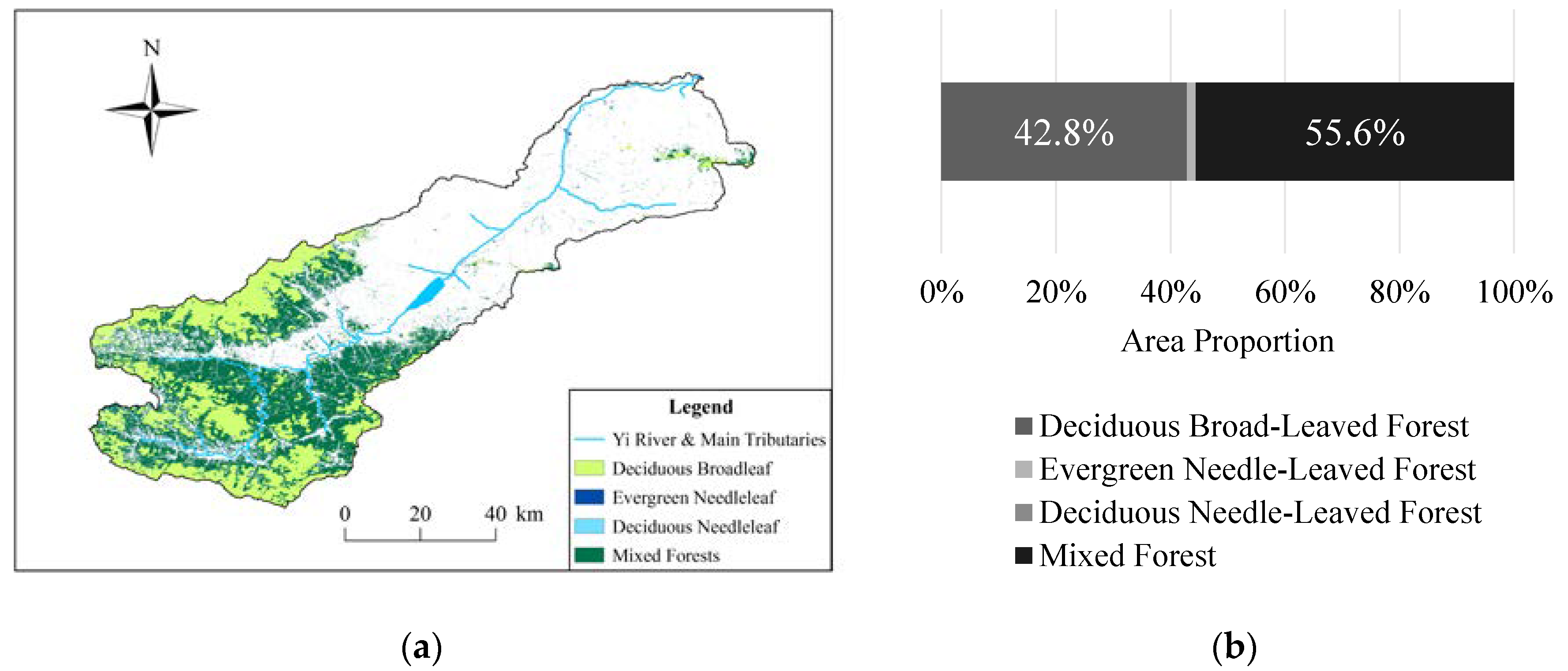
The Yi River watershed, as a study site, has typicality and is representative. It is located on the border of China’s warm temperate zone and north subtropical region and there is an obvious transition from southwest to northeast. Due to separation by mountains, the natural landforms in this watershed are mountainous area, hilly area, and valley. It forms a completely independent geographic unit with regional characteristics. With the interference of human activities, the land-cover types of the Yi River watershed are cropland, forest land, grassland, shrubland, wetland, impervious surface, and bare land. The total area of forest land is 2431.86 km2, which accounts for 41% of the total area of the Yi River watershed. The types of forests in this watershed include deciduous broad-leaved forest, evergreen needle-leaved forest, deciduous needle-leaved forest, and mixed forest (Figure 2a). Within this, mixed forest (55.6%) and deciduous broad-leaved forest (42.8%) are the dominant types. Evergreen needle-leaved forest accounts for only 1.6% of the total forest area, and the presence of deciduous needle-leaved forest is approximate to 0%, which is ignored in this study (Figure 2b).
The Yi River watershed is located in the arid region of China [16], therefore the soil evaporation is much greater than the precipitation. Historical records [17,18] show that the multi-year average precipitation in the Yi River watershed is 600 mm, while the multi-year average soil evaporation reaches up to 1790 mm. Nevertheless, Luanchuan County in the upper reaches is the rainstorm center of Henan Province, and the multi-year average precipitation can reach 850 mm. Depending on the “source–sink” landscape theory [19], the abundant rainfall and extensive forests make the upper reaches of the Yi River watershed become a “source” landscape for ecosystem water conservation services. Therefore, the Yi River watershed provides a suitable place for conducting this study.
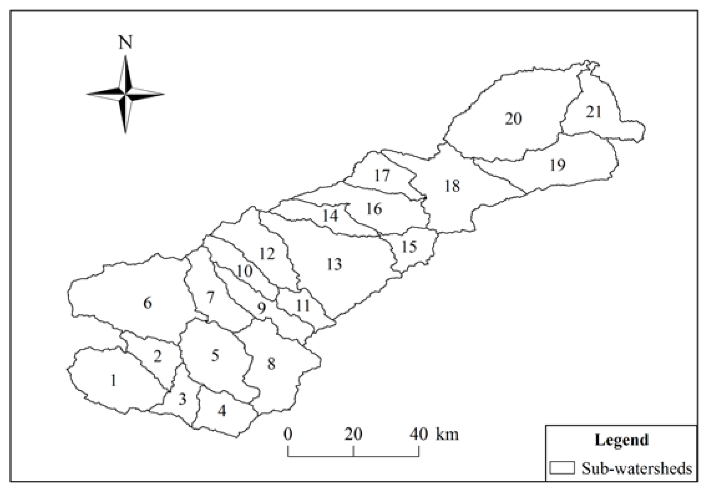
Combining remote sensing images and the topographic characteristics of the Yi River watershed, we used the watershed tool in ArcMap 10.3 (Esri Inc., Redlands, CA, USA) and categorized 21 typical sub-watersheds (Figure 3). According to the classifying criteria of the upper, middle, and lower reaches of the watershed, we classified sub-watersheds 1–11 as at the upper reaches, sub-watersheds 12–19 as at the middle reaches, and sub-watersheds 20–21 as at the lower reaches of the Yi River watershed.

2.2. Data Resources

Topographic data: Advanced Spaceborne Thermal Emission and Reflection Radiometer (ASTER) Global Digital Elevation Model (GDEM) Version 2 data were collected from the Ministry of Economy, Trade, and Industry (METI)—Earth Remote Sensing Data Analysis Centre (ERSDAC) in Japan and from the National Aeronautics and Space Administration (NASA)—Earth Observing System (EOS)—Data Information System (EOSDIS)—Land Processes (LP)—Distributed Active Archive Centre (DAAC) in the United States.
Landscape data: the forest land-cover data (30 m spatial resolution) were collected from the Finer Resolution Observation and Monitoring of Global Land Cover (FROM-GLC) established by Tsinghua University. These data were generated by remote sensing images from Landsat Thematic Mapper (TM) and Enhanced Thematic Mapper Plus (ETM+) data [20].

2.3. Methods

2.3.1. Quantifying an Ecosystem Water Conservation Service

There are numerous ways to calculate amounts of water conservation, such as comprehensive water storage capacity analysis, precipitation storage analysis, residue of canopy interception analysis, water balance analysis, multi-factor regression analysis, forest hydrological modeling analysis, and multi-model integration analysis [21,22]. Here we selected water balance analysis to calculate the water conservation amounts in the Yi River watershed. The water balance method is a widely used theoretical method [22]. It treats a forest ecosystem as a “black box” and focuses on the input and output amounts of water. We assumed that the total amount of water was balanced, therefore the difference between the input and output is the water conservation amount of this ecosystem. The calculating formula is
W = (R − E) × A = θR × A
where W is the water conservation amount (m3 per year), R is the annual average precipitation (mm), E is the annual average evapotranspiration (mm), A is the total area of the study site (or ecosystem) (hm2), and θ is the runoff coefficient.
The annual average precipitation in the Yi River watershed was 864.4 mm in 2017. From the historical and statistical data, it is known that the evapotranspiration of the Yi River watershed is much greater than its precipitation [17,18]. Especially in winter, the evapotranspiration is even five times greater than the precipitation. Therefore we used the runoff coefficient to calculate the water conservation amount. The formula is
θ = D/P
where θ is the runoff coefficient, D is the depth of runoff (mm), and P is the depth of precipitation (mm).
All the runoff coefficients were obtained from the published literature and monographs [23,24] (Table 1). We calculated the annual average precipitation per unit area by dividing the annual average precipitation by the total area of the Yi River watershed, and the result was 0.15 mm/km2. Then we multiplied the area of each type of forest to get the annual average precipitation of these forests. Finally, we got the water conservation amount of each type of forest using Formula (1).

2.3.2. Analyzing Landscape Spatial Heterogeneity

Landscape metrics can quantify the landscape composition and configuration of land-cover types [25]. We calculated the landscape metrics of the different forests in each sub-watershed at class level using FRAGSTATS 4.2 (UMass Landscape Ecology Lab., Amherst, MA, USA). According to the software instructions, we selected the landscape metrics of total (class) area (CA), percentage of landscape (PLAND), largest patch index (LPI), number of patches (NP), contiguity index (CONTIG), patch cohesion index (COHESION), aggregation index (AI), and landscape division index (DIVISION) (Table 2). Wherein the CA, PLAND, and LPI can reflect landscape composition change, whereas NP, CONTIG, COHESION, AI, and DIVISION can reflect landscape configuration change.

2.3.3. Statistical Analysis

We used correlation analysis to find out the relationship between forest landscape metrics and the amount of water conservation. Then we applied a redundancy analysis (RDA) to compare the influencing strength of forest landscape composition and configuration on the ecosystem water conservation service. Before undertaking the RDA, we completed a detrended correspondence analysis (DCA) to calculate the gradient and length of the sort axis. Our DCA result was less than 3, meaning that a RDA could be applied in this study. These statistical analyses were conducted using the Statistical Product and Service Solutions (SPSS) 20.0 (IBM, Armonk, NY, USA) and Canoco 4.5 software (Wageningen University and Research, Wageningen, the Netherlands), respectively.

3. Results and Discussion

3.1. Spatial Distribution of the Water Conservation Service

We calculated the total water conservation amount that was provided by different forests for each sub-watershed. Due to the total amount of water conservation being influenced by the area of the sub-watershed, we calculated the water conservation amount per unit area of each sub-watershed. According to this value, we categorized the water conservation service into four levels by quantile using ArcMap 10.3 (Esri Inc., Redlands, CA, USA), to show the degree of importance of each sub-watershed to this ES (Figure 4).
Generally, the spatial distribution for different forests that generate and provide the water conservation service in the Yi River watershed showed a downward trend from the upper reaches to the lower reaches. Comparing the distribution of the area proportion of different forests in each sub-watershed, we found that when deciduous broad-leaved forest and mixed forest are dominant (the total area proportion is over 95%) and the area occupied by mixed forest was over two times larger than that of deciduous broad-leaved forest, the capacity for providing the water conservation service was the greatest. When the area occupied by these two forests was nearly half and half, the capacity for providing the water conservation service declined, whereas when the area occupied by deciduous broad-leaved forest was much greater than mixed forest, the capacity for providing the water conservation service was the lowest. When deciduous broad-leaved forest, evergreen needle-leaved forest, and mixed forest were dominant, the capacity for providing the water conservation service was greater than that of the third case mentioned above. From this, it is obvious that in a certain region, the combination and area proportion of different forests can strongly influence the amount of water conservation. In the subsequent study, we emphatically discuss which type of forest influences the water conservation service more and what kind of combination of different forests promote this ES.

3.2. Variations of Spatial Heterogeneity in Forest Landscape

3.2.1. Landscape Compositional Heterogeneity

We analyzed landscape metrics that represent landscape compositions of deciduous broad-leaved forest, evergreen needle-leaved forest, and mixed forest in each sub-watershed.
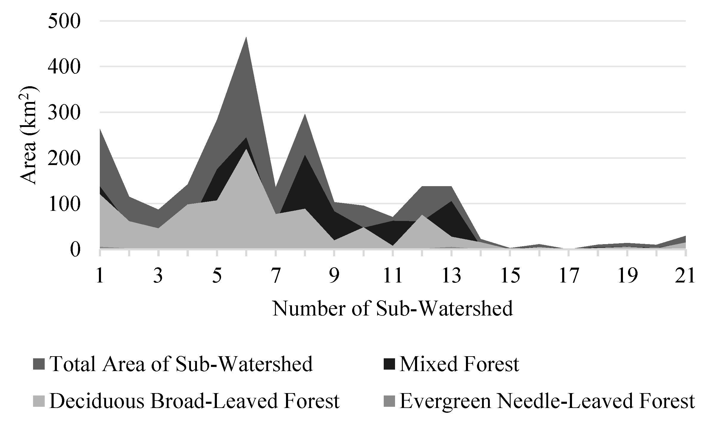
Results showed that the total areas of mixed forest and deciduous broad-leaved forest have a similar variation trend for the total area of forests in each sub-watershed from the upper reaches to the lower reaches, whereas the CA of evergreen needle-leaved forest was too small to see its variation (Figure 5).
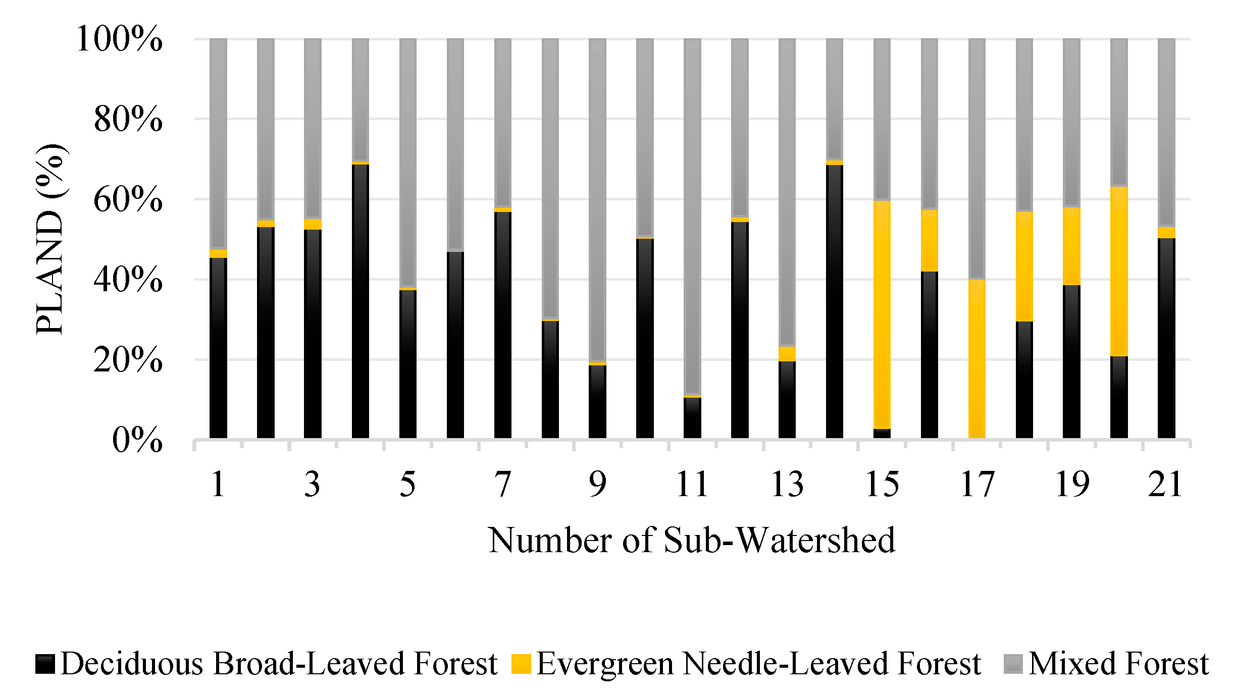
In the upper reaches, deciduous broad-leaved forest and mixed forest were dominant; the area proportions of evergreen needle-leaved forest in each sub-watershed were all lower than 3%. In the bottom of the middle reaches and the top of the lower reaches, the area proportions of evergreen needle-leaved forest in each sub-watershed were much greater, especially in sub-watershed 15 where the PLAND of evergreen needle-leaved forest was over 50% (Figure 6).
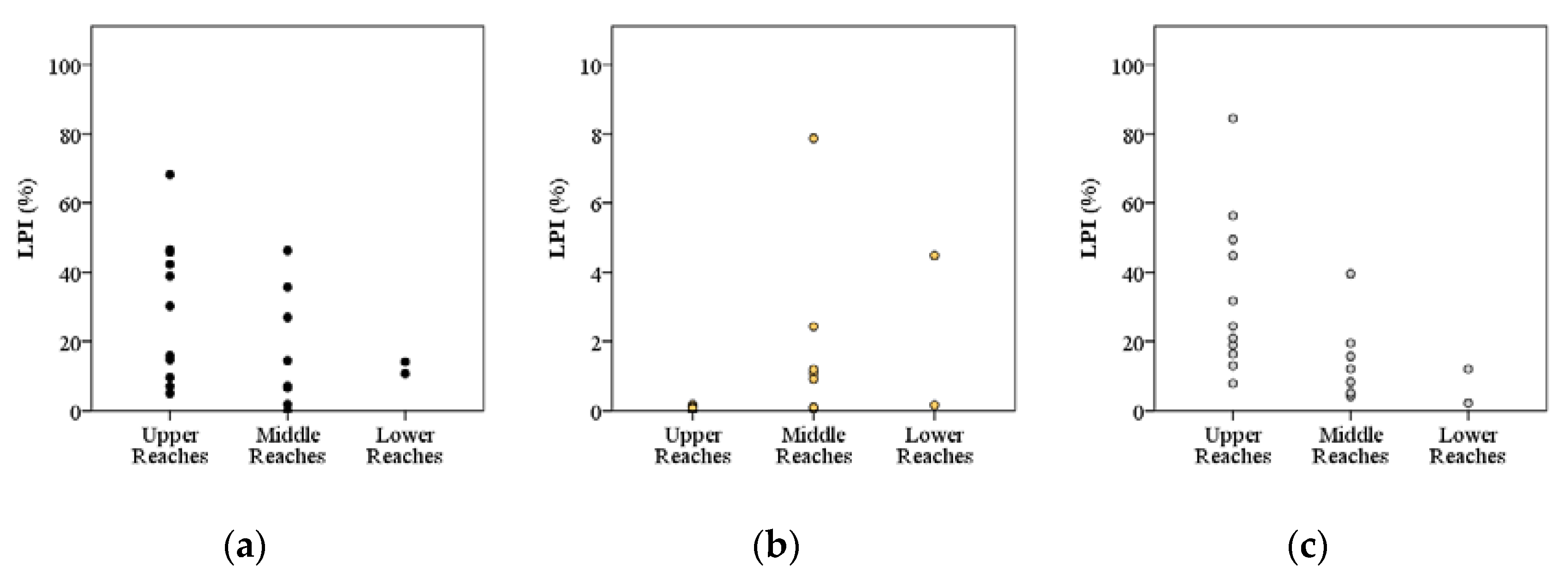
We analyzed the proportion of the largest patch of different forests in the upper, middle, and lower reaches, respectively. Generally, the dispersion of LPI values of deciduous broad-leaved forest diminished from the upper reaches to the lower reaches (Figure 7a), the LPI of evergreen needle-leaved forest was no more than 10% in each sub-watershed, and the dispersion of LPI was lowest in the upper reaches (lower than 1%) (Figure 7b). The dispersion of LPI values of mixed forest had a similar trend to that of deciduous broad-leaved forest (Figure 7c).
CA, PLAND, and LPI are all metrics that can represent landscape compositional heterogeneity. We can conclude form the results that from the upper reaches to the lower reaches of the Yi River watershed, the big patches of deciduous broad-leaved forest and mixed forest split into smaller ones, and the patch area gets smaller so that their landscape compositional heterogeneity decreases; whereas for evergreen needle-leaved forest, small patches merge together to form larger patches. The area of this type of forest also increases, and therefore its landscape compositional heterogeneity generally increases.

3.2.2. Landscape Configurational Heterogeneity

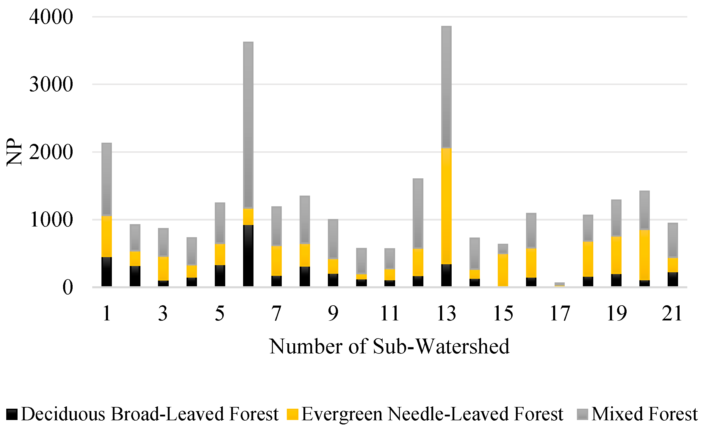
We analyzed landscape metrics that represent landscape configuration. NP indicates the amount of patches of forest in each sub-watershed. A greater quantity of patches shows that the degree of landscape fragmentation was higher. The total NP of all forests in sub-watershed 6 and 13 was the highest, while that of sub-watershed 17 was the lowest. Generally, the degree of landscape fragmentation of forests gradually increased from the upper reaches to the lower reaches, especially that of evergreen needle-leaved forest (Figure 8).
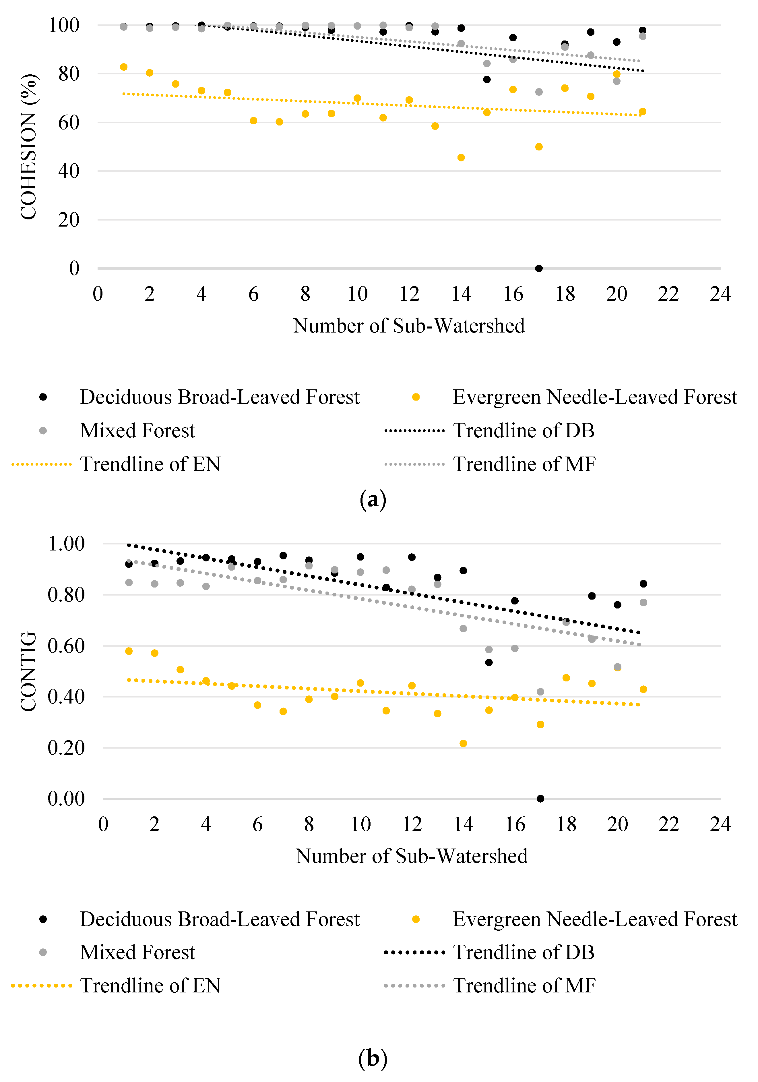
COHESION values of deciduous broad-leaved forest, evergreen needle-leaved forests, and mixed forest had downward trends from the upper reaches to the lower reaches. Therefore, the COHESION of deciduous broad-leaved forest and mixed forest was higher than that of evergreen needle-leaved forest, which means the connectivity of patches of the first two forests was better than the latter one (Figure 9a).
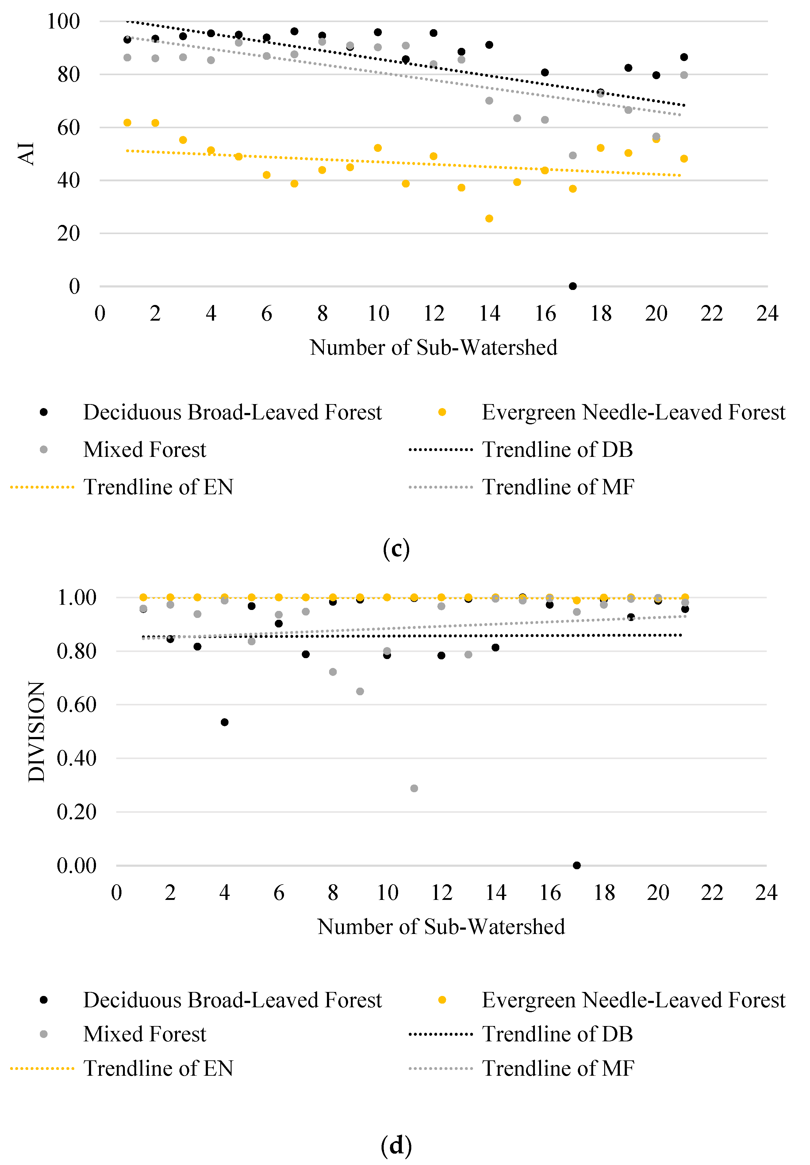
The variation tendencies of CONTIG and AI were similar (Figure 9b,c). In the upper reaches, the CONTIG of deciduous broad-leaved forest and mixed forest was above 0.8, and their AI values were above 80%. This means patches of these two forests were adjacent with a high degree of aggregation. In the middle and lower reaches, the values of landscape metrics decreased, therefore the patches of forests were less adjacent, and the degree of aggregation declined. CONTIG and AI values of evergreen needle-leaved forest declined with a smaller amplitude. Patches of evergreen needle-leaved forest were less adjacent with a lower degree of aggregation.
The DIVISION of deciduous broad-leaved forest and mixed forest showed a higher possibility that two random pixels were not in the same patch in the middle and lower reaches, which means the degree of fragmentation of these two forests increased from the upper reaches to the lower reaches of the watershed. DIVISION values of evergreen needle-leaved forest were close to 1, meaning that the distribution of patches of evergreen needle-leaved forest were dispersive, and the degree of fragmentation was high (Figure 9d).
From the statistics of the above landscape metrics, it was obvious that the degree of fragmentation of forests increased from the upper reaches to the lower reaches. This means the connectivity of different types of forests had a declining trend. Patches of forests got smaller, and the aggregation degree also decreased. The upward degree of fragmentation signified that the configurational heterogeneity of forests rose, and therefore the landscape configurational heterogeneity was enhanced.

3.3. Correlation between Forest Landscape Spatial Heterogeneity and the Ecosystem Water Conservation Service

The results of Spearman correlating analysis indicated that the landscape composition metrics of different forests had dissimilar correlations with the total amount of water conservation in each sub-watershed (Table 3). The CA of deciduous broad-leaved forest had a significant positive correlation (p < 0.01) with the amount of water conservation, whereas the PLAND and LPI had no significant correlating relationships with the amount of water conservation. For evergreen needle-leaved forest, there were strong negative correlations (p < 0.01) between the PLAND and LPI and the amount of water conservation. All the landscape composition metrics of mixed forest had positive correlations with the amount of water conservation, wherein the correlation between the CA and the amount of water conservation is much stronger (p < 0.01) than other landscape metrics (p < 0.05).
We can conclude from the result that the water conservation service can be strongly affected by a change of forest landscape composition. Meanwhile, the landscape composition of different forests can impact the water conservation service differently. For deciduous broad-leaved forest, enlarging the total area can effectively improve the amount of water conservation, but when the area proportion or the largest patch area is increased, it does not necessarily contribute to the water conservation service. For evergreen needle-leaved forest, increasing the area proportion and largest patch area may not promote the generation of the water conservation service. That is, the decrease of landscape compositional heterogeneity of evergreen needle-leaved forest may cause negative consequences to the ecosystem water conservation service. For mixed forest, any change in the landscape compositional heterogeneity can affect the water conservation service. When the landscape compositional heterogeneity decreases, the water conservation service that is provided by mixed forest can be effectively improved.
Landscape configuration metrics of deciduous broad-leaved forest, such as the NP, CONTIG, COHESION, and AI, had significant positive correlations (p < 0.01) with the total amount of water conservation, whereas DIVISION showed no significant correlating relationship with the water conservation service (Table 4). On the contrary, the DIVISION of evergreen needle-leaved forest had a very strong significant positive correlation (p < 0.01) with the amount of water conservation, but other landscape configuration metrics had no significant correlating relationship with this ES (Table 5).
All of the landscape configuration metrics of mixed forest correlated significantly with the total amount of water conservation. From these metrics, the NP, CONTIG, COHESION, and AI showed significant positive correlations (p < 0.01) with the amount of water conservation, while the DIVISION showed a significant negative correlation (p < 0.01) with the amount of water conservation (Table 6).
From the results, it can be concluded that when patches of deciduous broad-leaved forest are more aggregated, or the connectivity among the patches is higher, the landscape configurational heterogeneity of this type of forest is low, which can contribute to sustaining the water conservation service. However, for evergreen needle-leaved forest, it is just the reverse. Only when the patches of evergreen needle-leaved forest are more dispersive is the amount of water conservation likely to be improved. Vice versa, for mixed forest, there is strong evidence that when the landscape configurational heterogeneity decreases, the water conservation service that is provided by this type of forest is enhanced.

3.4. The Influencing Strength of Forest Landscape Spatial Heterogeneity on the Water Conservation Service

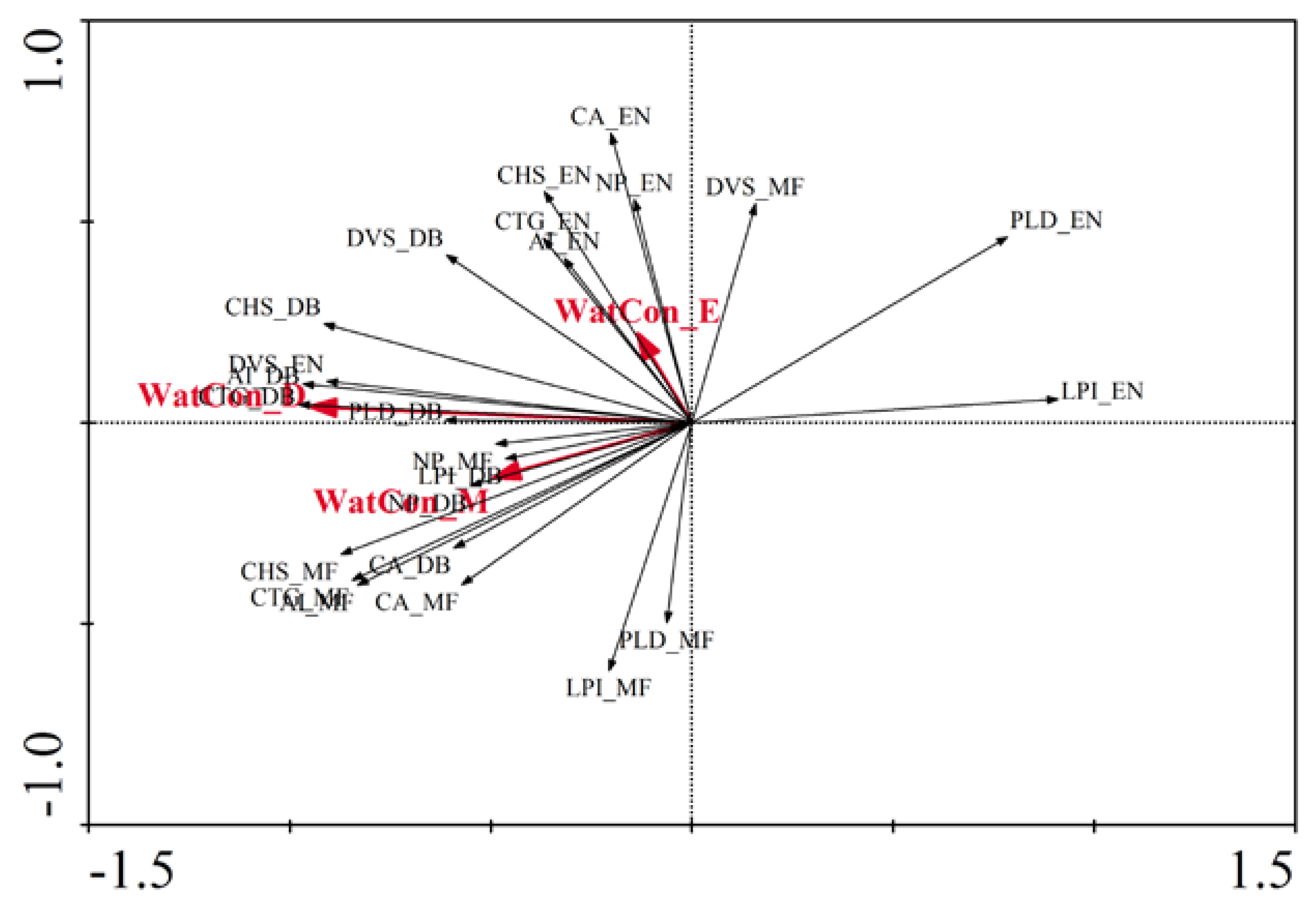
In the RDA, we selected the water conservation amount of different forests and their relative landscape metrics. The RDA results indicated that the cumulative contribution rates of axis 1 and axis 2 reached 97%, which means a RDA can effectively reflect the relationship between the amount of water conservation and landscape metrics (Table 7).
The correlation between the ecosystem service and landscape metrics and the influencing strength of the landscape metrics on the ecosystem service are mainly determined by the included angle cosine and the arrow length of indicators. When the included angle between two indicators is less than 90°, their correlation is positive, whereas when the included angle between two indicators is greater than 90°, their correlation is negative. The arrow length represents the proportion of the impacting factor. The longer the arrow is, the greater the influencing strength of the impacting factor is.
For deciduous broad-leaved forest, the water conservation service provided by the forest is positively related to the CA, NP, CONTIG, COHESION, and AI. The influencing strength from these landscape metrics on the water conservation service is CONTIG > AI > COHESION > CA > NP (Figure 10). Therefore, a change of landscape configurational heterogeneity can affect the water conservation service much more strongly than a change of landscape compositional heterogeneity. The way in which patches are configured and combined decides their aggregating degree and the connectivity between them, and the effects of these factors on the water conservation service are much larger than the effects of factors such as the total area and number of patches of deciduous broad-leaved forest on the water conservation service.
The water conservation service provided by evergreen needle-leaved forest was positively related to the DIVISION and negatively related to the PLAND and LPI. The ordination results show that the influencing strength of these landscape metrics was similar (Figure 10). The influencing strength of these landscape metrics on the water conservation service was PLAND > LPI > DIVISION, which means the change of landscape compositional heterogeneity of evergreen needle-leaved forest impacted on the water conservation service much more strongly. In other words, the effects of area and the proportion of patches on the water conservation service was greater than that of the configuration and combination among patches.
The water conservation service provided by mixed forest was positively correlated to the CA, PLAND, LPI, NP, CONTIG, COHESION, and AI, and negatively correlated to the DIVISION. The influencing strength of these landscape metrics on water conservation service was CONTIG > COHESION > AI > CA > LPI > DIVISION > PLAND > NP (Figure 10). The ordination obviously showed that the impact of the landscape configurational heterogeneity of mixed forest on the water conservation service was much greater than the landscape compositional heterogeneity.

4. Conclusions

The spatial heterogeneity of forest landscapes and the ecosystem water conservation service are closely related. Variation of landscape spatial heterogeneity can significantly affect the generation and maintenance of the water conservation service. In our study, we found that: (1) the area proportion of different forests has a significant impact on the spatial distribution of the water conservation service. When mixed forest is dominant and its area proportion is much greater than that of other forests, the generation of the water conservation service can be best enhanced; (2) Changes of the landscape compositional heterogeneity and configurational heterogeneity of forests can affect the water conservation service to different degrees. In particular, the landscape spatial heterogeneity of mixed forest has the greatest impact on this ecosystem service; (3) The landscape configurational heterogeneity of deciduous broad-leaved forest and mixed forest has a greater impact on the water conservation service than the landscape compositional heterogeneity, whereas for evergreen needle-leaved forest the effects are opposite. These findings demonstrate that appropriately adjusting the combination and configuration of different types of forests can effectively promote the generation of the ecosystem water conservation service. For example, improving the area proportion of mixed forest is the most effective way to enhance the water conservation service in this case.
To explore the relationship and potential mechanisms between the spatial heterogeneity of forest landscapes and the ES is also a process to consider for alternative forest management. This is because changes in the spatial heterogeneity of forest landscapes can affect the dynamics of some key resources (light, temperature, water etc.) and thus impact on the interactions between trees and, in the end, the forest dynamics, functioning, and ecosystem services. In forest management, considering the configuration of different forests can effectively sustain and promote the ability of forests to generate ESs. An ecosystem water conservation service is closely related to the canopy of different types of forests. Increasing canopy interception can contribute to the generation of a water conservation service. Therefore, the decision maker can depend on research results to appropriately adjust the configuration of different forests for improving the water conservation service, such as reducing the landscape configurational heterogeneity of deciduous broad-leaved forest, merging small patches to make these forests more aggregate, improving the connectivity among the patches, or decreasing the total area and area of the largest patches of evergreen needle-leaved forest.
This study enriches the investigation of the spatial heterogeneity of forest landscape and forest ecosystem services and deepens our understanding of the ecological mechanisms that underpin these relationships. It provides a scientific foundation for future forest management from the perspective of landscape ecology and is aimed to improve the sustainability of forest landscape, and thus sustain and generate a more high-quality ESs.

Author Contributions

Conceptualization, S.D., L.L., and Z.B.; data curation, L.L.; formal analysis, L.L.; investigation, L.L. and Z.B.; methodology, L.L. and S.D.; project administration, S.D.; resources, L.L. and Z.B.; software, L.L. and Z.B.; supervision, S.D.; validation, L.L. and S.D.; visualization, L.L. and Z.B.; writing―original draft, L.L.; writing―review and editing, Z.B. and S.D. All authors have read and agree to the published version of the manuscript.

Funding

This research was funded by the National Natural Science Foundation of China, grant number 41771202.

Conflicts of Interest

The authors declare no conflict of interest.

References

  1. Bai, J.; Peng, D.; Yu, X.; Zheng, X. Research advances in forest landscape ecology. Chin. J. Ecol. 2005, 24, 943–947. [Google Scholar]
  2. Guo, J.; Zhang, Y. Advances and perspective of forest landscape ecology in China. World For. Res. 2003, 16, 46–49. [Google Scholar]
  3. Tiemann, A.; Ring, I. Challenges and opportunities of aligning forest function mapping and ecosystem service concept in Germany. Forests 2018, 9, 691. [Google Scholar] [CrossRef] [Green Version]
  4. Caputo, J.; Butler, B. Ecosystem service supply and capacity on U.S. family forestlands. Forests 2017, 8, 395. [Google Scholar] [CrossRef] [Green Version]
  5. Williams, K.; Biedenweg, K.; Cerveny, L. Understanding ecosystem service preferences across residential classifications near Mt. Baker Snoqualmie National Forest, Washington (USA). Forests 2017, 8, 157. [Google Scholar] [CrossRef] [Green Version]
  6. Millenium Ecosystem Assessment. Ecosystems and Human Well-Being: Synthesis; Island Press: Washington, DC, USA, 2005. [Google Scholar]
  7. Gong, S.; Xiao, Y.; Xiao, Y.; Zhang, L.; Ouyang, Z. Driving forces and their effects on water conservation services in forest ecosystems in China. Chin. Geogr. Sci. 2017, 27, 216–228. [Google Scholar] [CrossRef] [Green Version]
  8. Gong, S.; Xiao, Y.; Zheng, H.; Xiao, Y.; Ouyang, Z. Spatial patterns of ecosystem water conservation in China and its impact factors analysis. Acta Ecol. Sin. 2017, 37, 2455–2462. [Google Scholar]
  9. Liu, L.; Bian, Z.; Ding, S. Effects of landscape spatial heterogeneity on the generation and provision of ecosystem services. Acta Ecol. Sin. 2018, 38, 6412–6421. [Google Scholar]
  10. Anderssona, E.; McPhearson, T.; Kremer, P.; Gomez-Baggethun, E.; Haase, D.; Tuvendal, M.; Wurster, D. Scale and context dependence of ecosystem service providing units. Ecosyst. Serv. 2015, 12, 157–164. [Google Scholar] [CrossRef]
  11. Blumstein, M.; Thompson, J.R. Land-use impacts on the quantity and configuration of ecosystem service provisioning in Massachusetts, USA. J. Appl. Ecol. 2015, 52, 1009–1019. [Google Scholar] [CrossRef]
  12. Liu, L.; Liu, H.; Ren, J.; Bian, Z.; Ding, S. Research progress on the mechanism of ecosystem services generation. Chin. J. Appl. Ecol. 2017, 28, 2731–2738. [Google Scholar]
  13. Roces-Díaz, J.V.; Vayreda, J.; Banqué-Casanovas, M.; Díaz-Varela, E.; Bonet, J.A.; Brotons, L.; de-Miguel, S.; Herrando, S.; Martínez-Vilaltaah, J. The spatial level of analysis affects the patterns of forest ecosystem services supply and their relationships. Sci. Total Environ. 2018, 626, 1270–1283. [Google Scholar] [CrossRef] [PubMed] [Green Version]
  14. Qiu, J.X.; Turner, M.G. Importance of landscape heterogeneity in sustaining hydrologic ecosystem services in an agricultural watershed. Ecosphere 2015, 6, 1–19. [Google Scholar] [CrossRef]
  15. Turner, M.G.; Donato, D.C.; Romme, W.H. Consequences of spatial heterogeneity for ecosystem services in changing forest landscapes: Priorities for future research. Landsc. Ecol. 2013, 28, 1081–1097. [Google Scholar] [CrossRef]
  16. Yang, J.P.; Ding, Y.J.; Chen, R.S.; Liu, L.Y. Variations of precipitation and evaporation in north China in recent 40 years. J. Arid Land Resour. Environ. 2003, 17, 6–11. [Google Scholar]
  17. Wang, W.T.; Qian, L.X. Spatial distribution and seasonal variation of evapotranspiration in Yiluo River basin based on MODIS data. Resour. Sci. 2012, 34, 1582–1590. [Google Scholar]
  18. Wang, W.T.; Wang, J.L.; Du, J. Land surface evaporation estimation of Yiluo River basin based on fusion of ETM+ and MODIS data. Geogr. Res. 2013, 32, 817–821. [Google Scholar]
  19. Chen, L.D.; Fu, B.J.; Zhao, W.W. Source-sink landscape theory and its ecological significance. Acta Ecol. Sin. 2006, 26, 1444–1449. [Google Scholar] [CrossRef]
  20. Li, C.; Wang, J.; Hu, L.; Yu, L.; Clinton, N.; Huang, H.; Yang, J.; Gong, P. A circa 2010 thirty meter resolution forest map of China. Remote Sens. 2014, 6, 5325–5343. [Google Scholar] [CrossRef] [Green Version]
  21. Hou, X.; Sun, W.; Li, J.; Li, Q. The progress of research and forecast on the quantification of the forest water conservation capacity. J. Arid Land Resour. Environ. 2018, 32, 121–127. [Google Scholar]
  22. Zhang, B.; Li, W.; Xie, G.; Xiao, Y. Water conservation function and its measurement methods of forest ecosystem. Chin. J. Ecol. 2009, 28, 529–534. [Google Scholar]
  23. Tian, Y.; Li, M.; Wu, B. The land use dynamics simulation and water conservation service capacity estimates in Beibu Gulf Coastal—A case study in Qinzhou City of Guangxi Zhuang Autonomous region. Yunnan Geogr. Environ. Res. 2013, 25, 69–78. [Google Scholar]
  24. Xie, G.; Lu, C.; Leng, Y.; Zheng, D.; Li, S. Ecological assets valuation of the Tibetan Plateau. J. Nat. Resour. 2003, 18, 189–196. [Google Scholar]
  25. Gustafson, E.J. Quantifying landscape spatial pattern: What is the state of the art? Ecosystems 1998, 1, 143–156. [Google Scholar] [CrossRef]
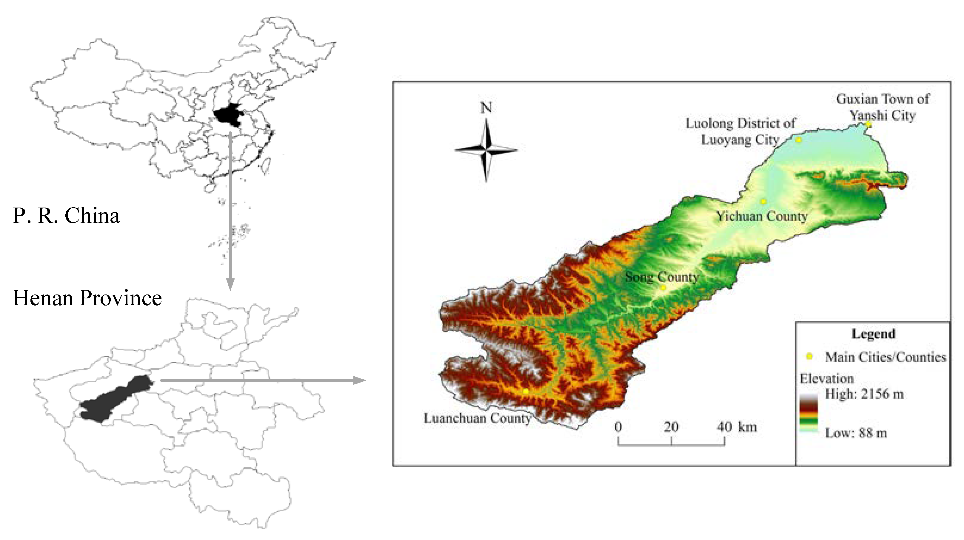
Figure 1. Location and topographic map of the Yi River watershed.
Sustainability 12 01170 g001
Figure 2. (a) Forest map of the Yi River watershed and (b) the area proportion of each forest type.
Sustainability 12 01170 g002
Figure 3. The partition of typical sub-watersheds in the Yi River watershed.
Sustainability 12 01170 g003
Figure 4. Spatial distribution of the ecosystem water conservation service.
Sustainability 12 01170 g004
Figure 5. Statistics of the landscape metric total (class) area (CA).
Sustainability 12 01170 g005
Figure 6. Statistics of the landscape metric percentage of landscape (PLAND).
Sustainability 12 01170 g006
Figure 7. Statistics of the landscape metric largest patch index (LPI). (a) the LPI variation of deciduous broad-leaved forest; (b) the LPI variation of evergreen needle-leaved forest; and (c) the LPI variation of mixed forest.
Sustainability 12 01170 g007
Figure 8. Statistics of landscape metric number of patches (NP) in different forests.
Sustainability 12 01170 g008
Figure 9. Statistics of other landscape configurational metrics. (a) the statistics of the patch cohesion index (COHESION) of different forests; (b) the statistics of the contiguity index (CONTIG); (c) the statistics of the aggregation index (AI); and (d) the statistics of the landscape division index (DIVISION).
Sustainability 12 01170 g009aSustainability 12 01170 g009b
Figure 10. The ordination diagram of the amount of water conservation and the landscape metrics. The postfix “_DB” represents deciduous broad-leaved forest, “_EN” represents evergreen needle-leaved forest, and “_MF” represents mixed forest.
Sustainability 12 01170 g010
Table 1. Water conservation amount of each type of forest in 2017.
Types of ForestTotal Area (hm2)Annual Average Precipitation (mm)Runoff CoefficientWater Conservation Amount (m³)
Deciduous Broad-Leaved Forest104,200.78156.302.704.40 × 107
Evergreen Needle-Leaved Forest3791.685.694.529.75 × 104
Deciduous Needle-Leaved Forest0.270.00040.889.50 × 10–5
Mixed Forest135,193.36202.793.529.65 × 107
Table 2. Descriptions of selected landscape metrics.
Landscape MetricsCalculating FormulasDescription
CA CA = j = 1 n a ij ( 1 10000 ) A measure of landscape composition. To reflect how much of the landscape is comprised of a particular patch type.
PLAND PLAND = P i = j = 1 n a ij A ( 100 ) To quantify the proportional abundance of each patch type in the landscape.
LPI LPI = max j = 1   a ij A ( 100 ) A simple measure of dominance. To quantify the percentage of total landscape area comprised by the largest patch at the class level.
NP NP = n i The total number of patches of a certain landscape composition type. To reflect landscape spatial pattern and describe the heterogeneity.
CONTIG CONTIG = [ r = 1 z c ijr a ij * ] 1 v 1 A measure to assess the spatial connectedness or contiguity of cells within a grid-cell patch and provide an index on patch boundary configuration and, thus, patch shape.
COHESION COHESION = [ 1 j = 1 n p ij * j = 1 n p ij * a ij * ] · [ 1 1 Z ] 1 · ( 100 ) A measure that can assess the physical connectedness of patches in the same landscape composition type and describe the connectivity among patches.
AI AI = [ g ii max g ii ] ( 100 ) To show the frequency with which different pairs of patch types appear side by side on the map.
DIVISION DIVISION = [ 1 j = 1 n ( a ij A ) 2 ] A measure to reflect the spatial pattern of the landscape, which is based on the cumulative patch area distribution and is interpreted as the probability that two randomly chosen pixels in the landscape are not situated in the same patch of the corresponding patch type.
Note: aij is the area (m2) of patch ij, Pi is the proportion of the landscape occupied by patch type (class) I, A is the total landscape area (m2), gii is the number of like adjacencies (joins) between pixels of patch type (class) i based on the single-count method, max→gii is the maximum number of like adjacencies (joins) between pixels of patch type (class) i based on the single-count method, ni is the number of patches in the landscape of patch type (class) i.
Table 3. Correlation between the amount of water conservation and the landscape composition metrics of different forests.
Deciduous Broad-LeavedEvergreen Needle-LeavedMixed Forest
CAPLANDLPICAPLANDLPICAPLANDLPI
Correlation
Coefficient
0.931 **0.3130.3530.065−0.762 **−0.873 **0.962 **0.470 *0.529 *
Significance0.0000.1670.1160.7800.0000.0000.0000.0320.014
** means the correlation is significant at the 0.01 level, * means the correlation is significant at the 0.05 level.
Table 4. Correlation between the amount of water conservation and the landscape configuration metrics of deciduous broad-leaved forest.
NPCONTIGCOHESIONAIDIVISION
Correlation
Coefficient
0.768 **0.751 **0.686 **0.751 **−0.077
Significance0.0000.0000.0010.0000.741
** means the correlation is significant at the 0.01 level.
Table 5. Correlation between the amount of water conservation and the landscape configuration metrics of evergreen needle-leaved forest.
NPCONTIGCOHESIONAIDIVISION
Correlation
Coefficient
0.0340.032−0.0870.0480.796 **
Significance0.8840.8890.7080.8360.000
** means the correlation is significant at the 0.01 level.
Table 6. Correlation between the amount of water conservation and the landscape configuration metrics of mixed forest.
NPCONTIGCOHESIONAIDIVISION
Correlation
Coefficient
0.739 **0.791 **0.795 **0.775 **−0.559 **
Significance0.0000.0000.0000.0000.008
** means the correlation is significant at the 0.01 level.
Table 7. Redundancy analysis (RDA) result of water conservation amount and landscape metrics.
Axis.EigenvalueCorrelation
Coefficient
Contribution to Water
Conservation (%)
Accumulating Contribution to
Water Conservation and Variation
in Landscape Metrics (%)
10.9161.0091.691.6
20.0551.0097.197.1
30.0291.00100.0100.0
40.0000.000.00.0