Impact of Employed Labor Force, Investment, and Remittances on Economic Growth in EU Countries

Abstract

This paper analyzes the evolution and influence of gross domestic product per capita, labor force participation rate, gross fixed capital formation, and personal remittances on economic growth for European Union (EU) countries, using data from the World Bank (1996–2019) and from Eurostat (the first two quarters 2019–2020). The study has three components: statistical analysis, analysis of the evolution for each country and EU, and estimation of the impact on economic growth rate by using a linear multifactorial regression model for 1996–2019, 1996–2008, and 2009–2019. The model was validated by econometric techniques. The long-term causal relationship between exogenous and endogenous variables was validated by the Granger test. The results of the study show a differentiated evolution of the indicators, and that all indicators are severely affected by the 2008 financial crisis and the debut of the COVID-19 crisis in early 2020. The model used shows the significant positive influence of labor and investment, and the minor effect of remittances on economic growth. In the context of the COVID-19 epidemic, the results of the study could be arguments to be considered for the redesign of economic policies at European Union level.

1. Introduction

With the change of political regime in the early 1990s, substantial transformations have taken place around the world. Thus, many countries in the world with developing economies have turned into open markets with free flows of capital and goods, including labor. Globalization has had a strong effect on Eastern European countries, recording a massive labor movement and increased investment and living standards in developing countries.

The integration of Eastern European states into the European Union (EU) was followed by an increase in the process of labor migration from developing countries to developed countries that has brought about profound changes throughout the EU [1].

Due to demographic and economic imbalances, people will continue to migrate to developed countries as long as there is a demand for labor. A consequence of the free movement of labor is the emergence of significant flows of remittances, which can have a macroeconomic impact on both countries, those that receive the labor and the countries of origin. Remittance flows across Europe are vital for developing countries if they are used primarily for investment, so that the impact of remittances leads to the economic growth of these countries [2].

In accordance with the EU’s objectives [3], the European employment strategy aims to create more and better jobs throughout the European Union. In recent years, there has been a steady decline in the active population in the EU, explained by an aging population and decrease in the number of active people, and also decreasing degree of employment due to the restructuring of many activities under the influence of the market demand and of progress technical [4].

Some researchers have investigated the dynamics of the labor market in Europe, analyzing the key trends and challenges of the labor market and identifying examples of best practices [5]. Some authors have focused on examining the transition dynamics exhibited in European labor markets during the episodes of crisis and recovery [6] and others on the wave of labor market reforms [7].

Thus, international development agencies and governments are considering the potential of employment and remittances to stimulate development in developing countries. In this regard, in a series of previous research on the emerging countries of the European Union [8,9,10], we studied the impact of remittances on economic growth and on poverty; we found that in the short term, the share of remittances in gross domestic product will maintain its upward trend for most of the countries analyzed, but the impact of the COVID-19 pandemic is unknown.

In the context of the dramatic developments in recent months, caused by the COVID-19 pandemic, the EU’s migration policy has been blurred; everything is subordinated to COVID-19, this crisis being a difficult test for the EU. Migrants returned to their countries of origin, either out of fear or due to the fact that during quarantine, developed EU countries offered protection especially to those who were residents and/or had long-term contracts. At the same time, a large number of migrant workers worked in the HoReCa (Hotels, Restaurants, Cafes) regime, or had temporary and/or informal contracts, or were in vulnerable situations, with limited contracts or working without contracts. Thus, many emigrants, losing their jobs, or being afraid of the current situation, and without assurances about the future situation, did their best to return to their countries of origin. It is obvious that the economic situation during and following the pandemic crisis will have profound effects on all types of migration. East–west migration is likely to decline, a more restrictive attitude towards refugees is likely to emerge.

The crisis caused by the COVID-19 pandemic will have a significant effect on investment, employment, and remittances, and their long-term economic impact [11]. Large amounts sent from abroad to the countries of origin will come no longer or will be much smaller. On the other hand, the COVID-19 pandemic revealed that the evolution of migration is uncertain and the fate of many migrants unclear, as the effect of the crisis may be diversified, and they may have different attitudes towards their countries of origin [12]. Thus, although some migrants returned to their countries of origin in the first period of the pandemic (due to job losses), after opening borders and resuming activities, they returned to developed countries due to much higher earnings. Many migrants will probably feel more vulnerable (even after years of staying in the West) and will think that it would not be bad if they continue to maintain close relations with those who stayed at home, in their countries of origin, or even to return at some point. It is an extremely uncertain context for everyone, depending on the severity of the COVID-19 crisis and the post-crisis economic consequences, and the time in which they will pass.

In this study, we aim to analyze the impact of gross domestic product per capita, labor force participation rate (% of total population ages 15+), gross fixed capital formation (% of gross domestic product), and personal remittances received (% of gross domestic product) on the GDP growth rate (annual %) of EU countries (Austria—At, Belgium—Be, Bulgaria—Bg, Croatia—Cr, Cyprus—Cy, Czechia—Cz, Denmark—Dk, Estonia—Es, Finland—Fi, France—Fr, Germany—Ge, Greece—Gr, Hungary—Hu, Ireland—Ir, Italy—It, Latvia—La, Lithuania—Lt, Luxembourg—Lu, Malta—Mt, Netherlands—Nl, Poland—Po, Portugal—Pt, Romania—Ro, Slovakia—Sk, Slovenia—Sl, Spain—Sp, Sweden—Sw, United Kingdom—UK), for three periods (1996–2019, 1996–2008, and 2009–2019).

The gross domestic product per capita (GDP_C) indicator is a representative measure to determine economic growth. In this paper, we used the indicator of real GDP per capita in order to compare the living standards of EU countries over time. We further considered the real GDP growth rate (G_GDP), because it is a more consistent measure than the nominal GDP growth rate, being adjusted with inflation, and it indicates how much GDP grew in one year compared to the previous year.

The labor force represents the number of employed people, but also the unemployed who are looking for a job; the participation rate in the labor force refers to the number of people available for work, as a percentage of the total population, which is a measure of the active labor force of an economy. We considered it appropriate to analyze this indicator because it can be influenced by short- and long-term economic trends.

Gross fixed capital formation, also called “investment,” is a measure of the net gross investment (purchases, less sales) in fixed capital assets by enterprises, government, and households in the domestic economy during a financial year. It provides information about the future evolution and the growth model, being used to analyze the trends of investment activity over time.

Personal remittances include personal transfers (all current transfers in cash or in kind made or received by resident households to or from nonresident households) and compensation of employees (income of frontier, seasonal, and other short-term workers who are employed in an economy in which there are nonresidents and residents employed by nonresident entities). Personal remittances received (% of gross domestic product) is the flow of personal remittances expressed as a percentage of gross domestic product.

Numerous studies have addressed the indicators proposed for analysis, either individually or in aggregate, obtaining different results, both depending on the indicators tested and the countries and periods studied.

The accession of Eastern European states to the EU has led to significant flows of remittances that had a strong macroeconomic impact on both migrant and home countries [13].

The impact of remittance flow on economic growth has been the subject of numerous studies around the world, and based on the results obtained for different groups of states and geographical positions [14], one can see that remittances can have a positive impact, a negative impact, no impact, or an insignificant one in the development of states.

Examining the effects of remittances on economic growth showed that remittance flows were beneficial for economic growth in different groups of countries [15,16,17,18] or for individual countries [19]. In addition, the empirical analysis of the relationship between economic growth and remittances showed that remittance flows of workers could have a negative effect on economic growth, depending on the degree of development and geographical location of developing countries [20,21,22,23,24], an insignificant effect [25], or none [26,27]. By conducting a study for 68 developing countries, research reported in [28] considers that the impact of remittances on economic growth is difficult to quantify.

Based on the analysis of the relationship between remittances and GDP growth per capita, a negative effect of remittances was identified in a first phase of state development, after which the effect becomes positive [29].

Regarding the relationship between economic growth, employment, and remittances, there is no consensus on the contribution of remittances to economic growth and new job creation. The study of the impact of remittance flow on the employment rate shows that they can lead to employment growth and thus economic growth [30,31]. Another study [32] find that GDP growth, using the example of Slovakia, does not necessarily imply an increase in the employment rate. Research reported in [33] investigates the impact of remittances on the workforce for 122 developing countries and finds that remittances lower the female labor force participation rate, but does not affect the male labor force participation rate. Results by [34] show that remittances and economic growth have a significant positive effect on employment, while investments have a significant negative effect on it.

Several studies show that remittance flows to developing countries were more stable than other financial flows, even when the world economy was affected by the global financial crisis of 2009 [35,36]. The analysis of the effect of remittances on financial development and implicitly on economic growth for developing countries with a significant flow of remittances shows that there are strong, significant, and positive links between remittances, investments, and economic growth [2,37,38,39,40].

Remittances can be mobilized in productive investments that lead to economic growth [41,42,43,44]. According to [45], financial flows can directly support economic growth, and their instability can aggravate the instability of the growth rate.

Gross capital formation (GCF) can improve the employment rate and economic growth [46]. Analyzing the relationship between these indicators shows a positive long-term relationship between gross capital formation with both economic growth [47,48] and the employment rate of labor [49].

Some studies have highlighted the importance of remittances from migrant workers as one of the main sources of external financing (representing a significant percentage of GDP) for economic growth, investment, and income distribution in beneficiary economies [25,38].

Globally, a massive decline (around 20%) in remittances is expected in 2020 due to the economic crisis induced by the COVID-19 pandemic, which is considered the strongest decline in recent history. At the same time, global money transfers to low- and middle-income countries are expected to fall by 19.7%, which is a significant loss of funding for many vulnerable households in their countries of origin. In Europe, remittance flows will fall even more sharply, with a projected decrease of 27.5%, as a direct consequence of the economic crisis triggered by COVID-19 and subsequent global bottlenecks that have lowered wages and abolished jobs [50].

Based on research conducted by authors on the influence of various factors on GDP, for independent states or grouped by region, we consider it appropriate to analyze the impact of investment, employment, and remittances on GDP growth.

The aim of this research is to empirically assess the potential effects of macroeconomic factors of economic growth and to determine the impact of the four indicators on the long-term GDP growth rate in the member states of the European Union (EU) during the periods 1996–2019, 1996–2008, and 2009–2019, by using multifactorial regression as the research method. We first aim to carry out an economic analysis of the evolution of indicators (G_GDP, GDP_C, GCF, Labor and Rem_GDP) in three periods: 1996–2019, 1996–2008 (before the global economic and financial crisis), and 2009–2019 (after the crisis) for all EU countries. The analysis is performed on each state. As the current pandemic started at the beginning of the year, we realized that, in fact, all of the results obtained from the study are severely affected, so we extended the research to 2020 and aimed to analyze the first effects of the COVID-19 crisis, even though the year 2020 is still unfinished and the COVID-19 crisis remains fully active. For this analysis we considered the data available for the first two quarters of 2020 and compared them to the first two quarters of 2019, for EU-27 countries (excluding UK).

After analyzing the evolution of the indicators, we move on to identifying the best regression model, based on which we continue to estimate the influence of remittances, the employment rate, and investments on the GDP growth rate. The assessment of the impact of these indicators on the well-being of a country is done individually for each country.

We then identify the best regression model based on which will go further to estimate the influence of remittances, employment rate, and investment on the growth rate of GDP. The processing is performed using econometric techniques provided by the software EViews. The results show that economic growth is influenced by the employment rate, investments that make an important contribution to the economic growth of each country, and worker remittances that contribute to economic growth in their countries of origin, although to a lesser extent than the other analyzed indicators.

Thus, the conclusions reported in this study represent a significant contribution to existing literature, primarily through the aggregate analysis of indicators for EU countries, as there is no such analysis in the literature. The results obtained from the estimation could be points of departure for debates leading to the adoption of the best decisions at EU level, but also at the level of national policies, on increasing investment and the employment rate. At the same time, the analysis of the comparative evolution of the indicators for the first two quarters of 2020 and 2019, which shows that the crisis caused by the COVID-19 pandemic will have an important effect on investments, employment, remittances, and their long-term economic impact, may underlie the adoption of budgetary and political measures to provide support to EU member states.

Section 1 begins with a review of relevant studies on economic growth, remittances, employment and investment, and the relationship between them, demonstrating the importance of such a study. Section 2 presents the data sets, model, and estimation methodology that were used to support the analysis. Section 3 presents empirical investigations and the results of the analysis, consisting of three components. First, in order to create an overview of how these indicators evolved during the period of interest, a statistical analysis of the indicators is performed. Second, the best model for estimating the evolution and trends for indicators is identified, starting from the linear polynomial regression model and then adjusting it by differentiation and various econometric tests. Finally, an estimation of the model obtained is performed and then the estimation results are interpreted. Section 4 contains the conclusions of this study, including discussion on the economic interpretation of empirical results and possible directions for national governments or European policies related to the issues addressed.

2. Data, Models, and Methodology

The macroeconomic indicators used for the analysis follow:

• Gross domestic product per capita (GDP_C) expressed in dollars ($)/capita;
• Growth rate of real GDP (annual) expressed in % (G_GDP);
• Labor force participation rate, total (% of total population ages 15+) (Labor);
• Gross capital formation (% of GDP) (GCF);
• Personal remittances received (% of GDP) (Rem_GDP).

The values of the indicators for the period 1996–2019 are taken from the World Bank [51] and are analyzed at the level of each country. For the first two quarters of 2019 and 2020, the data related to the studied indicators were taken from the Eurostat database [4]. First, we performed a statistical analysis of the analyzed indicators and their evolution, both at the level of each country and at the level of the European Union, and then compared the value of the indicators.

Then, starting from the representation of GDP through a Cobb–Douglas-type production function, which involves the decomposition of GDP dynamics into the contributions of capital, labor, and productivity of factors [15,52], we proposed to estimate the relationship between labor, investment and remittances, and economic growth. Thus, we considered as a dependent variable the growth rate of GDP, to which we added as independent variables the real GDP per capita, labor force participation rate, gross fixed capital formation, and personal remittances.

To identify a viable regression model, two scenarios were tested, each involving testing the stationarity of the data series, estimating the stationarity of their parameters, testing the model hypotheses, and interpreting the results.

The model we started from follows:

$${\mathrm{y}}_{\mathrm{it}}={\mathrm{u}}_{\mathrm{i}}+{ \mathsf{\beta }}_1{\mathrm{a}}_{\mathrm{it}-1}+{ \mathsf{\beta }}_2{\mathrm{b}}_{\mathrm{it}}+{ \mathsf{\beta }}_3{\mathrm{c}}_{\mathrm{it}} +{ \mathsf{\beta }}_4{\mathrm{d}}_{\mathrm{it}-1}+{\mathsf{\epsilon }}_{\mathrm{it}}$$

(1)

where

• y is the growth rate of real GDP per capita, the dependent variable, G_GDP;
• a is the real GDP per capita, GDP_C, and b is labor force participation rate, Labor;
• c is the gross fixed capital formation (% of GDP), GCF;
• d is personal remittances received (% of GDP), Rem_GDP;
• i represents the EU country and t is the reference time period;
• the ${\mathrm{u}}_{\mathrm{i}}$ parameter allows for specific fixed effects;
• ${\mathsf{\epsilon }}_{\mathrm{it}}$ represents the estimated residues that represent deviations from the long-term relationship.

We tested the stationarity of the data at nominal values, and then due to the fact that most economic time series are far from stationary when expressed in their original units of measurement, we performed the logarithm of the dependent variables, obtaining Model (2).

$${\mathrm{y}}_{\mathrm{it}}={\mathrm{u}}_{\mathrm{i}}+{ \mathsf{\beta }}_1\log {\mathrm{a}}_{\mathrm{it}-1}+{ \mathsf{\beta }}_2{\log \mathrm{b}}_{\mathrm{it}}+{ \mathsf{\beta }}_3{\log \mathrm{c}}_{\mathrm{it}} +{ \mathsf{\beta }}_4\log {\mathrm{d}}_{\mathrm{it}-1}+{\mathsf{\epsilon }}_{\mathrm{it}}$$

(2)

We used cointegration tests, panel error correction models, and Granger causality tests to determine the long-term causal relationships and causal direction between G_GDP and other indicators.

Transformations such as logarithms can help to stabilize the variance of a time series [53].

We performed the estimation using the least squares method and tested the validity of the model, its degree of reliability, and the statistical significance of the parameters included in the model. After validation, the model was corrected to meet the assumptions of the multiple linear regression model. Thus, by applying these techniques, the model obtained follows:

$${\mathrm{y}}_{\mathrm{it}}={\mathrm{u}}_{\mathrm{i}}+{\mathsf{\beta }}_1\mathrm{D}\log {\mathrm{a}}_{\mathrm{it}-1}+{ \mathsf{\beta }}_2\mathrm{D}\log {\mathrm{b}}_{\mathrm{it}}+{ \mathsf{\beta }}_3\mathrm{D}\log {\mathrm{c}}_{\mathrm{it}} +{ \mathsf{\beta }}_4\mathrm{D}\log {\mathrm{d}}_{\mathrm{it}-1}+{\mathsf{\epsilon }}_{\mathrm{it}}$$

(3)

Differencing helps stabilize the mean of the time series by removing changes in the level of the time series, and therefore eliminating (or reducing) trend and seasonality [54].

Theoretical models were estimated and data processed using the econometric processing and analysis software, EViews 9.5. Thus, all the tables and figures are based on our own processing of the database, created by using the values of the indicators from the World Bank and Eurostat.

3. Analysis and Results

3.1. Statistical Analysis of Data

The first step of the study consists in statistical analysis of data. Each variable included in the model is analyzed in order to highlight its economic evolution in each country and compared to the EU, during the period for which the data were selected.

The annual GDP growth rate (G_GDP) allowed us to perform analyses and comparisons of the dynamics of economic development both over time and between the economies of EU states of different sizes. From an economic point of view, it can be said that at the level of the EU states, the economic growth registers a sinuous evolution, experiencing periods of significant economic growth at the level of all states (very large before the crisis of 2008) and, conversely, significant decreases of the economic growth rate (periods of economic crisis, 2009) (Figure 1).

The crisis was visible in the EU-28 since 2008, amid a significant slowdown in GDP growth. The recovery at EU-28 level meant an increase in the GDP index (based on chained volumes) of around 2% in 2010 and 2011, after which GDP fell in 2012 and 2013, before gradually registering higher positive rates of variation.

The decrease is obvious at the average G_GDP (see Appendix A,

Table A1. Statistical analysis of G_GDP.

Co	1996–2019				1996–2008				2009–2019
	Mean	Coef omg	Skw	Kss	Mean	Coef omg	Skw	Kss	Mean	Coef omg	Skw	Kss
At	1.38	1.18	−1.39	6.01	2.13	0.49	−0.09	1.62	0.50	3.62	−1.41	4. 70
Be	1.32	1.07	−0.66	4.42	1.93	0.65	−0.16	1.90	0.60	2.13	−1.81	5.79
Bg	3.29	1.56	−1.95	6.63	3.98	1.69	−1.95	5.21	2.47	0.92	−1.11	3.54
Cr	2.81	1.22	−1.03	4.14	4.54	0.51	−0.63	2.77	0.78	4.54	−0.97	3.35
Cy	1.41	2.30	−0.96	3.13	2.69	0.56	−0.40	2.45	−0.10	−40.9	−0.08	1.79
Cz	2.44	1.09	−0.88	4.19	3.32	0.69	−0.27	2.02	1.41	2.01	−1.18	4.07
Dk	1.20	1.521	−1.97	8.28	1.63	0.89	−0.38	1.97	0.70	3.09	−2.31	7.28
Es	4.66	1.22	−1.52	6.48	6.81	0.72	−1.09	3.98	2.11	2.70	−2.34	7.60
Fi	1.87	1.63	−1.61	6.76	3.44	0.50	−0.18	2.06	0.01	239.0	−1.68	5.25
Fr	1.13	1.21	−1.25	6.03	1.56	0.73	−0.00	1.99	0.62	2.43	−1.79	5.68
Ge	1.34	1.57	−0.89	6.35	1.49	0.89	0.08	2.54	1.16	2.43	−0.72	4.31
Gr	0.86	4.54	−1.12	3.33	3.18	0.55	−0.80	3.12	−1.89	−2.12	−0.53	1.80
Hu	2.86	0.94	−1.98	7.33	3.46	0.49	−1.03	2.51	2.15	1.61	−1.53	4.64
Ir	4.35	1.36	1.15	6.61	4.36	0.98	−1.04	4.23	4.34	1.76	1.47	5.21
It	0.36	5.69	−1.39	4.93	1.06	1.22	−0.09	3.53	−0.48	−5.14	−1.05	2.79
La	5.18	1.06	−1.44	5.93	7.69	0.53	−1.07	3.76	2.21	2.54	−1.89	5.86
Lt	5.44	0.93	−2.29	10.13	7.41	0.46	−0.78	3.40	3.11	1.87	−2.52	8.12
Lu	1.71	1.81	−0.35	3.43	2.95	1.01	−0.25	2.40	0.24	11.04	−1.40	4.15
Mt	2.87	0.83	−0.17	3.82	2.83	0.64	−0.19	2.47	2.93	1.03	−0.18	3.22
Nl	1.55	1.25	−0.99	4.34	2.42	0.65	−0.64	2.27	0.51	3.65	−1.55	4.51
Po	4.17	0.38	−0.19	2.3	4.66	0.37	−0.54	2.46	3.59	0.36	−0.38	2.09
Pt	1.32	1.62	−0.83	3	1.84	0.91	−0.21	2.09	0.69	3.62	−0.68	2.06
Ro	3.94	1.12	−0.43	2.62	4.82	1.02	−0.46	2.21	2.90	1.28	−1.09	3.16
Sk	3.78	0.85	−0.58	4.81	5.18	0.54	−0.02	3.13	2.12	1.37	−1.68	5.69
Sl	2.51	1.24	−2.02	7.62	4.07	0.27	0.82	2.30	0.66	5.59	−1.38	4.27
Sp	1.45	1.58	−0.96	3.56	2.35	0.63	−0.21	2.64	0.39	6.86	−0.52	2.20
Sw	1.82	1.26	−1.1	4.7	2.64	0.62	−0.85	3.29	0.84	3.12	−0.75	3.88
UK	1.50	1.15	−2.25	9.39	2.27	0.52	−1.74	6.10	0.59	3.19	−2.65	8.46

Co—country, Coef omg—homogeneity coefficient, Skw—Skewness, Kss–Kurtosis.

); thus, if in the period 1996–2008 the averages were between 1.06% (It) and 6.81% (Es), in the period 2009–2019 the average values were between −1.89% (Gr) to 4.34% (Ir). The significant decrease in G_GDP compared to the before the crisis period is shown in Figure 2.

The recovery at EU-28 level meant an increase in the GDP index (based on chained volumes) of around 2% in 2010 and 2011, after which GDP fell in 2012 and 2013, before gradually registering higher positive rates of variation.

Emerging countries had the highest annual GDP growth rates in 2019 compared to 1996 (over 4% in Bulgaria, Hungary, Lithuania, Poland, and Romania), and the lowest rates were recorded in Sweden (0.11%), Germany, and Luxembourg (with growth rates of about 0.3%), and Italy, Malta, England, and Finland (below 0.1%).

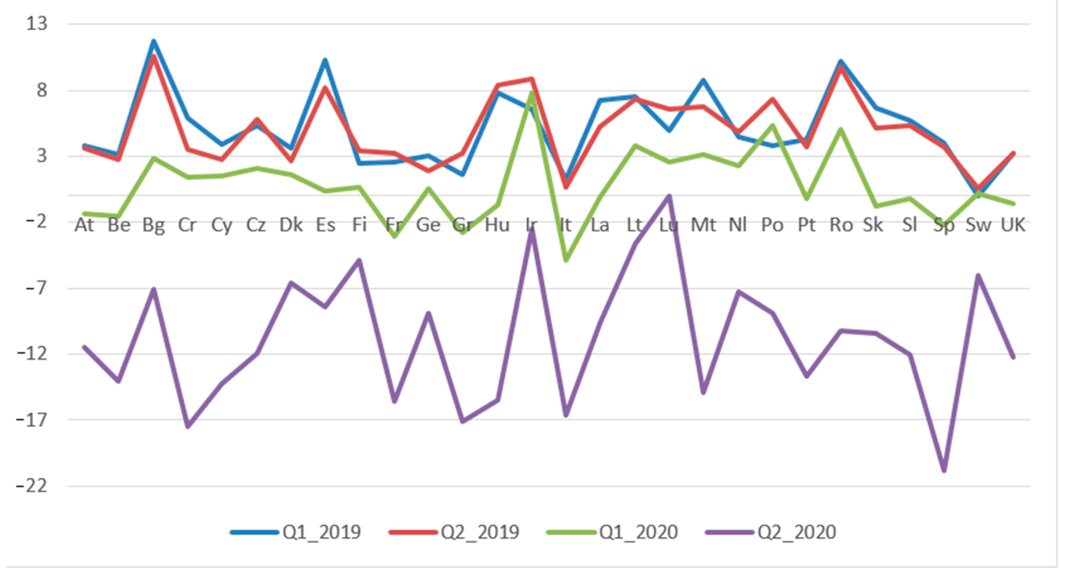
There is a significant reduction in the 2019 growth rate (1.36%) compared to 1996 and obviously there will be a significant decrease in 2020 due to the COVID-19 crisis, which has severely affected the economic growth of all countries. Thus, following the analysis of the first two quarters of 2020 compared to the same period of 2019 (Figure 3), it is observed that the year 2020 began with a relatively slow decline and then intensified in the second quarter, in all EU countries. At EU level (excluding the UK as it left the EU on 1 January 2020) in the first quarter of 2020, the decline in GDP was 4.4%, and in the second quarter compared to the same quarter of 2019 it was 16.65%.

At individual EU states level, in the first quarter of 2020, there is a slight increase compared to the same period of 2019 in most states (16 states). In the second quarter there is a drastic decrease in all EU states, the largest decrease recorded for Spain (20.81%), followed by Croatia and Greece, with over 17%.

For the 1996–2019 time interval, the average calculated at EU level (until 2020) identifies a level of economic growth of 1.53% per year. The homogeneity coefficient exceeds the value of one, revealing a completely heterogeneous structure, asymmetrical to the right, and strongly leptokurtic, with several values concentrated around the average, and high probabilities for extreme values. There is the same trend in all states, respectively, a strong heterogeneity, asymmetric to the right, and leptokurtic (see Appendix A Table A1).

In 2008, compared to 1996, GDP growth rate shows the relative heterogeneity in SL and heterogeneity for the other countries. Twenty-four states have a slight asymmetry, more pronounced to the right for Bg and UK, and two states have a slight asymmetry on the left (Ge and Sl). The distribution is leptokurtic for three states (Bg, Ir, UK), presenting higher probabilities for the extreme values, while for the other states the distribution is platykurtic, with values dispersed in a larger interval around the average (see Appendix A, Table A1).

Compared to 2009, in 2019 GDP growth rate shows heterogeneity for all 28 EU member states. Twenty-three states have a slight asymmetry, while other five have a more pronounced asymmetry, to the right (Dk, Es, Lt, UK) or to the left (Ir). The distribution is leptokurtic for 17 states (At, Be, Cz, Dk, Es, Fi, Fr, Ge, Hu, Ir, La, Lt, Lu, Nl, Sk, Sl, UK) with higher probabilities for extreme values, while for the other states the distribution is platykurtic, with values dispersed in a larger range around the average (see Appendix A, Table A1).

In order to assess living standards in the EU countries, we analyzed GDP per capita, thus eliminating the influence of the absolute size of the population. Following the analysis of the evolution of the GDP per capita for the period 1996–2019, for the EU-28 states, we found a significant increase of this indicator at the level of all states (

Table 1. Analysis of the evolution of gross domestic product per capita (GDP_C) for three time intervals.

Country	GDP_C
	2008/2007 (%)	2008/1996 (%)	Mean (Dollars)	2019/2009 (%)	Mean (Dollars)	2019/1996 (%)	Mean (Dollars)
	1996–2008			2009–2020		1996–2019
At	4.89	68.52	31,821.98	44.32	49,432.56	141.10	39,893.49
Be	3.08	66.86	29,929.16	44.35	45,620.79	140.24	37,121.16
Bg	12.01	109.69	8627.98	73.11	18,350.36	259.26	13,084.07
Cr	7.35	139.34	13,352.57	49.76	23,440.08	245.29	17,976.01
Cy	6.04	101.46	24,369.50	21.63	34,436.30	138.62	28,983.45
Cz	6.59	91.03	19,338.03	54.15	33,356.79	192.09	25,763.29
Dk	5.94	74.18	31,171.11	48.20	49,125.49	152.46	39,400.20
Es	2.98	232.27	13,208.23	88.28	29,071.64	464.86	20,478.96
Fi	6.04	99.90	29,071.66	35.03	43,422.65	155.95	35,649.20
Fr	2.96	64.61	27,894.96	42.42	40,915.82	131.87	33,862.86
Ge	4.28	57.28	29,703.88	52.10	46,864.16	133.21	37,569.01
Gr	5.35	91.40	22,801.42	3.33	28,044.42	94.77	25,204.46
Hu	8.68	121.70	14,374.89	64.20	26,170.92	263.97	19,781.40
Ir	−5.29	116.35	34,128.48	111.85	60,624.03	331.10	46,272.27
It	4.16	54.33	28,633.88	27.60	38,276.53	92.01	33,053.43
La	7.39	237.02	11,088.51	90.14	24,066.24	457.56	17,036.63
Lt	8.64	225.34	11,798.49	110.43	28,012.31	499.33	19,229.82
Lu	3.24	109.80	60,779.36	47.31	101,257.80	193.53	79,331.98
Mt	5.23	91.64	19,738.88	74.51	34,729.51	234.00	26,609.58
Nl	5.76	89.69	34,290.34	33.83	50,654.99	143.90	41,790.81
Po	9.08	121.93	12,302.60	77.65	26,244.11	314.74	18,692.46
Pt	3.73	79.03	20,453.39	37.71	29,892.86	144.85	24,779.81
Ro	22.62	192.61	8470.69	94.00	22,307.89	463.14	14,812.74
Sk	11.91	152.65	14,440.74	47.94	28,677.47	263.96	20,965.91
Sl	7.49	107.27	20,801.74	47.50	32,344.49	184.66	26,092.16
Sp	2.55	96.25	24,458.26	31.41	35,258.38	149.06	29,408.32
Sw	3.17	76.46	31,777.08	38.43	47,995.48	133.62	39,210.51
UK	2.99	67.85	29,083.06	39.05	41,493.60	123.02	34,771.23

).

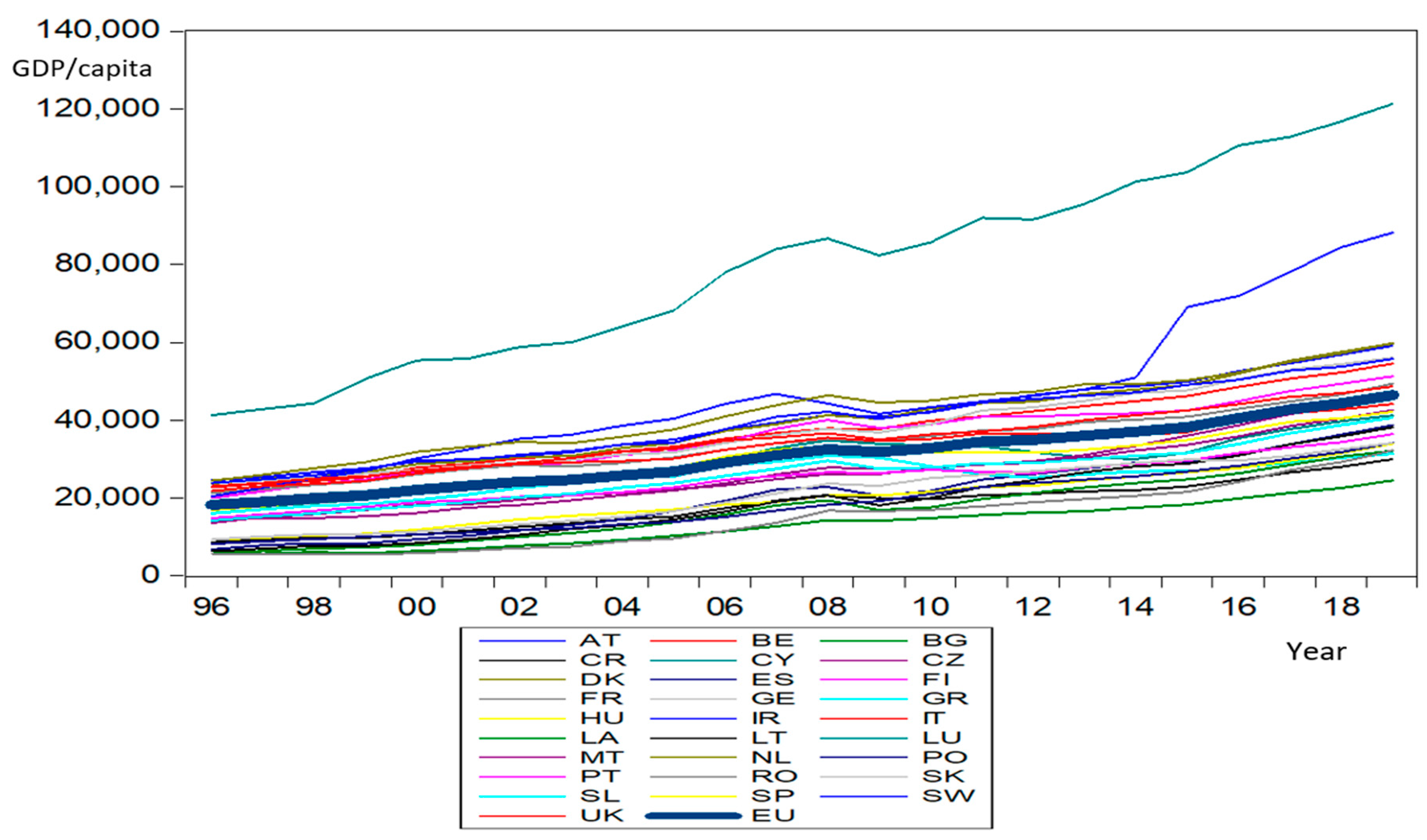
The most significant increases in GDP per capita are noticeable in the emerging states of Estonia, Latvia, Lithuania, and Romania (over 460%), and the smallest increases were in Italy and Greece (Figure 4).

In 2008, the first year of the economic crisis, compared to 2007, GDP per capita increased in almost all states (except for Ir, which fell by 5.09%), although in a much lower percentage than in previous years. The value of GDP_C increased throughout the analyzed period (1996–2019). The largest increase is recorded for all states after the economic crisis (2009–2019). The evolution of the average GDP_C during 1996–2019 is represented in Figure 5.

The average of GDP_C in EU is 30,712.38 dollars/capita. Regarding the distribution of states compared to the EU GDP_C average, it is found that 12 countries have an average greater than the EU average, Luxembourg having an average of two times higher than the EU average, followed by Ireland, the Netherlands, Austria, Denmark, Sweden, Germany, Belgium, Finland, England, France, and Italy. Most member states that joined the EU in 2004, 2007, or 2013 are still far from the EU-28 average. The lowest values of the average GDP_C compared to the EU are Bulgaria (13,084.07 dollars/capita) and Romania (14,812.74 dollars/capita).

The homogeneity coefficient has a value that reveals a relatively heterogeneous structure of GDP_C values for both the EU and most member states (14 states). For Italy and Greece, the value of the homogeneity coefficient shows us that they have a relatively homogeneous structure and for the others the homogeneity coefficient shows a heterogeneous structure. All states have a platikurtic distribution with values scattered over a larger range around the average, most with an asymmetry to the left (22 and EU) or to the right (Cy, Fi, Gr, Nl, Sl, Sp).

In 2008 compared to 1996, GDP_C shows relative homogeneity for At, Be, Dk, Fr, Ge, It, Mt, Nl, Pt, Sw, and UK; relative heterogeneity for Bg, Cr, Cy, Cz, Fi, Gr, Hu, Ir, Lu, Po, Sk, Sl, and Sp; and heterogeneity for other countries. One state has a slight right asymmetry (Ir), and the other ones have a slight left asymmetry. The distribution is platykurtic, with values scattered in a larger range around the average for all 28 EU member states.

In 2019 compared to 2009, GDP_C shows homogeneity for Fi, Gr, It, and Nl; relative homogeneity for At, Be, Bg, Cr, Cy, Cz, Dk, Es, Fr, Ge, Hu, Lu, Mt, Po, Pt, Sk, Sl, Sp, Sw, and UK; and relative heterogeneity for Ir, La, Lt, Ro. One state has a slight right asymmetry (Ge), while the other states have a slight asymmetry to the left. The distribution is platykurtic, with values scattered in a larger range around the average for all 28 EU member states.

Analyzing GDP/capita in the first two quarters of 2020, we find that in the first quarter, at EU-27 level, this indicator decreased by 0.80% compared to 2019, and in the second quarter by 12.39 compared to the same period of 2019. At state level, there is a sharp decrease in the second quarter for all states, with the largest decrease in Spain (21.31%) and the least decrease in Ireland and Lithuania at around 3% (

Table 2. GDP_C evolution for the first two quarters of 2020 compared to the same period of 2019.

Country	2019Q1 (Dollars)	2019Q2 (Dollars)	2020Q1 (Dollars)	2020Q2 (Dollars)	20/19Q1 (%)	20/19Q2 (%)
At	10,960.00	11,090.00	10,770.00	9770.00	−1.73	−11.90
Be	9910.00	10,390.00	9710.00	8890.00	−2.02	−14.44
Bg	1820.00	2150.00	1880.00	2020.00	3.30	−6.05
Cr	2910.00	3330.00	2970.00	2770.00	2.06	−16.82
Cy	5890.00	6370.00	5920.00	5400.00	0.51	−15.23
Cz	4850.00	5260.00	4940.00	4610.00	1.86	−12.36
Dk	12,820.00	13,460.00	12,990.00	12,550.00	1.33	−6.76
Es	4910.00	5310.00	4920.00	4850.00	0.20	−8.66
Fi	10,370.00	11,040.00	10,410.00	10,480.00	0.39	−5.07
Fr	8870.00	9000.00	8580.00	7580.00	−3.27	−15.78
Ge	10,190.00	10,200.00	10,230.00	9280.00	0.39	−9.02
Gr	3970.00	4460.00	3870.00	3700.00	−2.52	−17.04
Hu	3290.00	3670.00	3260.00	3100.00	−0.91	−15.53
Ir	17,320.00	17,260.00	18,450.00	16,630.00	6.52	−3.65
It	7060.00	7350.00	6740.00	6160.00	−4.53	−16.19
La	3530.00	4000.00	3540.00	3630.00	0.28	−9.25
Lt	3840.00	4320.00	3980.00	4160.00	3.65	−3.70
Lu	24,460.00	25,540.00	24,620.00		0.65
Mt	6300.00	6610.00	6250.00	5480.00	−0.79	−17.10
Nl	11,370.00	11,920.00	11,540.00	10,990.00	1.50	−7.80
Po	3160.00	3330.00	3330.00	3040.00	5.38	−8.71
Pt	4920.00	5160.00	4900.00	4440.00	−0.41	−13.95
Ro	2210.00	2660.00	2320.00	2390.00	4.98	−10.15
Sk	3970.00	4340.00	3940.00	3880.00	−0.76	−10.60
Sl	5360.00	5810.00	5310.00	5080.00	−0.93	−12.56
Sp	6350.00	6710.00	6160.00	5280.00	−2.99	−21.31
Sw	11,330.00	11,840.00	11,240.00	11,040.00	−0.79	−6.76
UK	7490.00	7750.00	7430.00	6790.00	−0.80	−12.39

).

Another indicator of appreciation of the level of economic development is the employed population. The labor force participation rate at EU level in 2019 was above the value in 1996, increasing by 3.92%, but at states level the situation is very different, with the evolution of this indicator varying between countries (

Table 3. Labor evolution analysis for three time intervals.

Country	Labor
	2008/2007 (%)	2008/1996 (%)	Mean (%)	2019/2009 (%)	Mean (%)	2019/1996 (%)	Mean (%)
	1996–2008			2009–2019		1996–2019
At	0.4	2.28	58.9	1.52	60.87	4.31	59.78
Be	0.16	6.49	52.38	1.72	53.63	7.9	52.71
Bg	2.3	3.88	51.14	6.71	54.06	9.24	52.7
Cr	0.36	36.55	50.88	−3.79	51.82	31.37	50.8
Cy	−0.46	−4.47	59.25	2.9	59.37	4.45	62.91
Cz	−0.46	−4.47	59.25	2.9	59.37	−1.41	59.56
Dk	−0.96	−0.17	65.57	−3.14	62.25	−4.33	64.02
Es	0.91	−5.6	59.27	4.83	62.03	−1.67	61.01
Fi	0.4	3.57	62.13	−1.76	59.41	0.11	60.64
Fr	0.16	1.07	56.07	−2.21	56.08	−0.79	56
Ge	0.15	2.82	58.02	4.25	60.48	7.47	59.09
Gr	0.08	6.67	52.53	−2.79	52.35	4.62	52.15
Hu	−0.82	3.3	49.74	14.53	53.54	18.18	51.26
Ir	−1.03	20.18	61.69	−2.72	62.23	13.61	61.02
It	0.72	3.49	48.91	2.92	49.08	5.16	48.79
La	2.14	2.99	58.17	1.83	60	2.46	59.16
Lt	0.49	−8.8	57.56	9.79	59.01	1.45	58.72
Lu	0.14	9.91	54.85	4.27	59.13	19.01	56.25
Mt	0.39	4.3	49.76	22.44	55.12	28.18	51.51
Nl	1.18	9.37	64.34	−1.01	64.61	8.49	63.94
Po	0.96	−6.86	55.02	2.32	55.93	−3.46	55.82
Pt	−0.29	7.47	61.78	−3.42	59.61	2.66	60.35
Ro	−0.48	−15.88	57.24	1.28	54.61	−14.91	57.37
Sk	0.77	−1.4	59.66	1.4	59.42	−0.75	59.54
Sl	−0.35	3.44	58.48	−2.3	58.02	0.97	58.24
Sp	1.35	17.9	55.82	−2.65	58.92	15.02	56.43
Sw	0.39	4.28	62.77	15.87	71.14	19.65	66.28
UK	0.38	1.74	62.14	1.05	62.72	2.48	62.34

).

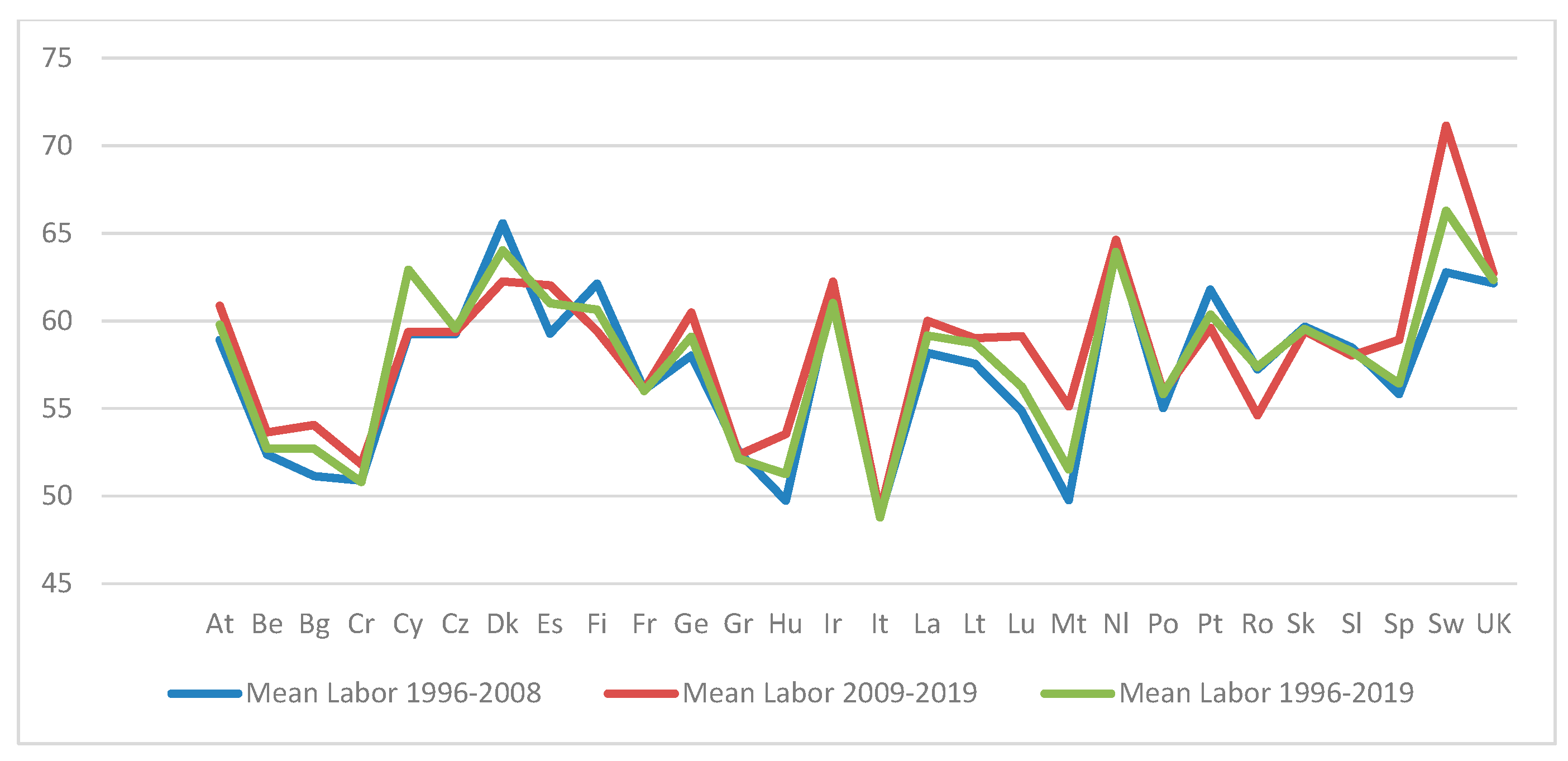
Analyzing Labor by periods, there is a decrease in the labor force in 2009 compared to 2008 in eight states (Cy, Cz, Dk, Hu, Ir, Pt, Ro, Sl), but the mean value in the following period shows an increase in population occupied in most states (Figure 6). For the economically developed states, however, we find a decrease in Labor throughout the period 1996–2019; this decrease is accentuated in the period following the 2009–2019 crisis.

Italy has the lowest employment rate at around 49%, followed by Croatia at around 50%. The highest averages are recorded by economically developed countries (Sw, UK, Nl, Dk, Ir, Pt), mainly due to the attraction of labor force from emerging EU countries.

Fifteen countries have a labor force participation rate higher than EU; the highest increases in 2019 compared to 1996 are recorded in Croatia (31.37%) and Malta (28.18%), and the lowest increase is recorded in Finland (0.11%). It should be noted that in seven countries (Sk, Fr, Cz, Es, Po, Dk, Ro) the labor force participation rate decreased, and the most significant decrease was in Romania with a percentage of 14.9% (Figure 7).

The continuous increase in labor force participation rates in the EU contrasted with a decrease in population of 1.3%.

For the 1996–2019 interval, the statistical analysis of the indicator shows a homogeneous distribution of the labor force participation rate over the studied period; the indicator does not show extreme variations either at the EU level or at individual level.

The average labor force participation rate also shows that most countries (18) have a higher average than the EU average; Sweden has the highest value (66.28%) and Italy has the lowest value (48.79%). In 2019, the trend is largely maintained; the labor force participation rate at EU level was 57.58%, with Sweden having the highest labor force participation rate (73.36%) and Italy the lowest (49.89%).

Greece, the Netherlands, and Malta have a leptokurtic distribution, sharper than the normal distribution, with more values concentrated around the average and showing extreme values. The other countries have a platikurtic distribution, with homogeneously dispersed values around the average. Bulgaria, Czechia, Estonia, Finland, Germany, Hungary, Romania, and Slovakia show a slight asymmetry to the left, and the others a slight asymmetry to the right.

In 2008 compared to 1996, labor force participation rates are homogeneous for all 28 EU member states. Sixteen states have a slight asymmetry to the right (At, Be, Dk, Fi, Fr, Gr, Hu, It, Lu, Mt, Nl, Pt, Sk, Sl, Sp, Sw), while the other states have a slight asymmetry to the left. The distribution is leptokurtic for one state (Sw), presenting higher probabilities for the extreme values, while for the other states the distribution is platykurtic, with values dispersed in a larger interval around the average.

For 2019 compared to 2009, labor force participation rates show homogeneity in all 28 EU member states. Eight states have a slight (Fr, Hu, It, Lu, Po, Ro, Sk, Sp) or a more pronounced (Sw) asymmetry to the right, while the other states have a slight asymmetry to the left, except for Ir where the left asymmetry is more pronounced. The distribution is leptokurtic for two states (Ir and Sw) presenting higher probabilities for the extreme values, and for the other states the distribution is platykurtic, with values dispersed in a larger interval around the average.

Regarding 2020 (Figure 8), the effect of the COVID-19 pandemic on the labor force participation rate is imperceptible in the first quarter; however, the decrease in the rate is evident for the second quarter in almost all states (except Croatia), the largest decrease recorded by Spain (almost 7%).

The main factor of economic growth along with the final consumption by the population is the gross fixed capital formation. Across the EU, GCF growth was only 1.3% in 2019 compared to 1996; this was due to the fact that in a number of important countries the value of investments in GDP remained at about the same value or even decreased when compared to 1996.

Greece had the largest decrease in GCF (45%), followed by Sk (34%) and Cz, Pt, Cy, and Mt with over 20%. In contrast, the highest increases were registered by Bulgaria with 310% and Ireland with 119.4%, which, however, also had very strong variations (

Table 4. Analysis of the evolution of the share of investments in GDP.

Country	GCF
	2008/2007 (%)	2008/1996 (%)	Mean (%)	2019/2009 (%)	Mean (%)	2019/1996 (%)	Mean (%)
	1996–2008			2009–2020		1996–2019
At	1.57	−9.75	24.24	8.37	22.94	−5.83	23.65
Be	3.54	13.85	22.03	5.84	23.01	13.84	22.48
Bg	16.60	641.33	19.63	−34.32	20.86	310.00	20.19
Cr	5.31	53.10	23.35	−18.04	20.51	12.31	22.05
Cy	6.40	12.94	22.30	−18.58	17.92	−20.71	20.30
Cz	−1.80	−14.61	29.81	−5.85	25.80	−24.89	27.97
Dk	−2.42	17.03	21.43	10.02	19.97	13.19	20.76
Es	−14.58	14.89	30.71	15.71	24.91	−3.58	28.05
Fi	1.23	19.47	22.50	3.10	22.65	15.43	22.57
Fr	1.78	18.81	21.35	7.06	22.30	18.96	21.78
Ge	1.23	−11.83	21.11	12.78	20.29	−5.63	20.73
Gr	−8.45	14.53	23.56	−45.08	13.54	−45.08	18.97
Hu	−1.51	2.17	24.05	26.03	22.06	25.03	23.14
Ir	−13.63	25.17	25.01	105.97	24.72	119.44	24.88
It	−1.77	10.84	20.63	−10.23	18.14	−5.96	19.49
La	−11.94	79.59	26.62	2.24	22.02	28.15	24.51
Lt	−8.88	26.54	22.88	18.27	19.01	2.66	21.11
Lu	10.05	2.15	20.31	−8.29	18.51	−14.92	19.49
Mt	−12.26	−20.11	21.85	7.97	19.81	−20.21	20.92
Nl	−5.05	2.53	21.66	−1.38	19.95	−2.59	20.87
Po	−5.05	2.53	21.66	−1.38	19.95	−4.20	20.29
Pt	1.52	−4.08	24.94	−13.51	17.23	−23.03	21.40
Ro	5.50	62.80	23.91	−9.09	24.59	3.19	24.22
Sk	−2.66	−25.07	28.34	3.50	21.35	−34.83	25.14
Sl	2.76	23.36	26.51	−20.01	19.61	−19.12	23.35
Sp	−6.78	28.36	26.26	−13.40	19.33	−7.71	23.09
Sw	1.57	21.32	22.12	8.65	23.55	20.80	22.77
UK	−3.36	−6.11	17.66	7.17	16.37	−8.21	17.07

).

Analyzing GCF in the first year after the crisis, it is observed that in most states the value of investments decreased. The emerging states had higher increases (Bg 16.6% and Ro 5.5%) than the developed states (between 1–3%). After the crisis period (2009–2019), there is a moderate increase in investment in 16 states (At, Be, Cz, Dk, Es, Fi, Fr, Ge, Hu, Ir, La, Lt, Mt, Sk, Sw, UK), the highest increase in Ireland (105.97%) and the lowest La and Fi, around 3%. The other states registered decreases, the largest decrease registered by Greece with 45.08%.

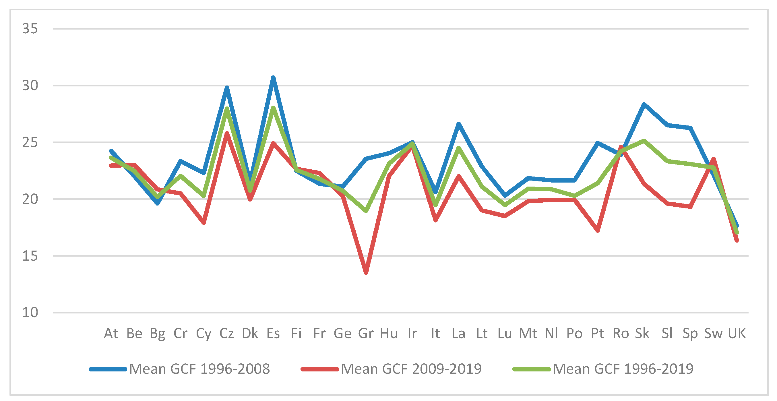
The largest investments are obviously made until the crisis, averaging around 20% of GDP (excluding the UK, 17.66%). The average values for the period 1996–2019 are lower than those for the period 1996–2008, which means that gross fixed capital formation in the EU-28 has not fully recovered since its dramatic collapse in 2009, although it has shown relative increases each year (Figure 9).

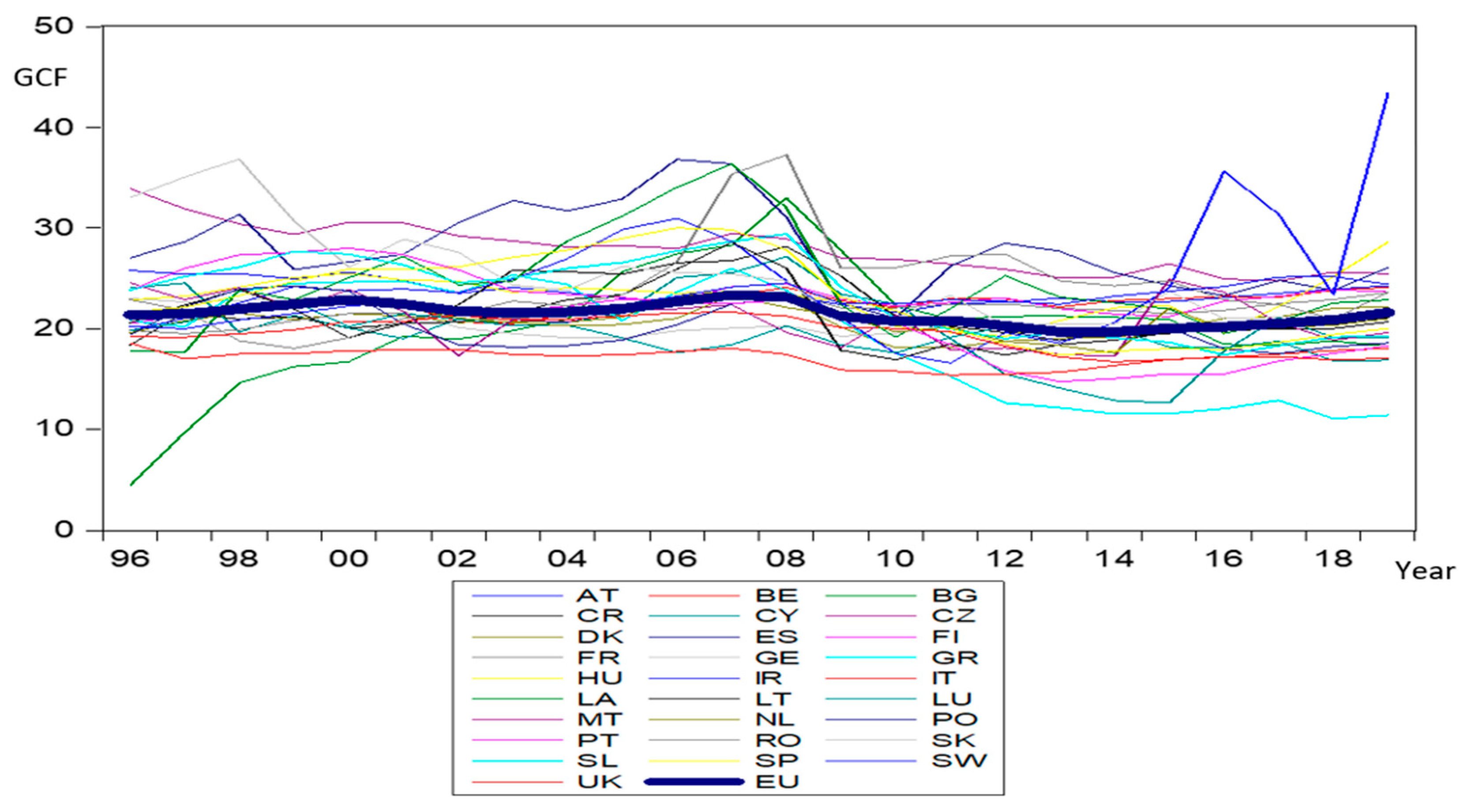
Thus, it is observed that at the level of EU member states (Figure 10), there are large differences in terms of investment intensity, which is reflected, in part, in the different stages of economic development of countries, as well as the dynamics of growth in later years. The average of GCF at EU level for the period 1996–2019 is 21.44%; 15 states have higher average values than the EU average, the highest averages registered by Estonia (28.05%) and Czechia (27.99%).

In 2019, gross fixed capital formation (in current prices) as a percentage of GDP was 21.64% at EU-28 level, with 13 countries having higher GCF shares than the EU average, with the highest values in Ireland (43.4%), followed by Hungary (28.6%), Estonia and Czechia (over 25%), and the other 15 countries registering values lower than the EU average, with the lowest level in Greece (11.42%).

In 2019 compared to 1996, according to the analysis of the homogeneity coefficient, it is observed that 13 states and the EU as a whole have a homogeneous structure of GCF values, 11 countries have a relatively homogeneous GCF value, and the other four states (Croatia, Cyprus, Estonia, and Portugal) have relatively heterogeneous values.

GCF for most EU member states and the EU as a whole has a platikurtic distribution, with the exception of Bulgaria, Hungary, Ireland, Latvia, Lithuania, and Romania, which have a leptokurtic distribution. Half of the countries and the EU have a slight asymmetry to the left, and the other 14 states have a slight asymmetry to the right.

For 2008 compared to 1996, GCF shows homogeneity (for At, Be, Cz, Dk, Fi, Fr, Ge, Gr, Hu, It, Lu, Mt, Nl, Po, Pt, Sl, Sw, UK), relative homogeneity (for Cr, Cy, Es, Ir, Lt), and relative heterogeneity (La, Sk, Sp) or heterogeneity (Bg and Ro). Six states have a slight asymmetry to the right (Bg, Gr, It, Lu, Mt, Sp), while the others have a slight asymmetry to the left. The distribution is platykurtic, with values scattered in a larger range around the average for all 28 EU member states.

In 2019 compared to 2009, GCF shows homogeneity (in At, Be, Cr, Cz, Dk, Es, Fi, Fr, Ge, It, La, Lt, Lu, Nl, Po, Ro, Sk, Sl, Sp, Sw, UK), relative homogeneity (in Bg, Hu, Mt, Pt), or relative heterogeneity (Cy, Gr, Ir). Ten states have a slight asymmetry to the right (Cy, Es, Fi, La, Lt, Lu, Nl, Po, Ro, UK), while the other states have a slight asymmetry to the left, except for Cr where it is more pronounced. The distribution is leptokurtic for three states (Bg, Cr, Sl), presenting higher probabilities for the extreme values, while for the others the distribution is platykurtic, with values dispersed in a larger interval around the average.

At EU-27 level, the first quarter of 2020 marked an increase in the share of GCF in GDP of 3.4% (

Table 5. Evolution of GCF in the first two quarters of 2019 and 2020.

Country	2019Q1 (%)	2019Q2 (%)	2020Q1 (%)	2020Q2 (%)	20/19Q1 (%)	20/19Q2 (%)
At	22.5	24.5	22.7	25.0	0.888889	2.040816
Be	23.5	23.6	23.2	21.7	−1.2766	−8.05085
Bg	15.3	19.7	13.9	18.9	−9.15033	−4.06091
Cr	22.2	21.7	22.6	22.4	1.801802	3.225806
Cy	16.1	20.6	21.0	12.4	30.43478	−39.8058
Cz	23.9	24.5	23.2	25.6	−2.92887	4.489796
Dk	22.2	22.2	21.9	22.4	−1.35135	0.900901
Es	25.2	27.9	23.1	25.0	−8.33333	−10.3943
Fi	22.3	24.3	22.3	25.5	0	4.938272
Fr	23.1	23.6	22.7	22.3	−1.7316	−5.50847
Ge	20.2	22.3	20.6	23.0	1.980198	3.139013
Gr	11.0	11.7	10.6	12.6	−3.63636	7.692308
Hu	21.8	29.7	21.5	29.8	−1.37615	0.3367
Ir	20.9	71.7	51.2	20.8	144.9761	−70.9902
It	18.7	18.9	17.9	17.7	−4.27807	−6.34921
La	18.9	21.4	20.4	22.6	7.936508	5.607477
Lt	19.2	21.5	19.3	19.9	0.520833	−7.44186
Lu	17.0	17.1	14.8		−12.9412	−
Mt	24.9	20.7	21.1	21.9	−15.261	5.797101
Nl	21.4	21.7	22.3	21.5	4.205607	−0.92166
Po	13.3	16.8	13.0	16.0	−2.25564	−4.7619
Pt	18.5	18.5	18.9	19.9	2.162162	7.567568
Ro	15.5	23.5	17.0	26.5	9.677419	12.76596
Sk	18.8	20.1	18.1	19.3	−3.7234	−3.9801
Sl	19.5	19.9	18.9	19.0	−3.07692	−4.52261
Sp	20.5	20.2	20.1	19.3	−1.95122	−4.45545
Sw	23.7	25.1	23.7	25.4	0	1.195219
UK	17.6	16.5	17.3	14.3	−1.70455	−13.3333
EU-27	20.6	23.0	21.3	21.5	3.398058	−6.52174

). Regarding the share of investments in GDP by state, in the first quarter of 2020 compared to 2019 there is a decrease in most states (except for Ro, Po, Nl, La, Lt, Ge, Cy, Cr, At), the largest decrease being registered by Luxembourg (12.94%). In the second quarter compared to the same period of 2019, 11 countries mark an increase in GCF in GDP, but for EU-27 there is a decrease of 6.5%. The largest decrease is recorded by Ireland (71%).

Given that remittances represent a capital inflow into the country of origin, remittances can affect the country’s economic balance and the macroeconomic variable GDP. Remittances are an important source of foreign transfers to developing countries and can be considered a financial mechanism for development. The trend of this currency inflow in the countries of origin obviously illustrates that the value of remittances decreases visibly [8,55], and the strategic analysis of this trend, especially due to the COVID-19 pandemic cannot be optimistic—foreign exchange inflows into countries of origin will fall drastically. The economic and geopolitical situation of the host countries is only one of these factors, but the UK’s exit from the EU (1 January 2020) will clearly have a negative impact on remittance inflows to the external balance of payments of emerging countries.

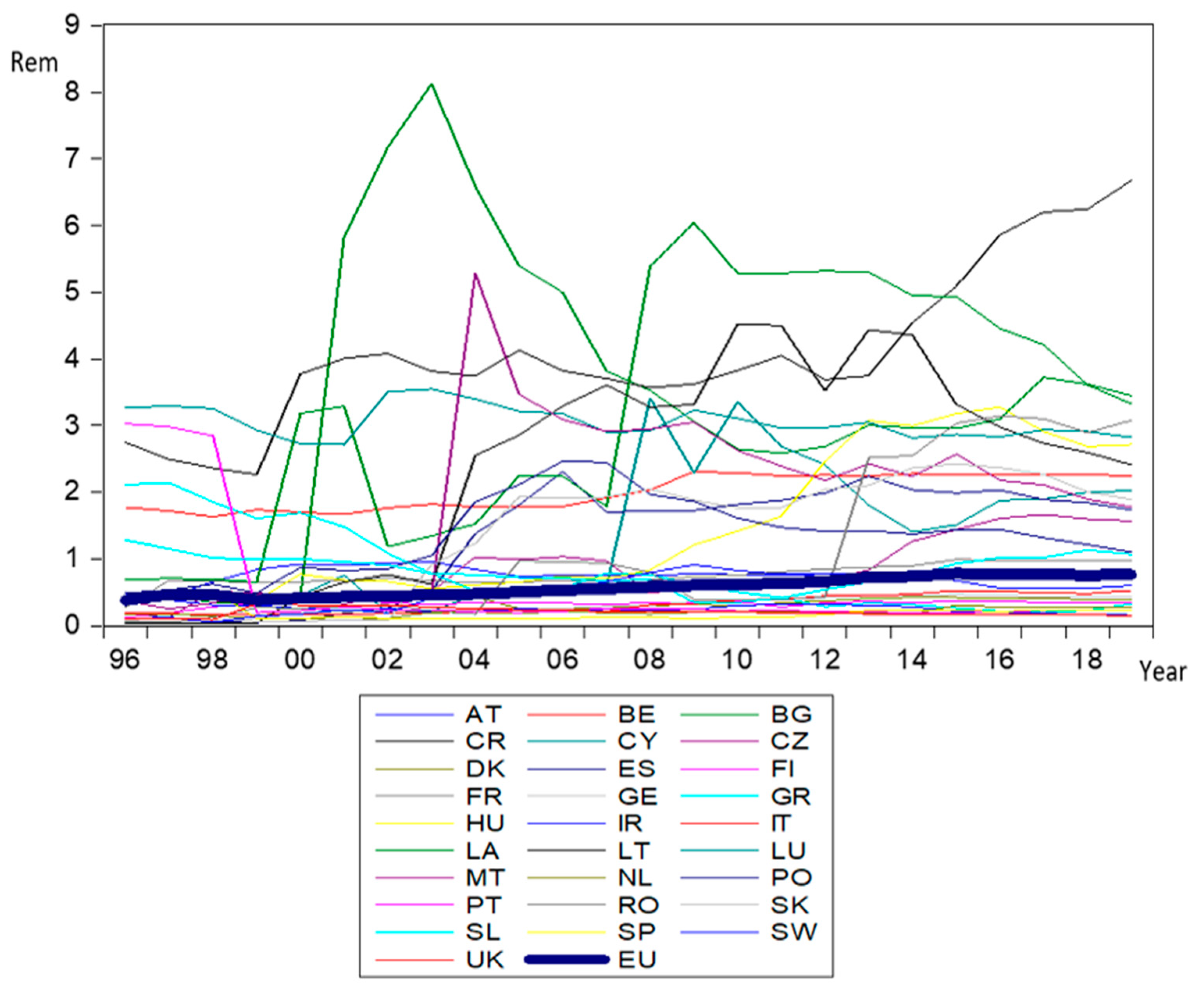
The share of remittances in GDP represents an increase of 100.58% in 2019 compared to 1996. The largest increases in Rem_GDP were, as expected, in the emerging countries Lt, Ro, Sk, Es, Cz, Bg, Hu, with the share of remittances in GDP increasing from around 0.03% to over 3% (

Table 6. Evolution of the share of Remittances in GDP.

Country	Rem_GDP
	2008/2007 (%)	2008/1996 (%)	Mean (%)	2019/2009 (%)	Mean (%)	2019/1996 (%)	Mean (%)
	1996–2008			2009–2020		1996–2019
At	−1.17	78.68	0.76	−10.96	0.74	66.35	0.75
Be	6.38	14.79	1.78	−3.13	2.26	25.96	2.00
Bg	−7.59	944.09	3.64	12.63	3.07	921.45	3.38
Cr	−3.76	30.03	3.42	84.36	4.87	143.51	4.08
Cy	474.34	591.54	0.70	−11.58	2.11	310.51	1.35
Cz	−50.15	191.82	0.58	169.90	1.13	849.37	0.83
Dk	15.49	−18.79	0.38	21.51	0.37	5.17	0.38
Es	0.56	4747.81	0.77	0.46	1.92	4810.14	1.30
Fi	7.09	206.19	0.31	−2.20	0.34	204.61	0.32
Fr	3.99	154.93	0.63	33.18	0.89	260.59	0.75
Ge	3.05	69.71	0.22	17.91	0.42	147.12	0.31
Gr	−2.78	−64.09	1.22	−47.40	0.33	−84.73	0.81
Hu	19.00	148.38	0.59	125.25	2.50	712.20	1.47
Ir	5.46	−51.78	0.27	−37.78	0.24	−68.40	0.26
It	47.47	59.27	0.19	62.63	0.45	171.47	0.31
La	202.29	686.24	1.91	−45.02	4.79	385.13	3.23
Lt	−9.29	10,552.33	1.40	−27.38	3.51	7731.32	2.37
Lu	0.85	−10.56	3.14	−12.63	2.95	−13.55	3.05
Mt	1.25	701.57	1.60	−41.72	2.31	383.28	1.93
Nl	−9.57	12.41	0.16	33.56	0.23	70.32	0.19
Po	−19.57	305.50	1.27	−40.97	1.42	126.72	1.34
Pt	−3.80	−91.92	0.86	−6.61	0.21	−92.42	0.56
Ro	−14.62	1529.99	0.41	684.72	1.99	6212.15	1.14
Sk	6.19	2641.52	0.80	0.49	2.08	2435.32	1.39
Sl	2.62	−46.55	0.89	209.25	0.74	−16.83	0.82
Sp	−0.56	−75.12	0.19	123.38	0.19	−49.64	0.19
Sw	21.24	755.04	0.33	−34.08	0.71	547.59	0.50
UK	−2.98	104.25	0.22	−32.84	0.18	45.43	0.20

, Figure 11). A decrease in Rem_GDP was recorded in six countries (Gr, Ir, Lu, Pt, Sl, Sp) with the largest decrease recorded in Portugal (92.42%) and followed by Greece (84.73%).

The share of remittances in GDP has increased significantly in emerging countries due to the free movement of people in the EU, which has led to an increase in labor migration to developed countries.

In the pre-crisis period, developed countries received massive labor from emerging countries, which led to an increase in the value of remittances sent to their countries of origin, the largest increase recorded by Lithuania, followed by Estonia. In the post-crisis period, their share in GDP decreased but remained significant.

The analysis of the average share of remittances in GDP shows a significant increase after the crisis (2009–2019) (Figure 12); most states recorded increases of average Rem_GDP, except for Pt and Gr, which recorded significant decreases. UK, Sp, Ir, and Dk generally remained at the same values.

In 2019 compared to 1996, the share of remittances in GDP shows homogeneity in Luxembourg, relative homogeneity in four states (At, Be, Dk, Fi), relative heterogeneity for four states (Cr, Fi, Ir, Nl), and heterogeneity for the other states. Ten states have a slight asymmetry and Finland a more pronounced asymmetry to the right, and the other states generally have a slight left asymmetry (except Pt). The distribution is leptokurtic for six states (At, Fi, Fr, Ir, Pt, Sp) presenting higher probabilities for the extreme values, and for the other states the distribution is platikurtic, with values dispersed over a larger range around the average.

In 2008 compared to 1996, Rem_GDP shows homogeneity (in Be, Lu), relative homogeneity (in Cr, Fr, Ge), relative heterogeneity (in At, Dk, Fi, Hu, Ir, It, Nl, Sl), and heterogeneity for the other countries. Seven states have a slight (As, Cr, Dk, Fi, Hu, Lu, NL) or more pronounced (Fr) asymmetry to the right, while the other states have a slight asymmetry on the left, except Cy where it is more pronounced. The distribution is leptokurtic for six states (Cy, Fi, Fr, Ir, It, La) presenting higher probabilities for the extreme values, while for the others the distribution is platykurtic, with values dispersed in a larger interval around the average.

In 2019 compared to 2009, Rem_GDP shows homogeneity (in At, Be, Es, Fi, Ge, Lu, Pt), relative homogeneity (in Bg, Dk, Fr, It, La, Mt, Nl, Po, Sk, Sw), relative heterogeneity (in Cr, Cy, Hu, Ir, Lt, Sp), and heterogeneity for the other countries. Thirteen states have a slight (At, Cz, Dk, Fr, Ge, Hu, Ir, It, La, Pt, Ro, Sl, Sp) or more pronounced (Fi) asymmetry to the right, while the other states have a slight asymmetry to the left. The distribution is leptokurtic for one state (Fi) presenting higher probabilities for the extreme values, while for the others the distribution is platykurtic, with values dispersed in a larger interval around the average.

3.2. Analysis of the Stationary Value of the Indicators

For stationarity analysis of indicators, we started from Model (1) and verified the stationarity of the data series using the Dickey–Fuller test, the option with individual effects and the automatic lag selection. The results of the unit root test, LLC (Levin-Lin-Chu), performed on each country, show that the null hypothesis, the existence of a common unitary root, cannot be rejected, as these processes are partly nonstationary.

The results of the ADF (Augmented Dickey Fuller) tests for the first difference, performed for the indicators at nominal values, lead to the conclusion that the null hypothesis of the existence of a unit root can be rejected for all countries for the G_GDP variable, where the processes are stationary at a 1% confidence level. Unit root tests for the first difference showed that for the other four indicators, the processes are stationary for most states, the null hypothesis being rejected at a level of confidence differentiated from 1% to 10%.

Since there is a difference between the orders of magnitude, we proceeded to test a model in which we logarithmed the four independent variables, obtaining Equation (2):

$${\mathrm{y}}_{\mathrm{it}}={\mathrm{u}}_{\mathrm{i}}+{ \mathsf{\beta }}_1\log {\mathrm{a}}_{\mathrm{i},\mathrm{t}-1}+{ \mathsf{\beta }}_2{\log \mathrm{b}}_{\mathrm{it}}+{ \mathsf{\beta }}_3\log {\mathrm{c}}_{\mathrm{it}} +{ \mathsf{\beta }}_4\log {\mathrm{a}}_{\mathrm{i},\mathrm{t}-1}+{\mathsf{\epsilon }}_{\mathrm{it}}$$

(4)

We checked the stationarity of the variables in logarithmic form. The results of the ADF–Fisher level tests were not significant. Thus, the first difference was tested, leading to the following conclusions: for GDP_C the null hypothesis of the existence of a unit root can be rejected for most states (except Greece and Spain) at a confidence level differentiated from 1% to 10%; for Labor, variables are stationary in all countries at a confidence level of 1–10%; and for GCF there is no single root in the 1–10% confidence interval. Therefore, processes are stationary for most states (with the exception of Italy, Portugal, Spain, and the EU as a whole). Regarding Rem_GDP, the states with the nonstationary processes are Austria, Estonia, Germany, Greece, and Sweden, otherwise the states are stationary and differentiated between 1–10%.

We then continued to stationary the nonstationary series (GDP_C, Labor, GCF and Rem_GDP), making the difference twice (second order of integration), and the newly generated series were tested again with the augmented Dickey–Fuller statistical test. The results show that for each of the variables tested, t-statistic is less than t-critical and p-value associated less than 5%, so the null hypothesis is rejected and the alternative hypothesis accepted, so the series have no unit roots, thus they are stationary (see Appendix A,

Table A2. Testing the stationarity of the derived variables.

Country	First Differences—Test Critical Values: 1% (−3.788030) 5% (−3.012363) 10% (−2.646119)
	DL_GDP_C		DL_Labor		DL_GCF		DL_Rem_GDP
	t-Stat.	Prob.	t-Stat.	Prob.	t-Stat.	Prob.	t-Stat.	Prob.
At	−5.23157 *	0.0005	−6.21098 *	0.0001	−5.43344 *	0.0004	−4.51174 *	0.0022
Be	−4.52479 *	0.0028	−6.04869 *	0.0001	−6.77716 *	0	−6.60247 *	0
Bg	−13.0078 *	0	−7.98806 *	0	−4.6532 *	0.0015	−4.12389 *	0.0051
Cr	−4.71959 *	0.0013	−3.94772 *	0.0111	−6.0387 *	0.0001	−6.65418 *	0
Cy	−3.60391 **	0.0148	−4.12718 *	0.0073	−6.87884 *	0	−4.96932 *	0.0009
Cz	−5.06237 *	0.0006	−6.92916 *	0	−6.15177 *	0.0001	−11.427 *	0
Dk	−10.2262 *	0	−8.15282 *	0	−4.5243 *	0.002	−9.01332 *	0
Es	−5.63098 *	0.0002	−7.37342 *	0	−4.59661 *	0.0019	−6.6602 *	0
Fi	−5.33226 *	0.0004	−7.29835 *	0	−4.65242 *	0.0018	−4.97383 *	0.0008
Fr	−5.92361 *	0.0001	−5.23835 *	0.0005	−5.0844 *	0.0006	−4.91223 *	0.0011
Ge	−4.50945 *	0.0029	−8.20996 *	0	−4.98001 *	0.0007	−10.7857 *	0
Gr	−6.10365 *	0.0001	−4.54972 *	0.0027	−5.12289 *	0.0006	−4.81419 *	0.0011
Hu	−7.80943 *	0	−6.20902 *	0	−5.19946 *	0.0006	−7.47007 *	0
Ir	−6.95682 *	0	−5.51938 *	0.0002	−5.94541 *	0.0001	−6.06637 *	0.0001
It	−5.3582 *	0.0003	−5.96663 *	0.0001	−5.67702 *	0.0002	−7.9412 *	0
La	−5.29412 *	0.0004	−5.13609 *	0.0007	−4.06015 *	0.0066	−5.45627 *	0.0004
Lt	−5.62371 *	0.0002	−8.52097 *	0	−5.50826 *	0.0003	−13.8515 *	0
Lu	−5.98759 *	0.0001	−5.35354 *	0.0005	−7.26151 *	0	−5.79609 *	0.0002
Mt	−6.50276 *	0	−5.95409 *	0.0001	−4.77079 *	0.0016	−8.71667 *	0
Nl	−6.23105 *	0	−5.54832 *	0.0002	−9.32579 *	0	−6.28837 *	0.0001
Po	−7.13681 *	0	−5.25256 *	0.0005	−3.40075 **	0.0259	−8.65471 *	0
Pt	−6.19839 *	0.0001	−11.2278 *	0	−4.85996 *	0.001	−7.26309 *	0
Ro	−6.83488 *	0	−4.89436 *	0.001	−4.64253 *	0.0018	−7.13544 *	0
Sk	−7.36773 *	0	−8.06949 *	0	−7.39264 *	0	−8.26402 *	0
Sl	−6.74574 *	0	−6.7834 *	0	−5.1859 *	0.0005	−6.62256 *	0
Sp	−4.80854 *	0.0011	−6.34008 *	0	−5.13353 *	0.0005	−7.49612 *	0
Sw	−6.15231 *	0.0001	−8.33274 *	0	−4.65639 *	0.0016	−9.99406 *	0
UK	−8.9603 *	0	−6.64652 *	0	−7.11406 *	0	−8.77448 *	0
UE	−6.20187 *	0.0001	−7.47857 *	0	−4.86103 *	0.0011	−6.0545 *	0.0001

* Denotes significance at 1% level, ** denotes significance at 5% level.

).

Therefore, the multiple linear difference Model (2) is validated, as follows:

$$\mathrm{G}\_{\mathrm{GDP}}_{\mathrm{it}}={\mathrm{C}}_{\mathrm{i}}+{\mathsf{\beta }}_1\mathrm{D} \mathrm{L}\_\mathrm{GDP}\_{\mathrm{C}}_{\mathrm{it}-1}+{ \mathsf{\beta }}_2\mathrm{D} \mathrm{L}\_{\mathrm{Labor}}_{\mathrm{it}}+{ \mathsf{\beta }}_3\mathrm{D} \mathrm{L}\_{\mathrm{GFC}}_{\mathrm{it}} +{ \mathsf{\beta }}_4\mathrm{D} \mathrm{L}\_\mathrm{Rem}\_{\mathrm{GDP}}_{\mathrm{it}-1}+{\mathsf{\epsilon }}_{\mathrm{it}}$$

(5)

To further validate Model (3), we used the Granger causality test. Taking into account Equation (3), only the causality of the variables Labor, GFC, and Rem_GDP toward GDP was reported in

Table 7. Granger causality tests.

Country	GCF-G_GDP		Labor-G_GDP		Rem_GDP-G_GDP
	Probability	Conclusion	Probability	Conclusion	Probability	Conclusion
At	0.0162	Reject	0.1216	Reject	0.2916	Reject
Be	0.0033 *	Accept	0.0891 *	Accept	0.0792 *	Accept
Bg	0.0045 *	Accept	0.2125	Reject	0.0013 *	Accept
Cr	0.0001 *	Accept	0.082 *	Accept	0.0902 *	Accept
Cy	0.0018 *	Accept	0.0263 *	Accept	0.0501 *	Accept
Cz	0.1803	Reject	0.0854 *	Accept	0.1084	Reject
Dk	0.0000 *	Accept	0.0522 *	Accept	0.008 *	Accept
Es	0.0688 *	Accept	0.2101	Reject	0.0257 *	Accept
Fi	0.0055 *	Accept	0.0629 *	Accept	0.0158 *	Accept
Fr	0.0013 *	Accept	0.0724 *	Accept	0.3556	Reject
Ge	0.0651 *	Accept	0.0924 *	Accept	0.3076	Reject
Gr	0.0086 *	Accept	0.0788 *	Accept	0.1961	Reject
Hu	0.0572 *	Accept	0.0145 *	Accept	0.0918 *	Accept
Ir	0.0053 *	Accept	0.0623 *	Accept	0.0148 *	Accept
It	0.0216 *	Accept	0.0921 *	Accept	0.0045 *	Accept
La	0.0224 *	Accept	0.005 *	Accept	0.0682 *	Accept
Lt	0.0932 *	Accept	0.2392	Reject	0.0727 *	Accept
Lu	0.0223 *	Accept	0.0852 *	Accept	0.0765 *	Accept
Mt	0.1959	Reject	0.0933 *	Accept	0.3902	Reject
Nl	0.002 *	Accept	0.0027 *	Accept	0.0988 *	Accept
Po	0.0119 *	Accept	0.1977	Reject	0.0268 *	Accept
Pt	0.0011 *	Accept	0.0711 *	Accept	0.0104 *	Accept
Ro	0.0055 *	Accept	0.1402	Reject	0.0626 *	Accept
Sk	0.0805 *	Accept	0.043 *	Accept	0.0608 *	Accept
Sl	0.0104 *	Accept	0.384	Reject	0.037 *	Accept
Sp	0.0019 *	Accept	0.0959 *	Accept	0.0902 *	Accept
Sw	0.0015 *	Accept	0.0087 *	Accept	0.0309 *	Accept
UK	0.0093 *	Accept	0.0406 *	Accept	0.1825	Reject

Note: * denotes probability inferior to the 0.10 level and the null hypotheses can be rejected.

. The null hypothesis “GCF/Labor/Rem does not Granger-cause G_GDP” can be rejected if the probability of the test is inferior to a certain confidence level.

Analyzing the results in Table 7 we found:

• Unidirectional Granger causality GCF ≥ G_GDP for most countries, except At, Cz, and Mt;
• Unidirectional Granger causality Labor ≥ G_GDP for 21 countries, except At, Bg, Es, Lt, Po, Ro, and Sl;
• Unidirectional Granger causality Rem_GDP ≥ G_GDP for 22 countries, except At, Cz, Fr, Ge, Gr, Mt, and UK.

As the Granger causality test performed by EViews reports results for bidirection causality, we noticed the existence of bidirectional causality for most cases, but reported only those involved in Equation (3). The conclusions in Table 7 have the following significance:

• “Accept” means that the null hypothesis is rejected, i.e., the variable on the left exhibits Granger-cause GDP;
• “Reject” means that the null hypothesis is accepted, i.e., the variable on the left does not exhibit Granger-cause GDP.

3.3. Estimation of Variables

After establishing the final model in which the series are stationary, we proceeded to estimate the parameters of the regression equation by the least square method. In

Table 8. Estimation of variables (1996–2019).

Country	Variable
	C		DL_GDP_C		DL_LABOR		DL_GCF		DL_REM_GDP
	Coef.	Prob.	Coef.	Prob.	Coef.	Prob.	Coef.	Prob.	Coef.	Prob.
AT	−1.512	0.0326	73.110	0.0002	−17.622	0.4825	−4.826	0.6634	3.7714	0.1075
BE	−0.438	0.3876	43.649	0.0017	42.804	0.0244	14.104	0.0315	−7.3277	0.172
BG	−0.779	0.2569	75.147	0	−12.078	0.4096	4.299	0.1852	0.1796	0.6702
HR	−1.828	0.0561	72.347	0.0002	−8.457	0.6049	9.309	0.2746	12.1638	0.0378
CY	−1.315	0.0201	67.862	0.0001	1.275	0.9649	1.429	0.7235	−0.6057	0.3142
CZ	0.014	0.9873	57.764	0.0015	−28.991	0.6567	31.176	0.022	0.5816	0.5325
DK	−0.289	0.5402	36.839	0.0016	60.228	0.0947	15.009	0.0078	−2.1641	0.1511
EE	−2.017	0.0931	86.810	0	−21.887	0.312	5.711	0.3993	0.3756	0.7868
FI	−1.440	0.0288	79.523	0	17.048	0.5486	1.954	0.8798	0.3087	0.8792
FR	0.140	0.7524	17.690	0.1737	−23.707	0.6658	39.442	0.0007	1.6415	0.1255
GE	−0.913	0.1102	67.832	0	−28.648	0.3719	21.356	0.0434	−0.5533	0.8966
EL	−1.066	0.1272	67.732	0	4.373	0.8933	8.492	0.1892	−0.8749	0.7258
HU	−2.007	0.1014	80.015	0.0002	86.963	0.0225	7.903	0.2208	−2.2889	0.2324
IE	−1.145	0.0777	81.134	0	0.634	0.9809	0.682	0.8341	−3.6889	0.4226
IT	−0.088	0.8429	20.851	0.1076	24.231	0.4302	45.959	0.0003	−2.3041	0.3299
LV	−0.598	0.5866	78.861	0	−24.697	0.4915	9.650	0.0723	−1.4766	0.179
LT	0.326	0.654	64.331	0	−10.272	0.6466	14.534	0.0118	0.2339	0.6986
LU	−0.912	0.3401	56.045	0.0012	10.869	0.7963	−1.484	0.8537	−4.0827	0.6051
MT	−0.899	0.2594	74.351	0	2.154	0.6188	4.640	0.0694	−0.2460	0.6687
NL	−0.419	0.408	50.350	0.0002	−2.266	0.9341	6.503	0.1657	−0.6533	0.6802
PO	1.744	0.0096	37.767	0.0008	−3.633	0.8466	12.707	0.0002	1.3781	0.1185
PT	0.709	0.1095	20.000	0.0472	24.366	0.1501	25.281	0	−0.3971	0.2236
RO	−1.377	0.0483	65.822	0	−28.243	0.0791	1.420	0.6984	1.0516	0.0954
SK	0.107	0.8855	63.994	0	−37.222	0.536	6.807	0.1382	0.9087	0.2067
SI	−1.355	0.0811	86.315	0	−8.384	0.6407	5.245	0.4445	−1.6092	0.3588
ES	0.623	0.2111	28.130	0.0156	−35.855	0.0682	24.064	0.0006	−0.8356	0.1713
SE	−0.282	0.6244	51.716	0.0036	21.362	0.1202	15.003	0.3354	−0.3902	0.6618
UK	−0.423	0.4127	57.011	0.0003	−41.374	0.6319	10.141	0.2354	1.0274	0.2397
UE	0.692	0.1855	31.075	0.012	−164.9	0.026	44.274	0.0001	−2.8884	0.2706

,

Table 9. Estimation of variables (1996–2008).

State	Variable
	C		DL_GDP_C		DL_LABOR		DL_GCF		DL_REM_GDP
	Coef.	Prob.	Coef.	Prob.	Coef.	Prob.	Coef.	Prob.	Coef.	Prob.
At	0.463	0.608	34.358	0.1022	−4.764	0.8202	0.178	0.9884	3.756	0.0888
Be	0.284	0.7419	34.977	0.0855	41.857	0.1516	9.123	0.3788	−8.032	0.3246
Bg	3.393	0.2119	40.419	0.1565	−8.787	0.5723	−2.389	0.586	−0.082	0.841
Cr	0.233	0.9436	48.557	0.2394	−1.415	0.9529	15.043	0.4202	20.791	0.2747
Cy	1.276	0.1581	37.733	0.0234	85.829	0.1929	−6.593	0.0515	−0.843	0.0669
Cz	1.581	0.3066	51.676	0.0459	213.748	0.0438	25.851	0.1762	0.233	0.7561
Dk	0.586	0.4416	14.816	0.3665	121.167	0.0436	21.049	0.0508	−2.165	0.2097
Es	−4.432	0.2966	106.658	0.0207	−43.599	0.2913	−1.105	0.9491	1.242	0.5721
Fi	1.285	0.2741	29.299	0.2039	14.070	0.6206	12.399	0.5004	2.672	0.3302
Fr	0.103	0.9318	24.069	0.3835	11.183	0.9292	27.173	0.2158	1.297	0.4617
Ge	0.414	0.6565	32.731	0.1883	−12.833	0.7179	25.258	0.0669	4.842	0.4933
Gr	2.162	0.0329	12.923	0.4017	−49.542	0.0714	18.873	0.0104	−5.173	0.0361
Hu	1.451	0.442	31.350	0.2664	54.858	0.2092	6.064	0.7977	0.432	0.8488
Ir	−0.829	0.5452	65.994	0.0226	16.652	0.7297	16.033	0.2057	−3.425	0.6094
It	0.341	0.6502	17.586	0.3339	8.573	0.8585	28.238	0.15	−5.138	0.0768
La	−6.321	0.0856	145.636	0.0028	−113.555	0.0462	4.086	0.5277	−1.898	0.1073
Lt	0.942	0.5969	61.643	0.0133	23.131	0.516	20.032	0.0906	0.782	0.3431
Lu	0.428	0.8071	29.542	0.2805	113.771	0.1792	−2.703	0.8531	−5.525	0.5707
Mt	−0.090	0.9352	55.247	0.0165	2.561	0.57	1.797	0.6535	−0.418	0.4925
Nl	0.428	0.6568	32.341	0.0942	25.576	0.3811	16.018	0.0719	−0.455	0.8013
Po	1.172	0.3206	46.305	0.0219	0.564	0.985	18.592	0.0511	2.270	0.1026
Pt	0.726	0.4511	17.654	0.3611	25.682	0.2417	25.972	0.0062	−0.428	0.2633
Ro	−1.547	0.0194	64.293	0	−40.968	0.0046	−0.632	0.8592	0.425	0.43
Sk	−0.997	0.4534	72.825	0.0015	−145.158	0.0346	0.579	0.9138	1.083	0.096
Sl	−0.690	0.754	72.222	0.0601	−11.880	0.4595	10.496	0.2087	−5.638	0.4003
Sp	1.392	0.2056	19.619	0.2561	−55.602	0.0787	28.601	0.0279	−0.304	0.6768
Sw	1.437	0.2114	24.317	0.3322	−39.060	0.4506	16.503	0.5524	0.137	0.9119
UK	1.346	0.2787	23.193	0.387	−72.410	0.5549	1.761	0.9007	0.602	0.5886

and

Table 10. Estimation of variables (2009–2019).

State	Variable
	C		DL_GDP_C		DL_LABOR		DL_GCF		DL_REM_GDP
	Coef.	Prob.	Coef.	Prob.	Coef.	Prob.	Coef.	Prob.	Coef.	Prob.
At	−2.639	0.1216	109.537	0.0686	−263.809	0.0889	−13.056	0.5641	−5.987	0.7
Be	−0.333	0.7455	31.498	0.2841	33.054	0.4036	12.027	0.3543	2.749	0.9147
Bg	−0.078	0.9473	63.148	0.0247	−28.092	0.3349	5.675	0.3943	2.365	0.6752
Cr	−2.218	0.1848	82.217	0.0428	19.356	0.6364	−4.984	0.7307	7.413	0.326
Cy	−0.916	0.0992	77.411	0.0007	−93.113	0.2193	−2.106	0.5794	2.171	0.2804
Cz	0.521	0.6288	49.835	0.0727	−108.692	0.3175	30.117	0.1046	−1.042	0.7766
Dk	0.957	0.0798	14.672	0.176	55.497	0.0487	0.471	0.9134	−2.819	0.2639
Es	0.760	0.2952	44.269	0.0066	25.446	0.3755	5.142	0.1636	−7.661	0.045
Fi	−1.659	0.1484	84.301	0.0387	−8.760	0.9091	−6.572	0.6854	0.744	0.8609
Fr	0.267	0.7155	7.573	0.674	−48.777	0.5602	31.098	0.0896	5.660	0.4833
Ge	−1.542	0.0027	82.722	0.0002	−160.042	0.0032	36.619	0.0067	7.534	0.0787
Gr	−1.062	0.2589	61.190	0.0256	241.243	0.1034	−0.934	0.9202	2.057	0.548
Hu	−0.454	0.8606	54.286	0.1661	88.972	0.164	4.336	0.2195	−6.512	0.0438
Ir	−0.649	0.5161	62.729	0.0195	−116.881	0.4949	−0.221	0.9318	−21.424	0.2574
It	−0.070	0.8975	19.111	0.2289	−22.935	0.4963	41.668	0.0085	3.422	0.3656
La	0.000	0.9999	63.607	0.0592	71.340	0.1537	6.148	0.3994	8.679	0.2785
Lt	0.689	0.4175	51.546	0.0017	−4.585	0.9079	11.718	0.05	−3.916	0.0311
Lu	−0.343	0.6774	29.618	0.1698	−49.275	0.1594	−16.452	0.0141	−9.813	0.3495
Mt	−1.099	0.7128	80.379	0.0735	19.804	0.8145	3.787	0.4813	4.944	0.4809
Nl	−0.009	0.992	32.243	0.2504	−96.278	0.2041	7.013	0.4731	−1.238	0.7763
Po	2.536	0.1698	9.664	0.7942	−85.495	0.5409	6.606	0.2733	−15.015	0.2738
Pt	1.118	0.0797	12.012	0.3927	15.507	0.7951	25.147	0.0111	−0.397	0.929
Ro	−1.348	0.4864	71.973	0.0281	2.957	0.9664	−5.120	0.7115	0.935	0.5775
Sk	1.264	0.206	32.701	0.1399	230.847	0.1372	8.631	0.1608	−8.019	0.2069
Sl	−0.739	0.7168	65.853	0.0895	53.716	0.2794	−9.475	0.4912	−3.028	0.6451
Sp	0.833	0.3426	22.003	0.4407	−75.192	0.6726	13.800	0.3016	−6.845	0.1592
Sw	−0.631	0.5278	37.742	0.2571	30.425	0.0582	18.029	0.414	−5.882	0.3237
UK	1.057	0.0407	0.036	0.9977	−63.173	0.1895	17.178	0.0131	−0.853	0.7181

, estimation results are reported, corresponding to data for the intervals 1996–2019, 1996–2008, and 2009–2019, respectively.

Considering the relevance level of 5%, it is observed that the probabilities attached to the t-statistic test are lower than this level, and thus the coefficients are statistically significant, being significantly different from 0. F-statistic for the proposed model has values with very low probabilities below 0.001, and therefore it is accepted that the multiple linear regression model studied is valid overall (see Appendix A,

Table A3. Statistical indicators of the multifactorial equation.

Country	1996–2019			1996–2008			2009–2019
	R-Squared	F-Statistic Prob	Durbin–Watson Statistic	R-Squared	F-Statistic Prob	Durbin–Watson Statistic	R-Squared	F-Statistic Prob	Durbin–Watson Statistic
At	0.630	0.001	2.411	0.546	0.184	2.021	0.703	0.133	1.722
Be	0.736	0.000	1.751	0.593	0.132	2.289	0.413	0.537	1.694
Bg	0.918	0.000	2.422	0.701	0.336	1.834	0.687	0.149	2.513
Cr	0.846	0.000	2.250	0.475	0.651	2.075	0.817	0.044	2.102
Cy	0.890	0.000	1.792	0.696	0.053	1.954	0.973	0.000	1.838
Cz	0.703	0.000	1.673	0.818	0.010	1.921	0.689	0.147	1.053
Dk	0.775	0.000	1.268	0.736	0.034	0.892	0.874	0.018	2.711
Es	0.907	0.000	1.274	0.854	0.005	1.089	0.945	0.002	2.226
Fi	0.829	0.000	1.615	0.675	0.066	1.140	0.759	0.082	1.428
Fr	0.756	0.000	1.355	0.490	0.257	1.052	0.634	0.209	1.761
Ge	0.827	0.000	1.766	0.731	0.036	0.984	0.978	0.000	1.960
Gr	0.824	0.000	2.032	0.774	0.020	1.636	0.900	0.010	2.154
Hu	0.684	0.000	1.273	0.299	0.591	0.730	0.950	0.002	2.173
Ir	0.915	0.000	1.934	0.828	0.008	1.797	0.963	0.001	1.765
It	0.806	0.000	2.253	0.681	0.062	1.831	0.932	0.004	1.362
La	0.879	0.000	1.932	0.846	0.006	2.182	0.903	0.009	1.880
Lt	0.954	0.000	2.131	0.932	0.001	2.050	0.901	0.010	1.849
Lu	0.572	0.004	1.670	0.513	0.225	1.320	0.879	0.016	2.108
Mt	0.740	0.000	1.482	0.680	0.063	1.440	0.706	0.129	2.146
Nl	0.733	0.000	2.116	0.765	0.023	1.351	0.472	0.441	1.355
Po	0.816	0.000	1.113	0.785	0.017	1.887	0.620	0.227	1.798
Pt	0.885	0.000	1.995	0.823	0.009	2.261	0.939	0.003	1.315
Ro	0.903	0.000	0.983	0.979	0.000	1.419	0.664	0.174	1.626
Sk	0.778	0.000	1.676	0.862	0.004	2.460	0.659	0.180	2.339
Sl	0.868	0.000	2.221	0.624	0.104	2.121	0.734	0.104	1.789
Sp	0.873	0.000	1.549	0.759	0.025	1.368	0.868	0.020	2.295
Sw	0.692	0.000	0.885	0.434	0.344	0.486	0.804	0.051	2.018
UK	0.665	0.000	1.640	0.165	0.840	1.105	0.806	0.050	2.493

). The model passes the error autocorrelation tests according to Durbin–Watson (DW, around 2); thus, there is a positive serial correlation in most states. The determination ratio (R-squared) has values generally over 75%, showing the percentage by which the influence of significant factors is explained. Over 75% of the variation of G_GDP is explained by the variation of the dependent variables. The value of approximately 50% for adjusted R-squared also confirms the validity of the model.

At the 5% relevance level, it is observed that the probabilities attached to the t-statistic test are lower than this level for 14 countries in the period 1996–2008 (Cz, Dk, Ee, Ge, Gr, Ir, La, Lt, Nl, Po, Pt, Ro, Sk, Sp) and for 15 countries in the period 2009–2019 (Cr, Cy, Dk, Ee, Ge, Gr, Hu, Ir, It, La, Lt, Lu, Pt, Sp, UK), and thus the coefficients are statistically significant. The F-statistic for the proposed model has a very low probability value, below 0.001, and therefore it is accepted that the multiple linear regression model studied is generally valid (see Appendix A, Table A3).

The model passes the error autocorrelation tests, according to the Durbin–Watson test (DW around 2), so there is a positive serial correlation in most states for the two time periods. The determination ratio (R-square) has values generally over 68% for the period 1996–2008 and over 79% for the period 2009–2019, which shows the percentage that explains the influence of significant factors. Thus, over 68% (period 1996–2008) and over 79% (period 2009–2019) of the G_GDP variation is explained by the variation of the dependent variables. The value of about 50% for the adjusted R-square also confirms the validity of the model (except for Cr, Hu, and UK during 1996–2008, and Be during 2009–2019).

Next, we test the homoscedasticity of the model with the White test and the results show that the random errors are homoscedastic because the probability attached to the F-statistic is higher than 5% (see Appendix A,

Table A4. Heteroskedasticity test.

Heteroskedasticity Test: White
Country	F-Statistic	Prob. F (14.7)	Obs * R-Squared	Prob. Chi-Square (14)	R-Squared	Random Errors F-Statistic Probability Greater than 0.05
At	3.440982	0.0533	19.20882	0.1571	0.873128	Homoskedasticity
Be	0.614309	0.7928	12.12841	0.596	0.551291	Homoskedasticity
Bg	0.614305	0.7721	13.34494	0.4996	0.741385	Homoskedasticity
Cr	1.703084	0.3667	15.98832	0.3141	0.88824	Homoskedasticity
Cy	1.455281	0.4253	15.68973	0.3327	0.871652	Homoskedasticity
Cz	0.538331	0.8465	11.40608	0.6539	0.518458	Homoskedasticity
Dk	3.513732	0.0506	19.25941	0.1553	0.875428	Homoskedasticity
Es	0.619622	0.789	12.17526	0.5922	0.553421	Homoskedasticity
Fi	0.36011	0.9507	9.210933	0.8173	0.418679	Homoskedasticity
Fr	0.293401	0.9758	8.135636	0.8821	0.369802	Homoskedasticity
Ge	1.929853	0.1935	17.47298	0.2318	0.794226	Homoskedasticity
Gr	0.922454	0.5771	14.26689	0.43	0.648495	Homoskedasticity
Hu	1.484409	0.3083	16.45679	0.2863	0.748036	Homoskedasticity
Ir	1.758107	0.2304	17.12866	0.2494	0.778576	Homoskedasticity
It	1.097168	0.4746	15.11281	0.3705	0.686946	Homoskedasticity
La	1.687271	0.2481	16.9709	0.2577	0.771405	Homoskedasticity
Lt	1.233677	0.4213	15.58565	0.3393	0.742174	Homoskedasticity
Lu	0.764972	0.6838	13.30415	0.5027	0.604734	Homoskedasticity
Mt	1.034483	0.5093	14.83146	0.3898	0.674157	Homoskedasticity
Nl	1.055183	0.4976	14.92688	0.3832	0.678494	Homoskedasticity
Po	0.72119	0.7152	12.99239	0.5271	0.590563	Homoskedasticity
Pt	0.958734	0.5543	14.45921	0.4161	0.657237	Homoskedasticity
Ro	0.389144	0.937	9.62855	0.7888	0.437661	Homoskedasticity
Sk	0.994211	0.5328	14.63825	0.4033	0.665375	Homoskedasticity
Sl	0.561904	0.8302	11.64125	0.6351	0.529148	Homoskedasticity
Sp	0.951557	0.5588	14.42193	0.4188	0.655542	Homoskedasticity
Sw	1.380629	0.3455	16.15089	0.3042	0.734132	Homoskedasticity
UK	3.010448	0.0739	18.8665	0.1701	0.857568	Homoskedasticity
UE	0.836367	0.634	13.76873	0.4671	0.625851	Homoskedasticity

). In conclusion, the model chosen passes the error autocorrelation tests.

The economic analysis of the estimation results in Table 8, and comparison with the ones in Table 9 and Table 10 for the two intervals 1996–2008 and 2009–2119, respectively, lead to the following conclusions:

• The parameter sign of the indicator DL_GDP_C (β_1) is positive for all countries. This means that in the analyzed periods, keeping the other variables constant, the GDP growth rate increases with the increase of GDP per capita; at the same time, a decrease of GDP per capita would lead to a decrease of GDP growth rate. The labor force participation rate variable has a positive sign for 12 EU countries (Be, Cy, Dk, Fi, Gr, Hu, Ir, It, Lu, Mt, Pt, Sw), which means that keeping the other variables constant, the labor force participation rate contributes positively to economic growth, in accordance with the results found by [31,34]. In other countries and across the EU, the negative coefficient shows that when the employment rate increases, the economic growth rate decreases, according to the results found by [32]. Referring to the two intermediate periods, although the number of positive coefficients is close to that of the entire period (13 for the first period, 15 for the second one), the structure changes significantly. Thus, for some countries the impact of Labor became positive (Cr, Es, Gr, Ro, Sk, Sl)—mostly emerging countries, while for others, the impact of Labor became negative (Cy, Cz, Fi, Fr, Lt, Lu, Nl, Po, Sw).
• The positive signs in Table 8 for the share of investments in GDP variable in most states (except Austria and Luxembourg) show that increased investments have an important contribution to the economic growth of each country, in accordance with the results found by [2,37,39], while decreasing investments would lead to a decrease of growth rate. The results in Table 9 and Table 10 show differences during the two intermediate periods. Thus, for some countries the impact of share of investments in GDP became positive (Bg, Es), while for others, the impact of this indicator became negative (At, Cr, Fi, Gr, Ir, Sl). The coefficient of the Rem_GDP variable has a positive sign for emerging countries, suggesting that increasing worker remittances contribute to economic growth in these countries, consistent with other studies [15,16,17,18]. In the other countries this variable has a negative coefficient; decreasing remittances do not have an impact on economic growth, similar to the results reported previously [20,21,22,23,24]. Comparing to the two intermediate periods, there are only five differences of signs for the first period, and only 11 similar signs for the second period, showing the 2009 crisis causing a major change in the impact of remittances on economic growth rate. Thus, for some countries, the impact of increasing remittances become positive (Be, Bg, Cy, Gr, It, La); while for others, decreasing remittances have a positive effect on GDP growth rate (At, Cz, Es, Hu, Lt, Mt, Po, Sw, UK).

4. Discussions, Conclusions, and Proposals

The analysis of the evolution of the GDP per capita showed a significant increase at the level of all states, especially for the emerging ones, the largest increases recorded after the 2008 crisis.

From an economic point of view, it can be said that at the level of EU states there are considerable reductions in the GDP growth rate after the financial crisis of 2008, followed by a slight recovery, while in 2019 there is a substantial decrease for all states except Denmark, followed by a dramatic decline in 2020 due to the COVID-19 crisis that has severely affected the economic growth of all countries.

Obviously, the COVID-19 crisis will require that the EU community reinvent itself, and move on to reconstruction. The crisis is already visible in the EU-27, but only after the 2020 country reports will we be able to realize how hard all EU states have been affected. Thus, already against the background of a decrease in the GDP growth rate, there will be a considerable reduction in the GDP growth rate, which will be followed by a decrease in GDP per capita.

Although the labor force participation rate at EU level in 2019 increased compared to 1996, the evolution was very different between states. The employment rate decreased for emerging countries due to migration to developed countries, while it increased for the developed countries.

Regarding the GCF indicator, following the analysis we found that its value remained approximately at the same level or even decreased compared to 1996, failing a full recovery after its dramatic collapse in 2009, although it showed relative increases in each year. The largest investments were made until the crisis, and after the onset of the crisis, the value of investments decreased in most countries. At the level of EU member states, there were large differences in the intensity of investment determined by their degree of economic development. Investment values for the period 1996–2019 were lower than those for the period 1996–2008, which means that gross fixed capital formation in the EU-28 had not fully recovered after its dramatic collapse in 2009, although it showed relative increases every year.

The share of remittances in GDP is growing significantly in all countries in the post-crisis period, but mainly in emerging countries due to the free movement of people in the EU. The Rem_GDP analysis illustrates that its value is declining, and the economic and geopolitical situation of the host countries will clearly have a negative impact on remittance inflows into emerging countries.

After the statistical analysis, we estimated the relationship between remittances and economic growth based on several indicators. Thus, we proceeded to test multiple linear regression models, and determined the best model and then performed the economic analysis on the results. The estimate shows that economic growth is influenced by the employment rate, investments make an important contribution to the economic growth of each country, and worker remittances contribute to economic growth in the countries of origin, although to a lesser extent than the other analyzed indicators.

In conclusion, we can say that the decrease of the employed population and investments are the main factors that lead to the reduction of the GDP growth rate. Observing the downward trend of G_GDP over the analyzed period and the current crisis caused by COVID-19, we can conclude that the average GDP growth rate will be insufficient to close the development gaps of emerging countries compared to the EU average. One solution for improving the potential for long-term economic growth would be to increase investment, especially by attracting European funds.

At the same time, policies are needed to stimulate labor force participation in economic activity, to rebalance the demographic structure and its judicious distribution at the territorial level, and to invest in the education and development of human capital, so that each EU member state can experience economic development and sustainable growth.

The outlook for the value of remittances sent to countries of origin remains uncertain, as the impact of COVID-19 on the economic growth of EU countries is not yet known. In the past, remittances have been countercyclical, with workers sending more money home in times of crisis, but the COVID-19 pandemic has affected all countries, creating additional uncertainty, dramatically slowing migrant payments to households in developing countries. The shock of reduced remittance flows will have a severe and lasting impact on households that depended on this income to meet basic needs.

The COVID-19 epidemic is a major shock to the European economy, and EU member states have already adopted or are in the process of adopting budgetary and political measures to provide support to sectors that are particularly affected and implicitly to citizens. To this end, the European Commission has set up the “Investment Initiative” in response to COVID-19 to help member states finance their measures to respond to the COVID-19 crisis. The initiative combines the mobilization of immediate financial support from the Structural Funds to meet the most urgent needs and with the application of maximum flexibility in the use of funds.

References

1. Fihel, A.; Okólski, M. Dimensions and Effects of Labour Migration to EU Countries: The Case of Poland. In EU Labour Migration since Enlargement Trends. Impacts and Policies; Galgóczi, B., Leschke, J., Watt, A., Eds.; Ashgate: Aldershot, Hampshire, UK, 2009; pp. 185–210. [Google Scholar]
2. Sobiech, I. Remittances, finance and growth: Does financial development foster the impact of remittances on economic growth? World Dev. 2019, 113, 44–59. [Google Scholar] [CrossRef]
3. European Commission. Europe 2020 Strategy. Available online: https://ec.europa.eu/info/business-economy-euro/economic-and-fiscal-policy-coordination/eu-economic-governance-monitoring-prevention-correction/european-semester/framework/europe-2020-strategy_en (accessed on 24 August 2020).
4. Eurostat. Available online: https://ec.europa.eu/eurostat/web/lfs/data/database (accessed on 30 August 2020).
5. European Economic and Social Committee. Labour Market Observatory. Available online: https://www.eesc.europa.eu/ro/sections-other-bodies/observatories/labour-market-observatory (accessed on 10 November 2020).
6. Campos, N.F.; De Grauwe, P.; Ji, Y. Economic Growth and Structural Reforms in Europe; Cambridge University Press: Cambridge, UK, 2020; ISBN 9781108782517. [Google Scholar] [CrossRef]
7. Eichhorst, W.; Marx, P.; Wehner, C. Labor market reforms in Europe: Towards more flexicure labor markets? J. Labour Mark. Res. 2017, 51, 3. [Google Scholar] [CrossRef] [Green Version]
8. Mehedintu, A.; Soava, G.; Sterpu, M. Remittances, Migration and Gross Domestic Product from Romania’s Perspective. Sustainability 2020, 12, 212. [Google Scholar] [CrossRef] [Green Version]
9. Soava, G.; Mehedintu, A.; Sterpu, M. The effect of remittances on economic growth in the emerging countries of the European Union. In New Trends in Sustainable Business and Consumption, Proceedings of the BASIQ Internationale Conference, Bari, Italy, 30 May–1 June 2019; Pamfilie, R., Dinu, V., Tachiciu, L., Plesea, D., Vasiliu, C., Eds.; Editura ASE: Bucuresti, Romania, 2019; pp. 175–182. [Google Scholar]
10. Mehedintu, A.; Soava, G.; Sterpu, M. The Effect of Remittances on Poverty in the Emerging Countries of the European Union. Sustainability 2019, 11, 3265. [Google Scholar] [CrossRef] [Green Version]
11. UN News. Global Perspective. Coronavirus a Challenge, and Opportunity, to Fix Remittances System than Funnels Billions Home from Abroad. Available online: https://news.un.org/en/story/2020/06/1065282 (accessed on 5 August 2020).
12. Abel, G.J.; Gietel-Basten, S. International remittance flows and the economic and social consequences of COVID-19. Environ. Plan. A Econ. Space 2020, 52, 1480–1482. [Google Scholar] [CrossRef]
13. Barrell, R.; Fitzgerald, J.; Riley, R. EU Enlargement and Migration: Assessing the Macroeconomic Impacts. Jcms J. Common Mark. Stud. 2010, 48, 73–395. [Google Scholar] [CrossRef]
14. Cazachevici, A.; Havranek, T.; Horvath, R. Remittances and economic growth: A meta-analysis. World Dev. 2020, 134, 105021. [Google Scholar] [CrossRef]
15. Ekanayake, E.M.; Moslares, C. Do Remittances Promote Economic Growth and Reduce Poverty? Evidence from Latin American Countries. Economies 2020, 8, 35. [Google Scholar] [CrossRef]
16. Meyer, D.; Shera, A. The impact of remittances on economic growth: An econometric model. EconomiA 2017, 18, 147–155. [Google Scholar] [CrossRef] [Green Version]
17. Imai, K.S.; Gaiha, R.; Ali, A.; Kaicker, N. Remittances, growth and poverty: New evidence from Asian countries. J. Policy Modeling 2014, 36, 524–538. [Google Scholar] [CrossRef] [Green Version]
18. Nsiah, C.; Fayissa, B. Remittances and economic growth in Africa, Asia, and Latin American-Caribbean countries: A panel unit root and panel cointegration analysis. J. Econ. Financ. 2013, 37, 424–441. [Google Scholar] [CrossRef]
19. Das, A.; McFarlane, A.; Jung, Y.C. Remittances and GDP in Jamaica: An ARDL Bounds Testing Approach to Cointegration. Int. Econ. J. 2019, 33, 365–381. [Google Scholar] [CrossRef]
20. Bird, G.; Choi, Y. The effects of remittances, foreign direct investment, and foreign aid on economic growth: An empirical analysis. Rev. Dev. Econ. 2019, 24, 1–30. [Google Scholar] [CrossRef]
21. Ahamada, I.; Coulibaly, D. Remittances and growth in Sub-Saharan African countries: Evidence from panel causality test. J. Int. Dev. 2013, 25, 310–324. [Google Scholar] [CrossRef]
22. Alkhathlan, K.A. The nexus between remittance outflows and growth: A study of Saudi Arabia. Econ. Model. 2013, 33, 695–700. [Google Scholar] [CrossRef] [Green Version]
23. Sutradhar, S.R. The impact of remittances on economic growth in Bangladesh, India, Pakistan and Sri Lanka. Int. J. Econ. Policy Stud. 2020, 14, 275–295. [Google Scholar] [CrossRef] [Green Version]
24. Anetor, F.O. Remittance and economic growth nexus in Nigeria: Does financial sector development play a critical role? Int. J. Manag. Econ. Soc. Sci. 2019, 8, 116–135. [Google Scholar] [CrossRef]
25. Konte, M. Do remittances not promote growth? A finite mixture-of-regressions approach. Empir. Econ. 2018, 54, 747–782. [Google Scholar] [CrossRef]
26. Lim, S.; Simmons, O.W. Do remittances promote economic growth in the Caribbean Community and common market? J. Econ. Bus. 2015, 77, 42–59. [Google Scholar] [CrossRef]
27. Haller, A.P.; Butnaru, R.C.; Butnaru, G.I. International Migrant Remittances in the Context of Economic and Social Sustainable Development. A Comparative Study of Romania-Bulgaria. Sustainability 2018, 10, 1156. [Google Scholar] [CrossRef] [Green Version]
28. Clemens, M.A.; McKenzie, D. Why Don’t Remittances Appear to Affect Growth? Econ. J. 2018, 128, 179–209. [Google Scholar] [CrossRef] [Green Version]
29. Hasan, G.M.; Shakur, S. Nonlinear effects of remittances on per capita GDP growth in Bangladesh. Economies 2017, 5, 25. [Google Scholar] [CrossRef] [Green Version]
30. Nwokoye, E.S.; Igbanugo, C.I.; Dimnwobi, S.K. International migrant remittances and labour force participation in Nigeria. Afr. Dev. Rev. 2020, 32, 125–137. [Google Scholar] [CrossRef]
31. Baskot, B. Capital flows impact on labor market: How do FDIs and remittances effect youth employment in Bosnia and Herzegovina? Econ. Res.-Ekon. Istraz. 2020, 33, 2633–2647. [Google Scholar] [CrossRef]
32. Rievajova, E.; Pongraczova, E. Impacts of changed economic conditions on the slovak labour market. In Proceedings from the 9th International Conference Economic Policy in the European Union Member Countries, Czech Republic, 2011; Machova, Z., Ed.; Silesian University: Karviná, Czech Republic, 2011; pp. 499–509. [Google Scholar]
33. Azizi, S.S. The impacts of workers’ remittances on human capital and labor supply in developing countries. Econ. Model. 2018, 75, 377–396. [Google Scholar] [CrossRef]
34. Heliati, R. The Effect of Remittance, GDP, investment, and population on Unemployment in Indonesia. Mimb. J. Sos. Dan Pembang. 2019, 35, 175–184. [Google Scholar] [CrossRef]
35. Ratha, D. The Impact of Remittances on Economic Growth and Poverty Reduction. In Policy Brief; No. 8 September; Migration Policy Institute, The World Bank: Washington, DC, USA, 2013. [Google Scholar]
36. De, S.; Islamaj, E.; Kose, M.A.; Yousefi, S.R. Remittances over the business cycle: Theory and Evidence. In KNOMAD Working Paper 11; The World Bank: Washington, DC, USA, 2016. [Google Scholar]
37. Kakhkharov, J.; Rohde, N. Remittances and financial development in transition economies. Empir. Econ. 2020, 59, 731–763. [Google Scholar] [CrossRef] [Green Version]
38. Fromentin, V. The long-run and short-run impacts of remittances on financial development in developing countries. Q. Rev. Econ. Financ. 2017, 66, 192–201. [Google Scholar] [CrossRef]
39. Donou-Adonsou, F.; Pradhan, G.; Basnet, H.C. Remittance inflows and financial development: Evidence from the top recipient countries in Sub-Saharan Africa. Appl. Econ. 2020. [Google Scholar] [CrossRef]
40. Comes, C.A.; Bunduchi, E.; Vasile, V.; Stefan, D. The impact of foreign direct investments and remittances on economic growth: A case study in Central and Eastern Europe. Sustainability 2018, 10, 238. [Google Scholar] [CrossRef] [Green Version]
41. Durusu-Ciftci, D.; Ispir, M.S.; Yetkiner, I. Financial development and economic growth: Some theory and more evidence. J. Policy Modeling 2017, 39, 290–306. [Google Scholar] [CrossRef]
42. Valickova, P.; Havranek, T.; Horvath, R. Financial development and economic growth: A meta-analysis. J. Econ. Surv. 2015, 29, 506–526. [Google Scholar] [CrossRef] [Green Version]
43. Chowdhury, M. Financial development, remittances and economic growth: Evidence using dynamic panel estimation. J. Appl. Econ. Res. 2016, 10, 35–54. [Google Scholar] [CrossRef]
44. Pradhan, R.P.; Arvin, M.; Mittal, J.; Bahmani, S. Relationships between telecommunications infrastructure, capital formation, and economic growth. Int. J. Technol. Manag. 2016, 70, 157–176. [Google Scholar] [CrossRef]
45. Combes, J.L.; Kinda, T.; Ouedraogo, R.; Plane, P. Financial flows and economic growth in developing countries. Econ. Model. 2019, 83, 195–209. [Google Scholar] [CrossRef]
46. Tejado, I.; Perez, E.; Valerio, D. Fractional Derivatives for Economic Growth Modelling of the Group of Twenty: Application to Prediction. Mathematics 2020, 8, 50. [Google Scholar] [CrossRef] [Green Version]
47. Baral, A.K. Relationship among GDP, Gross Capital Formation (GCF) and Foreign Aid in Nepal. Int. J. Acad. Res. 2017, 1, 25–40. [Google Scholar]
48. Sahoo, K.; Sethi, N. Impact of Foreign Capital on Economic Development in India: An Econometric Investigation. Glob. Bus. Rev. 2017, 18, 766–780. [Google Scholar] [CrossRef]
49. Pasara, M.T.; Garidzirai, R. Causality Effects among Gross Capital Formation, Unemployment and Economic Growth in South Africa. Economies 2020, 8, 26. [Google Scholar] [CrossRef] [Green Version]
50. World Bank. World Bank Predicts Sharpest Decline of Remittances in Recent History. Available online: https://www.worldbank.org/en/news/press-release/2020/04/22/world-bank-predicts-sharpest-decline-of-remittances-in-recent-history (accessed on 2 September 2020).
51. World Bank. World Bank Open Data. Available online: https://data.worldbank.org/ (accessed on 24 July 2020).
52. Alezzee, I.H. Bahrain Aggregate Production Function, Determinants and Impacts, Business and Economics Research. In International Proceedings of Economics Development and Research; Juan, S., Ed.; IACSIT Press: Kuala Lumpur, Malaysia, 2011; pp. 372–379. [Google Scholar]
53. Boshnakov, G. On First and Second Order Stationarity of Random Coefficient Models. Linear Algebra Its Appl. 2011, 434, 415–423. [Google Scholar] [CrossRef]
54. Kwiatkowski, D.; Phillips, P.C.B.; Schmidt, P.; Shin, Y. Testing the null hypothesis of stationarity against the alternative of a unit root: How sure are we that economic time series have a unit root? J. Econom. 1992, 54, 159–178. [Google Scholar] [CrossRef]
55. Soava, G.; Mehedintu, A.; Sterpu, M. Relations between Income Inequality, Economic Growth and Poverty Threshold: New Evidences from EU Countries Panels. Technol. Econ. Dev. Econ. 2020, 26, 290–310. [Google Scholar] [CrossRef] [Green Version]
Figure 1. Evolution of the GDP growth rate (1996–2019).
Sustainability 12 10141 g001
Figure 2. Comparative analysis of the annual growth rate of real GDP (G_GDP) mean.
Sustainability 12 10141 g002
Figure 3. The evolution of the GDP growth rate in the first two quarters of 2019 and 2020.
Sustainability 12 10141 g003
Figure 4. Evolution of GDP/capita (1996–2019).
Sustainability 12 10141 g004
Figure 5. Comparative analysis of the average GDP_C.
Sustainability 12 10141 g005
Figure 6. Evolution of the Labor average for EU countries.
Sustainability 12 10141 g006
Figure 7. Evolution of the labor force participation rate (1996–2019).
Sustainability 12 10141 g007
Figure 8. Evolution of labor force participation rate in the first two quarters of 2019 and 2020.
Sustainability 12 10141 g008
Figure 9. The evolution of the investment mean value.
Sustainability 12 10141 g009
Figure 10. The evolution of GCF (1996–2019).
Sustainability 12 10141 g010
Figure 11. Evolution of the share of remittances in GDP (1996–2019).
Sustainability 12 10141 g011
Figure 12. The evolution of the average share of remittances in GDP.
Sustainability 12 10141 g012