Multivariate Optimization in Large-Scale Building Problems: An Architectural and Urban Design Approach for Balancing Social, Environmental, and Economic Sustainability

Abstract

This paper explores the promise of genetic algorithms as a tool for optimization of buildings at a neighborhood scale across the conflicting demands of social, environmental, and economic sustainability. A large urban site in Chicago, Illinois, is selected to test the viability of using a multi criteria genetic algorithm to optimize the potential building mix in a newly planned development. Two variables, the number of buildings of a given use-type and their height, are analyzed against cost functions for social, economic, and environmental objectives. Single-objective algorithms are utilized to optimize the variables individually. A non-dominated genetic sorting algorithm (NGSAII) is then utilized to identify the Pareto-optimal solutions considering the three objectives simultaneously. Single-objective results are found to vary substantially by objective, with different variable values for social, economic, and environmental sustainability. For multi-objective algorithms, the results support Campbell’s notion of the three nodes of sustainability being in conflict. Solutions performing well across economic and environmental objectives were most common. Solutions performing well among environmental and social objectives were less common. Solutions performing well across economic and social performance were rare. This suggests that while economic and environmental conflicts are to some degree resolvable, conflicts between social and either of economic or environmental performance are more difficult to resolve. The failure of any solution to perform well across all three objectives lends credence to the idea of design as a series of trade-offs and that one super optimum solution may not exist. The process provides insights into the trade-offs implicit in the building design and development process and raises questions regarding the balancing of competing sustainability objectives.

1. Introduction

The 1990s literature on building design reflects a burgeoning recognition that environmental sustainability must play an integral role in the building and urban design process. The nodes of profitability, social justice, and environmental performance have been identified as important components of a “triple bottom line” [1]. Scott Campbell [2] uses a similar set of three subject areas forming the vertices of “the Planner’s Triangle”. Campbell’s model is most interesting in that it is based on the notion that each of these nodes is in conflict with one another, and that the process of planning necessarily represents balancing a trade-off between these completing objectives.

Some consider the notion of “trade-offs” as a fundamental element in design. In an article on engineering design published in 1991, Otto and Antonsson [3] wrote:

“Design trade-off strategies are always present in the design process…[A] designer may wish to slightly reduce some of the weaker goals in a design if large gains can be made in the other goals, which would more than compensate for the slight loss. For example, in the design of a sports car, the designer might reduce the safety margin of some variables (like stress) to gain performance in other variables (like horsepower), even though the stress may already be quite high.”

Perhaps the most familiar trade-off for urban designers and architects surrounds the financial viability of projects. Some critics believe that architecture and urban design have become too focused on financial outcomes at the expense of social and environmental responsibility [4,5]. Knox’s [4] arguments regarding the privatization of public space and Klingmann’s [5] identification of new corporate objectives in design offer particularly cogent arguments about design concerns taking a backseat to private financial interests.

As economic performance appears to be driving the majority of current building decisions, the twin crises of anthropogenic climate change and widening social inequality are forcing architects and designers to rethink abdicating their responsibilities to social and environmental responsibility. As designers (and their projects) seek to hold themselves to high standards across economic, social, and environmental objectives, understanding the trade-offs implicit to design becomes more difficult. Although these trade-offs are quite familiar to designers, they have been frustratingly difficult to quantify. Tools that can quantify the trade-offs and assist in the decision-making process would be of value to designers. These tools must have the ability to work through the complexity of inter-related and conflicting variables and offer a path toward sustainable solutions. Such a weighting is particularly valuable in cases where the built environment’s very survival and resilience is predicated on the ability of such tools to direct scarce resources to appropriately worthy projects [6].

Fortunately, computational advances and mathematical optimization approaches have proven useful for quantifying competing objectives and understanding their related consequences. This paper explores one such approach, a multi-variate genetic algorithm, and its potential for application to complex architecture and urban design-driven sustainable development problems. Through the implementation of such an algorithm, this exercise seeks to suggest a way of measuring and accounting for the trade-offs implicit across the nodes of sustainability.

Genetic algorithms: From the literature, “genetic algorithm” (GA) is a term used for “an optimization and search technique based on the principles of genetics and natural selection” using biologically inspired functions such as mutation, crossover, and selection [7]. In their simplest forms, evolutionary type algorithms have existed since the 1950s, beginning with a series of papers on the simulation of natural selection and evolutionary processes (see [8]). Later, more complex iterations allowed forays into multi-objective problems by the 1990s [9]. Kramer [10] notes, “…the challenge in multi-objective optimization is to approximate a set of solutions that constitute a compromise between all objectives”.

Both single-objective and multi-objective GAs have been applied to building-related problems although single-objective approaches dominate the literature. A survey of recently published building optimization cases conducted by Li [11] found that about 70% of the sample was composed of single-objective cases.

The building energy arena has produced a large number of single-objective optimization studies. Congradac and Kulic [12] used mechanical control variables to optimize CO₂ concentrations in an inhabited space. Similarly, Kolokotsa [13] used smart cards to evaluate user-reported thermal comfort for HVAC system optimization. Ooka and Komamura [14] also focused on system optimization, minimizing the single-day energy consumption of a hospital based on variables of equipment size and configuration.

In terms of building structural problems, Pourzeynali et al. [15] optimized the performance of a tuned mass damper system using a genetic algorithm. Wu and Katta [16] used the process to reduce the surface-to-volume ratio for stadium roof construction and Vierlinger assessed the algorithms for designing trusses and spaceframes more efficiently [17].

In terms of multi-objective built environment problems, attempts to consider both cost and environmental performance are the most common. Wright et al. [18] considered the competing objectives of human thermal comfort and operating costs. Caldas and Norford [19] conducted numerous multi-variate optimizations, including optimizing for first costs and operational costs and for lighting and heating energy. Asadi et al. [20] considered three objectives: energy, occupant comfort, and retrofit costs. Ascione et al. [21] also considered cost and thermal comfort, in this case applying it to a smaller, façade-scale problem. Yu et al. [22] similarly considered energy use and occupant comfort as dual objectives, and Chen and Yang [23] considered lighting, cooling, and heating energy demand as separate objectives in a high-rise problem. Utilizing three cost functions, [24] offered an example of a three-objective GA in a building problem, optimizing simultaneously for net present value, energy-use intensity, and spatial efficiency.

To date, these methods have most commonly focused on building-scale problems, with larger scales (i.e., the neighborhood scale) not as rigorously investigated. Steinitz’s [25] Framework for Geodesign offers a process-based (non-GA) method of optimizing multiple stakeholders in city-scale problems. The system utilizes computational and quantification methods although not for optimization purposes. A sustainability-oriented wholistic approach, accounting for life-span energy use, economic sustainability, and social benefit, using the GA optimization method, is lacking in the literature.

While the application of a genetic algorithm to architectural design is not new, studies to date have not yet addressed the neighborhood scale, focusing primarily on buildings and building systems. Likewise, many studies have focused on one objective alone. While multiple objectives have been considered, simultaneously considering social, economic, and environmental objectives has yet to be accomplished in a meaningful way. Therefore, this paper proposes the use of a multi-objective genetic algorithm to address the poorly understood neighborhood scale through consideration of a combination of variables which is not presently well treated in the literature.

Use of a genetic algorithm is proposed as a tool to evaluate a neighborhood-scale, urban problem. Through use of this method, we seek to add quantification to the conflicts between the nodes of the Planners’ Triangle (social, economic, and environmental sustainability). This investigation is unique from previous investigations in that it considers a problem at an understudied scale (the neighborhood level). It is also unique in that it seeks to account for economic, environmental, and social sustainability simultaneously. Finally, it is unique in that it seeks to apply some quantifiable evaluation of the notion of conflict between the nodes of sustainability, seeking to question if such conflicts exist and to what degree they can be found and enumerated in the chosen problem.

This paper explores the promise of genetic algorithms as a tool for the optimization of neighborhood-scale problems across the conflicting demands of social, environmental, and economic sustainability. Following this introduction, in Section 2 the genetic algorithm and its applicability to a specific problem is explained in greater detail. Section 3 outlines the results of our analysis and Section 4 concludes our paper with an attempt to situate this experiment within the realm of architectural and urban design practice.

2. Materials and Methods

A genetic algorithm, in its most basic form, requires a genetic representation of the solution domain (i.e., all possible solutions) and a cost function to evaluate the solution domain (i.e., some numerical method of assigning a value for performance to each solution) [9]. This cost function measures the performance of each solution based on a set of pre-determined criteria.

The process of creating such an algorithm begins with the randomization of an initial population of solutions, composed of random values for each variable (traits). These solutions are evaluated by a cost function for their “fitness”. The fittest solutions survive to the next “generation” while the less fit solutions become extinct.

These series of operations are intended to mimic natural selection [9]. In the GA process, “crossover” traits from different surviving solutions are combined, a process of “mutation” selects for traits from high performance solutions, and “elitism” retains the best solutions from the previous generation unchanged [26]. This process proceeds iteratively until a desired condition (e.g., number of generations, level of fitness) is met.

For problems with a single objective, a single solution can be identified using a simple genetic algorithm. Multi-objective problems, however, do not converge on a single solution.

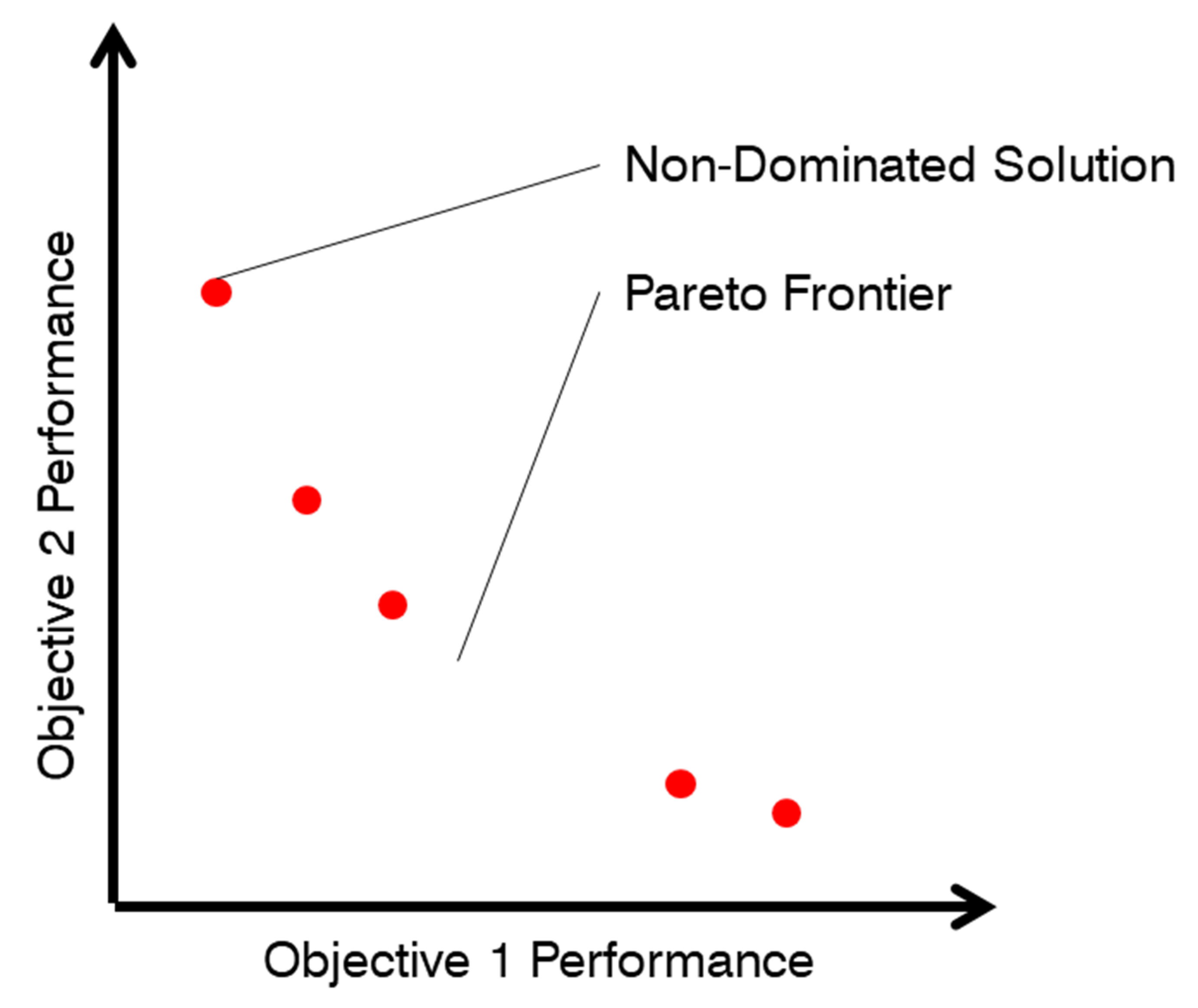
The simplest way in which to conduct multi-variate genetic optimization (i.e., with multiple cost functions) is simply to weight each function according to its importance. Problems often arise, however, when comparison occurs across multiple objectives that cannot be simply weighted. Kramer [10] describes a more nuanced method for finding a “non-dominated” or “Pareto-optimal” set of solutions. Solutions that can be improved upon in performance on at least one objective without harming the performance of another objective are said to be “dominated” or sub-optimal. Thus, the set of optimal solutions consists of all those solutions for which improvement of one cost function would result in worse performance on another cost function.

Solutions in which one objective can be improved without decreasing the performance of another objective are said to be “dominated” [10]. For problems with continuous variables and multiple objective criteria, there are infinite possible solutions, for which it is impossible to improve the performance of any one objective without harming the performance of another. This infinite set forms a “Pareto Front” [9]. Generally, using the sum of the weighted cost functions in multi-objective problems is impractical, as it necessitates running a large set of potential weights and is often computationally infeasible [9].

Fortunately, there are methods for handling a Pareto Front. These include (i) Schaffer’s vector evaluated GA, devised in 1984; (ii) Fronesca and Flemming’s multi-objective GA, devised in 1993; and (iii) non-dominated sorting GAs of the first and second type [9]. Figure 1 shows an illustration of a Pareto Frontier in a theoretical multi-objective problem.

For our multi-objective analysis described below, a non-dominated sorting genetic algorithm of the second type (NGSA II) is utilized. The intricacies of the NGSA II are explained in greater detail by Deb et al. [27].

For the purpose of this investigation, a random solution space is populated with 500 “solutions” or combinations of genetic variables (in this case, number of buildings and height, as explained below). Each of the 500 solutions is then evaluated based on either a single cost function (for single-objective optimization) or all three cost functions (for multi-objective optimization). The “fittest” solutions (i.e., those which have the best value in the cost function) advance to the next “generation”. Those solutions that perform poorly are culled. To populate the second generation, the best performing solutions from the first generation (above some threshold), undergo “crossover” and “mutation”. Crossover is the process by which the variable values for two separate solutions are combined. Mutation is the process by which one variable value is changed at random to produce a slightly modified solution, a process intended to avoid becoming “trapped” in local minima. Once again, each of the solutions of the second generation is evaluated using the cost function(s). The process then repeats until a certain condition is met. In this case, for a single objective, the algorithm terminates once 50,000 functions have been evaluated. For the more complex multi-objective algorithm, 1,000,000 function evaluations are performed.

While this process may adequately explain the single-objective algorithm, adding multiple variables adds an additional layer of complexity. In order to consider all three objectives simultaneously, each solution produced must be compared to all other solutions to find which solutions are “non-dominated”. Non-dominated solutions are those for which performance in one variable cannot be improved without performance in another variable suffering. Once the first front of non-dominated solutions is found, these solutions are temporarily discounted and the process is repeated (see [27]).

It is perhaps worth noting that while the genetic algorithm is widely used, it represents a heuristic and not an exhaustive search of the solution space. It is entirely possible that even a well-calibrated algorithm may not produce precisely optimal solutions.

2.1. Problem Definition

The site for our multi-objective analysis test case is on the near southwest side of the Chicago central business district (the loop). The 62-acre site is commonly referred to as “The 78”. An aerial photo of the site with its approximate dimensions is shown in Figure 2 below.

It represents a novel neighborhood scale problem in the growing area of “mega developments”. The site is bounded by Roosevelt Road to the North, Clark Street to the East, the South Branch of the Chicago River to the West, and Ping Tom Memorial Park to the south. It has been approved for the development of 13 million square feet of total gross floor area. According to the developer, the project this is a planned mixed-use community of “…new homes, commercial enterprises, cultural events, academia and outdoor recreational space…”.

The proposed algorithm will attempt to find an optimal combination of building quantities and heights for five building types in the neighborhood: for-sale residential, market-rate residential rental, affordable residential rental, office, and hotel. These five typologies are chosen as they account for the vast majority of tall building square footage in Chicago, with other uses (such as retail, education, place of worship) generally present in much smaller amounts in this type of building [28].

The number of buildings was limited to ten of each type, making a possible total number of buildings ranging from one to fifty. An ability to construct greater than fifty buildings would likely crowd the site to an unacceptable degree, given that it is only 62 acres. Floor ranges were limited between ten and one hundred. Ten was chosen as a lower bound as buildings of lesser proportion would be unsuitable for the urban nature of the site, which demands a certain level of density. One hundred floors were chosen as the upper bound, as exceeding this level is atypical, with only two completed or under-construction buildings in Chicago having greater than one hundred floors (Willis Tower at 108 and Vista Tower at 102) (Ibid.).

While a single building (let alone a collection of buildings) is potentially composed of an infinite number of design variables, some editing of the variables was required to draw meaningful conclusions from the results of the investigation. Use designation and height were chosen as these variables were believed to have a direct impact on the social, environmental, and economic cost functions prescribed. Other “high-level” variables, such as building shape and arrangement, may have had design impacts that were more difficult to evaluate with the proposed cost functions. A summary of the variables’ limits is provided in

Table 1. Summary of variables, upper bounds, and lower bounds.

Variable	Lower Bound	Upper Bound
Number of Market-Rate Apartment Buildings	0 Buildings	10 Buildings
Number of Condominium Buildings	0 Buildings	10 Buildings
Number of Affordable Housing Buildings	0 Buildings	10 Buildings
Number of Offices	0 Buildings	10 Buildings
Number of Hotels	0 Buildings	10 Buildings
Height of Market-Rate Apartment Buildings	10 Floors	100 Floors
Height of Condominium Buildings	10 Floors	100 Floors
Height of Affordable Housing Buildings	10 Floors	100 Floors
Height of Offices	10 Floors	100 Floors
Height of Hotels	10 Floors	100 Floors

.

Gross floor areas for buildings of each height were calculated using multiples of industry-standard leasable spans; residential and hotel floors were set at approximately 12,000 square feet, while office floors were set at approximately 36,000 square feet [29]. For simplicity, building shape was assumed to be a rectangular extrusion and the floor plates do not grow larger or smaller on a per floor basis regardless of the height of the proposed building.

The model accounts for the loss of floor plate efficiency (i.e., net floor area divided by gross floor area) implicit in taller structures. Based on the data from the literature, a linear regression model is used to determine floor area efficiency per floor height. Barton and Watts [30] provide efficiency values for buildings ranging from 0–50 stories and efficiencies ranging from 81–84% for “short” buildings to 75–79% for taller buildings. Sev and Ozgen [31] measured the floor plate efficiencies of ten tall buildings around the world with floor counts varying from 69–110 and efficiencies ranging from 60% to 77%.

Three cost functions were designed to evaluate the performance of each successive generation of the solution in terms of economic, environmental, and social sustainability variables. The economic cost function is generally based on rate of return as well as environmental on carbon impact, and social is determined by a social sustainability score. A penalty cost function is employed to ensure the suitable size requirements are met.

2.2. Economic Cost Function

Economic performance is evaluated using a simplified, single-term pro-forma, which seeks to maximize simple return on investment. For a project of this scale, real estate developers prepare much more complicated and nuanced multi-period models. Indeed, if one were to consider the “lifecycle” of the buildings’ finance in the same way as one may consider the “lifecycle” of the buildings’ energy demand, one would have to account for initial outflows for construction, land, soft costs, and entitlements. These would then be weighed against operating income from operations of less costs of maintenance, taxes, and debt service. Finally, a dispositional value associated with recursion would be calculated in some future period [32].

However, given that the pro-forma for each building type would vary and that the possible in-flows and out-flows for a thirteen million gross square foot development would be extremely complicated, even for professional financial modelers, development of a simplified method was necessitated.

Building costs are estimated on a per unit floor area basis using values from Marshall Swift Cost Estimation Calculator Method [33]. These include design fees, material and labor costs, sales tax, interest on building funds during construction, normal site preparation, grading, excavation, utilities, and contractors’ overhead and profit. Land costs are assumed to be static and are not considered because a single developer is in control of all the available lots for development. This may have the effect of showing shorter buildings more favorably, as high land prices tend to make taller buildings more attractive.

Per unit floor area costs are escalated using a “premium for height” factor. Costs tend to rise as the building height rises due to the increase in structure necessary to ensure rigidity, the cost of vertical communications, the cost of fire systems, and the cost of plumbing and electrical systems [34]. Inversely, groundwork, foundations, and roofing costs tend to decease with height, as each assembly is being divided over a greater floor area (Ibid.). De Jong and van Oss [35] calculate the premium for each ten floors to be 8% on a unit floor area basis. While this study focused on Holland and not Chicago, the model offered is sufficiently simple for the calculation method selected; also, applying the 1.008 multiplier (an 8% premium divided by ten total floors), a cubic relationship is achieved, rather than the simple linear relationship recommended by Marshal and Swift.

To find suitable values for market-rate apartment revenue, a survey of advertised rates in three recently completed or under construction buildings in the vicinity of the study site was conducted. This helped determine a “base” rent per net square foot of $3.39. To account for rental premium collected at higher floors, a linear regression model was used to measure prices against floor levels. The model outcome suggests that for each additional floor in height, renters are willing to pay $0.0155 per square foot.

For-sale housing unit prices were determined using a similar methodology. A survey of advertised prices in one recently completed and two under-construction projects in the vicinity were used to determine the price per net square foot (nsf) floor area of $431.43/nsf. Premium for height was again measured, in this case suggesting that each successive floor added $11.11/nsf of additional value.

For office space, rental rates ranges were taken from a squarefoot.com assessment of the apartment rentals in the vicinity. This metric shows rental rates for Chicago Class-A Office space in the range of $50 per net square foot. A height premium is less clear, with Barton and Watts (2013) noting that, “There can be little doubt that a tall office building attracts a premium of some nature, but articulating what that is, and how it relates to particular levels, would seem to be less than straightforward”. Koster et al. [36] found in Brussels, Amsterdam, and Utrect that “firms are willing to pay about 4% for a 10% increase in building height”. Further, they find that a “landmark effect” for buildings at least six times the average height is “about 17.5%”. Due to the lack of clear relationship and/or publicly available asking prices, a premium of 0.725% per floor is assumed. This value accounts for some modest rent premium while conceding the value is likely far less than that observed in residential spaces.

For hotel rooms, rental rates were taken from Chicago’s Average Daily Rate and Occupancy [37]. Each hotel room is estimated to be approximately 330 square feet [38]. To account for ancillary spaces for amenities, services, and circulation, a value of 450 square feet per room is utilized. No credible information on the premium for height can be found for hotels. Therefore, rooms on upper and lower floors are assumed to be equally desirable.

Affordable housing rents were also considered in our analysis. The City of Chicago’s Affordable Housing Ordinance [39] defines affordable rent as 30% of a net household income, which is 60% of the area median income, suggesting a total rent of $1026.05 per month. Divided by the average size of the observed units (972 square feet), this suggests a price of $1.05 per square foot. This value is not escalated based on height.

Office and residential properties must also account for vacancy. Office occupancy is estimated at 87% based on the Class-A occupancy rate for Chicago’s Downtown Market [40]. Apartment vacancies were provided by the Census’ American Community Survey, which suggests an occupancy of 94% for apartment units (a figure used for both market rate and affordable units).

Operating expenses were calculated as follows. For hotels, the per-key value for U.S. Limited Service Hotels was used ($21,390) [41]. For Apartments, the National Apartment Association Survey data is (excluding capital expenditures) was used ($9.12/square foot) [42]. For Office Buildings, the Building Owners and Managers Association per-square-foot operating expense were used ($12.47/square foot) [43].

Net operating income (i.e., income less expenses) was divided by the capitalization rate to find the net present value. Capitalization rates were taken from the Cushman and Wakefield Capitalization rate survey for Multifamily and Office Buildings for 2017. For hotels, the CBRE North American Capitalization rate survey was used. From the net present value, the initial cost can be subtracted to find the “profit”. This amount was then divided by the initial cost to find the rate of return. Rate of return was set to be maximized.

The economic cost function, then, seeks to maximize rate of return. Rate of return is defined as the net operating income divided by the capitalization rate less the initial cost of the solution. This number is then divided by the initial cost of the solution to provide a rate of return. Solutions with higher rates of return are considered “more optimal”.

2.3. Environmental Cost Function

The environmental cost function seeks to minimize greenhouse gas emissions over the course of the building’s life in the three enumerated categories. For the purpose of this investigation, such emissions are defined as the sum of the operational emissions, embodied emissions (at construction), and the transportation emissions of occupants. Other smaller environmental measures, such as air quality and water consumption, are not considered for the sake of simplicity. For simplicity, total greenhouse gas emissions of a given solution are the simple sum of fifty years of operational energy emissions, embodied energy of construction materials, and transportation energy used by occupants. A fifty-year building lifecycle is assumed for this calculation.

The energy assessment is not intended to be an exhaustive measure of all energy associated with the project. While operational energy and the embodied energy of materials can be somewhat accurately estimated using heuristics, other components of lifecycle energy use, including demolition, ongoing operations and maintenance, period capital expenditures, and recycling of building materials, are much more difficult to estimate accurately. As a matter of necessity, the system boundaries for this evaluation are based on operating energy, embodied energy of materials, and energy required to transport occupants.

This substantial simplification is necessitated by the level of design implicit to this investigation. It would be impossible to quantify, for example, the energy associated with steel erection without having a more completely designed building that is appropriate for this “high-level” exercise. A more robust lifecycle assessment (LCA), which would apply less restrictive system boundaries to a more completely designed set of buildings, would appear to represent a fertile area for further research.

Operational energy, or kilowatt hours of electricity, and therms of natural gas per square foot of floor area were calculated using the Department of Energy’s Energy Efficiency and Renewable Energy Office’s reference buildings for ASHRAE Climate Zone 5A. The “Midrise Apartment”, “Large Hotel”, and “Large Office” buildings were used for residential, hotel, and offices uses, respectively. Greenhouse gas emissions were calculated from energy quantities multiplied by site-to-source factors and input into the Environmental Protection Agency’s Greenhouse Gases Equivalency Calculator.

Embodied energy was limited to the embodied energy of buildings themselves and does not consider the embodied energy of infrastructure. Once again, a per-unit-floor area method is utilized. Theil et al. [44] evaluates embodied energy values for five existing tall buildings, with heights varying from three to 38 floors. Evaluation of these precedents suggests a “baseline” figure of 0.325 tons of CO2E per gross square foot. As noted with respect to efficiency, taller buildings require a greater amount of structural materials due to the increasing lateral loads. Foraboschi et al. [45] investigated the relationship between embodied energy and height for buildings between 20 and 70 floors. By conducting a linear regression on the buildings they survey, a premium for height can be conducted.

While this escalation would theoretically only hold true for structural materials, no suitable values are found in the literature for finish or envelope materials. As structure is believed to represent a “worst case scenario”, this escalation factor is applied to the total embodied energy cost. Embodied energy associated with ongoing capital expenditures are not well defined in the literature and are excluded.

To be clear, the embodied energy of construction materials was calculated by multiplying a per-square-foot embodied energy total for tall buildings by an escalation factor for height provided by the literature (as taller buildings require more materials per unit floor area to construct).

Transportation energy was based on the number and type of occupants. According to the US Department of Transportation (2019), per capita fuel consumption in Chicago, IL, measures 206 gallons of gasoline and 37 gallons of diesel fuel per person. For residential projects, the number of occupants was defined by dividing the net square footage of each building by the average unit sizes. This was then divided by the average United States household size of 2.6 occupants [46] to find an occupants per square foot factor. For offices, the Commercial Real Estate Development Association tracks the number of net rentable square foot per office employee [47]. The number of occupants can be found simply by dividing net floor area. For hotel rooms, 450 square feet per room was assumed, with 1.6 occupants per room. The latter number accounts for both direct occupants and staff, which are estimated at 0.5 to 1.0 persons per room [48].

Occupants are assigned an occupancy factor based on the amount of time they are expected to spend in the building. For example, a typical office worker is assigned a factor of 24%—40 h of office work per week out of 168 total hours. Similar calculations were done for hospitality and residential usage. The occupant number was multiplied by each occupancy factor for the total number of occupants.

The environmental cost function seeks to minimize the sum of the operational, embodied, and transportation greenhouse gas emissions. The cost function for environmental performance of each solution, then, was simply the sum of the following calculations:

○

Fifty years of greenhouse gas emissions associated with the generation of energy to serve operational needs of the building.

○

The greenhouse gas impact of the construction materials (embodied energy), calculated on a height-escalated per-unit-square-foot basis.

○

The greenhouse gas emissions associated with generation of energy to support vehicular transportation of occupants, as assigned above.

The environmental cost function seeks to minimize this sum number. Solutions that have less total greenhouse gas impact are considered more optimal than those with greater greenhouse gas emissions.

More robust tools for true lifecycle assessments exist. Monahan and Powell [49], for example, used a cradle-to-site approach to more accurately measure design alternatives regarding carbon impact from the extraction of raw materials through their processing and installation. Dodoo et al. [50] investigated the lifecycle carbon emissions associated with cross-laminated timber construction, finding that the “low-energy” method of construction reduces lifecycle greenhouse gas impacts by 9% (excluding operational electric and water heating energy). Sansom and Pope [51] focused more completely on the lifecycle embodied energy impacts of steel buildings, using the CLEAR model. While this model includes material manufacture, transport, construction waste, transport of waste from site, construction process energy, and end-of-life recovery, it does not include demolition/deconstruction energy or maintenance energy. In each of these cases, complete building designs or already constructed buildings are used to construct a more robust inventory of lifecycle carbon impacts. Unfortunately, the “early schematic design” nature of the problem investigated does not offer such complete information on buildings. This represents a potential weak point in our analysis.

At first look, it may seem as though such a function would prefer to build zero square feet, with each additional square foot having a penalty. This is addressed below in the discussion of penalty functions.

2.4. Social Cost Function

Of the three objectives considered, the social objective is by far the most difficult to quantify. A survey of the literature finds common markers of social sustainability, often referred to as Social Sustainability Performance Indicators [52]. The indicators that occurred most frequently in the literature were then matched up against the variables considered to see if they would have any impact. For example, while democratic social governance may be critical to social sustainability, it is not clear that it is affected by building uses or heights. Therefore, only suitable indicators that could be quantitatively impacted by the chosen variables were considered. In all, three markers met this set of criteria, namely, housing affordability, employment opportunity, and tax base.

Of the social criteria considered, perhaps the most directly supported in the literature is the call for some component of affordable housing. Kamali and Hewage [52] cite affordability among their Social Sustainability Performance Indicators (although not explicitly “affordable housing”). Stender and Walter [53] explicitly include affordable housing in the accessibility portion of their Social Sustainability Framework. The provision of shelter is cataloged among signs of the development of equity in Murphy’s [54] analysis, which also notes that housing provision is among the social “themes” of the United Nations Commission for Sustainable Development. Eizenbern and Jabareen [55] suggest inclusion of a greater diversity of housing types and incomes promotes social sustainability. Al-Kodmany [56] cautions against the creation of tall buildings solely as “mansions in the sky”, which are said to “reinforce social and racial segregations”.

More abstract than the direct provision of affordable housing is the notion that socially sustainable development should offer prospects for employment, thus contributing directly to the economic well-being of the host city. Kamali and Hewage [52] suggest that contribution to the local economy is a key Social Sustainability Performance Indicator. Broman and Robert [57] indicate that social sustainability requires that people “are not subject to structural obstacles to competence”. Others are more direct in connecting employment to social sustainability. Murphy’s [54] literature review of the “Pillar of Social Sustainability” finds numerous suggestions of the importance of employment opportunities. Stender and Walter [53] include employment along with education amongst their “Accessibility” categories in their social sustainability framework. Eizenbern and Jabareen [55] identify a connection to employment, although they see it as a “non-physical” component.

While the benefits of jobs and affordable homes can be easily seen as social goods, the idea of developing more value for taxation is more abstract. The immediate consequence of taxation is not particularly beneficial, but the schools, transportation network, and redistributive policies that taxes pay for can be of immense social benefit.

Of the Social Sustainability Performance Indicators identified by Kamali and Hewage [52], many appear immediately connected to benefits typically funded through taxation. Specifically, the health of occupants, influence on location social development, cultural and heritage conservation, safety and security, and neighborhood accessibility and amenities are directly connected to taxes. Landmarks Ordinances, Police Patrols, Parks, and Public Transit access all are funded, to some degree, through local taxation. The security against crime, fire, and earthquakes, recommended by Maleki et al. [58], can be seen as analogues for well-funded police departments, fire departments, and code enforcement officials. Amenities, connection, and safety are keys to the “Social Cohesion” component of Stender and Walter’s [53] Social Sustainability Formwork. Once again, it seems a key provided of physical access, physical safety, and neighborhood-scale amenities is the local government. The Framework for Strategic Sustainable Development [57] promotes removal of obstacles to free speech, education, and partial treatment. Such justice and education outcomes are inexorably tied to locally funded government. The participation and social cohesion axes identified by Murphy [54] and the safety and equity axes identified by Eizenbern and Jabareen (2016) appear similarly connected to the public sector.

In each case, a factor can be calculated comparing the amount of social good provided by a given solution relative to the maximum possible social good. For example, the affordability factor asks what percentage of affordable housing is provided relative to the total development. In this case, the maximum possible is 100% of the development is built with affordable housing units. For employment opportunities, what amount of employment is generated compared to a development which is entirely comprised of offices (the most employment intensive use). Finally, tax base seeks to find what percentage of net present value (the basis for property taxes) is provided vs. the system with the greatest net present value. The total Social Sustainability Factor is a simple weighted average of these three metrics (affordability is assigned the highest weight due to its prominence in the literature).

The Social Cost Function by which each prospective solution is evaluated, then, consists of the sum of fraction of all possible employment provided by the solution, the fraction of all possible tax revenue provided by the solution, and two times the fraction of all possible affordable housing provided by the solution, divided by four. As the amount of affordable housing, tax base, and employment opportunities increases within a solution, the value of this Cost Function will go up. Thus, solutions that have greater opportunities for affordable housing, employment, and tax base will be considered more optimal than those with less such opportunities.

2.5. Penalty Functions

It is possible for the solution set to produce a wide range of potential square footages. Local ordinances, however, allow a limit of approximately 13,000,000 gross square feet in total for all uses. Therefore, in order to ensure solutions that will build near this square footage are prioritized, penalty functions are introduced to each objective cost function. A penalty function was chosen over a simple constraint because a penalty function can “nudge” solutions towards the desired gross floor area, thereby making a potentially good solution more fit over the generations, rather than simply discarding it.

For example, the environmental cost function, for each square foot greater than 13,500,000 square feet or less than 12,500,000 square feet, a penalty is imposed. This is intended to “direct” the evolving scenarios towards the appropriate square footage. A similar principle is used for the Sustainability Score cost function, albeit of a much lower magnitude. In these cases, each square foot subtracts a penalty from the cost function outcome. The same value is applied to the return on investment cost function in the economic model.

These values are calibrated toward solutions of the desired square foot total. Using penalty functions that are too large causes the model to converge on solutions with the correct floor area without sufficient regard of their performance in the objective cost function categories. Using penalty functions too small does not penalize solutions enough, allowing them to exceed square foot limitations.

2.6. Model Scenarios

In this study, data are provided for four scenarios: (A) Economic Optimum; (B) Environmental Optimum; (C) Social Optimum; and (D) Combined Optimum. These scenarios offer a mix of single-objective optimization for a single cost function, and a multi-objective optimization combining all three cost functions to define the Pareto Set. The single-objective scenarios are designed to converge at a singular solution, while the multi-objective scenario will provide a set of non-dominated solutions.

Three single-objective scenarios will evaluate a breadth of solutions based on each of the cost functions enumerated above (one each for social, environmental, and economic sustainability). Settings for the single-objective runs are shown in

Table 2. Single-objective genetic algorithm input settings.

Setting	Value
Algorithm	Standard Genetic Algorithm
Seeds and Repetition	Random Seed (Mersenne Twister)
Termination Criteria	Perform 50,000 Function Evaluations
Initial Population	500
Selection Method	Tournament Selection with Tournament Size Ten
Crossover Method	Double Crossover with a Probability of 0.7
Mutation Method	Jump (Probability 0.1) and Creep (Probability 0.75) with Elitism of 1

below. The table defines the input values that were used to construct the genetic algorithm, such as the probability that a given solution is changed (“mutated”). A single multi-objective run simultaneously considering all cost functions was also performed. The settings for the multi-objective algorithm are given in

Table 3. Multi-objective genetic algorithm input settings.

Setting	Value
Algorithm	Non-Dominated Sort Genetic Algorithm II
Seeds and Repetition	Random Seed (Mersenne Twister)
Termination Criteria	Perform 1,000,000 Function Evaluations
Initial Population	500
Crossover Probability	0.5
Mutation Probability	0.5
Mutation Rate	0.02
Mutation Sigma	0.1

.

An understanding of the general operation of the model and the underlying cost functions will help to contextualize the results.

3. Results

Following are the results of our four scenario optimization analyses.

3.1. Scenario A: Economic Optimum

The average of the cost function values (simple rate of returns) for the initial population was between 0.250 and 0.275. The best solution found was found in Generation 107. This solution (Figure 3) had the improved value of 0.503 (or 50.3% return).

Unsurprisingly, the optimum economic solution contains no affordable housing, as the rent for such housing is considerably lower. The inclusion of hotel and office buildings of lesser height in the solution is also unsurprising, given that lower heights are where returns are maximized for these typologies. Apartment buildings are taller due to the rent premiums commanded for taller units. A single condominium building helps the solution reach 13,000,000 square feet. Its inclusion is likely due the limitation put on building type (a maximum 10) and adding height to these buildings would harm their economic prospects due to increasing the costs and lowering efficiencies.

3.2. Scenario B: Environmental Optimum

The environmental optimum improved on green-house gas emissions, using 13,394,795 MT CO2E (lifecycle) emissions; this is one tenth of the average baseline values. While the economic model took 107 generations to find its optimum, the environmental model was not able to improve upon the environmental solution found in the 17th generation (Figure 4).

In this solution, residential uses dominate. This is because they have the lowest per unit floor area lifecycle energy consumption compared to other uses. The preference for condominiums over apartments and affordable residences is also explained by a smaller footprint of the building type. Condominiums offer a mix of low operational energy and fewer occupants; with fewer persons per square foot, transportation emissions are reduced. Taller buildings are also selected as part of this optimum. The embodied energy inherent in taller buildings appears to be overwhelmed by their other “energy-saving” characteristics.

Market-rate apartments and affordable housing are basically interchangeable in terms of energy use, so a preference for one or the other is a matter of chance. The inclusion of a single, minimum height office building is unexpected, given the energy-use intensity of these buildings.

3.3. Scenario C: Social Optimum

The initial population’s average values for the combined Social Sustainability Factor were actually negative, measuring between −0.45 and −0.50. The length of the simulation required to produce the optimum was 34 generations. The best solution (Figure 5) had a social sustainability score of 0.354.

Given the focus of the social score on providing affordable housing, it is unsurprising that most buildings in this configuration are affordable apartments. The inclusion of offices, which are the most job-intensive of the modalities considered, is also reasonable. The provision of a single, very tall apartment tower is a bit more difficult to justify, although apartment buildings typically have high net present values, generating high tax revenues. This and a declining efficiency in taller buildings makes market-rate units less attractive. Since the model considers the percentage of total housing units that are affordable rather than the absolute number of units, an aversion to construction of market-rate units is expected. The inefficiency of taller building floor plates may be the only factor limiting the model from selecting even fewer taller buildings.

3.4. Scenario D: Multi-Objective Optimum

From the population of 500 individuals, a model combining all 3 objective cost functions produces a set of 161 non-dominated solutions. This means there are 161 solutions discovered for which it is impossible to improve the performance of any one objective without harming the performance on another objective. Figure 6 shows the Pareto surface in a three-dimensional form, with performance on each axis normalized.

Normalization was accomplished by eliminating all duplicate solutions. To allow for a more direct comparison of each objective function, the non-dominated solutions’ cost function values were arranged linearly on a scale from zero to one, with zero representing the least desirable score, and one representing the most desirable score.

The 161 novel solutions provide a fairly wide variety of answers to the question of which combination of buildings and heights is optimal.

Table 4. Population information for the first-rank solutions.

	Apart. Number	Condo Number	Afford. Number	Office Number	Hotel Number	Apart. Height	Condo Height	Afford. Height	Office Height	Hotel Height
Min	1	1	0	0	0	46	35	28	20	19
Max	9	8	8	5	3	97	72	53	59	42
Avg	7.78	4.23	2.76	2.04	0.04	80.94	45.65	38.61	25.39	36.23
Med	8	4	2	2	0	85	45	39	24	36
Std Dev	1.15	1.83	1.99	1.36	0.33	13.22	6.43	5.67	5.00	3.52

summarizes the characteristics of the solution set.

The non-dominated solutions appear to have selected from a wide range of possible building number combinations, especially for residential projects, which show the greatest degree of variation between total building counts. For offices and hotels, the variation is less, with no solution opting for more than five offices or three hotels. The average number of hotels is also noteworthy. While the range of outcomes was between zero and three, the average of only 0.04 suggests that most solutions had no hotel use at all. Hotels may be hampered by providing relatively poor environmental performance and relatively few jobs. Offices have stronger employment numbers, but their weak environmental and economic performance likely contributed to their exclusion as a major part of many solutions.

By number, the highest average and median belong to apartments, then condominiums, and finally affordable housing. Apartments offer strong economic performance and ecological performance that is better than offices or hotels. Condominiums are a slightly weaker economic prospect but have superior environmental performance due to their lower number of occupants. Affordable housing was likely selected due solely to its impact on social variables.

In terms of building height, the tallest building of any solution was a 97-story apartment building. Generally, apartments had the highest average and median heights, possibly because of rent premium paid for heights in residential projects. It is also worth noting that market-rate residential had the highest standard deviation, suggesting a wide spread between the tallness of these buildings between the non-dominated solutions. Affordable housing tended to have lesser height, likely because rents are not responsive to height. Hotels and offices were built only in the most economic (i.e., least expensive) cost ranges.

3.5. Results Evalation

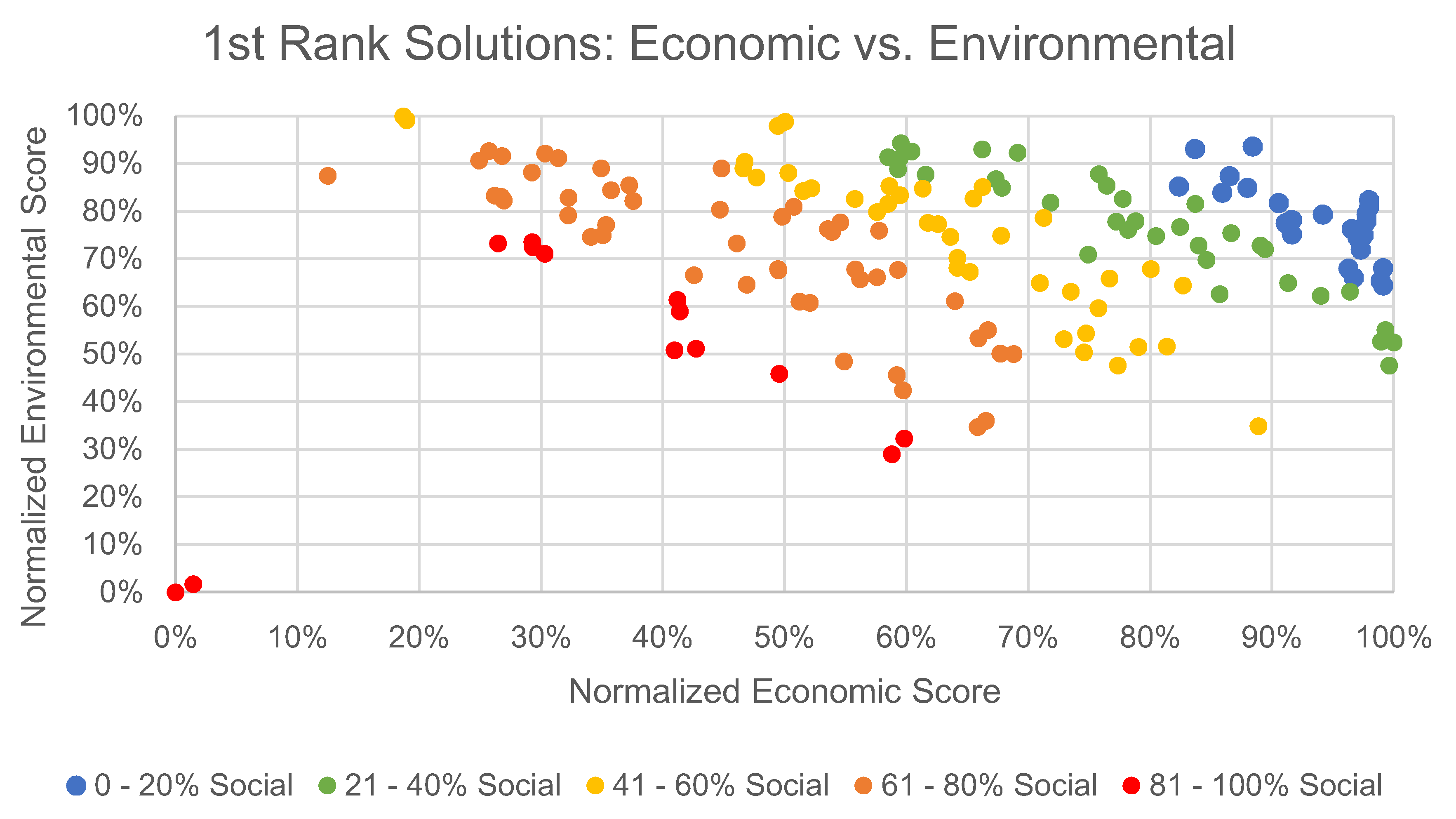
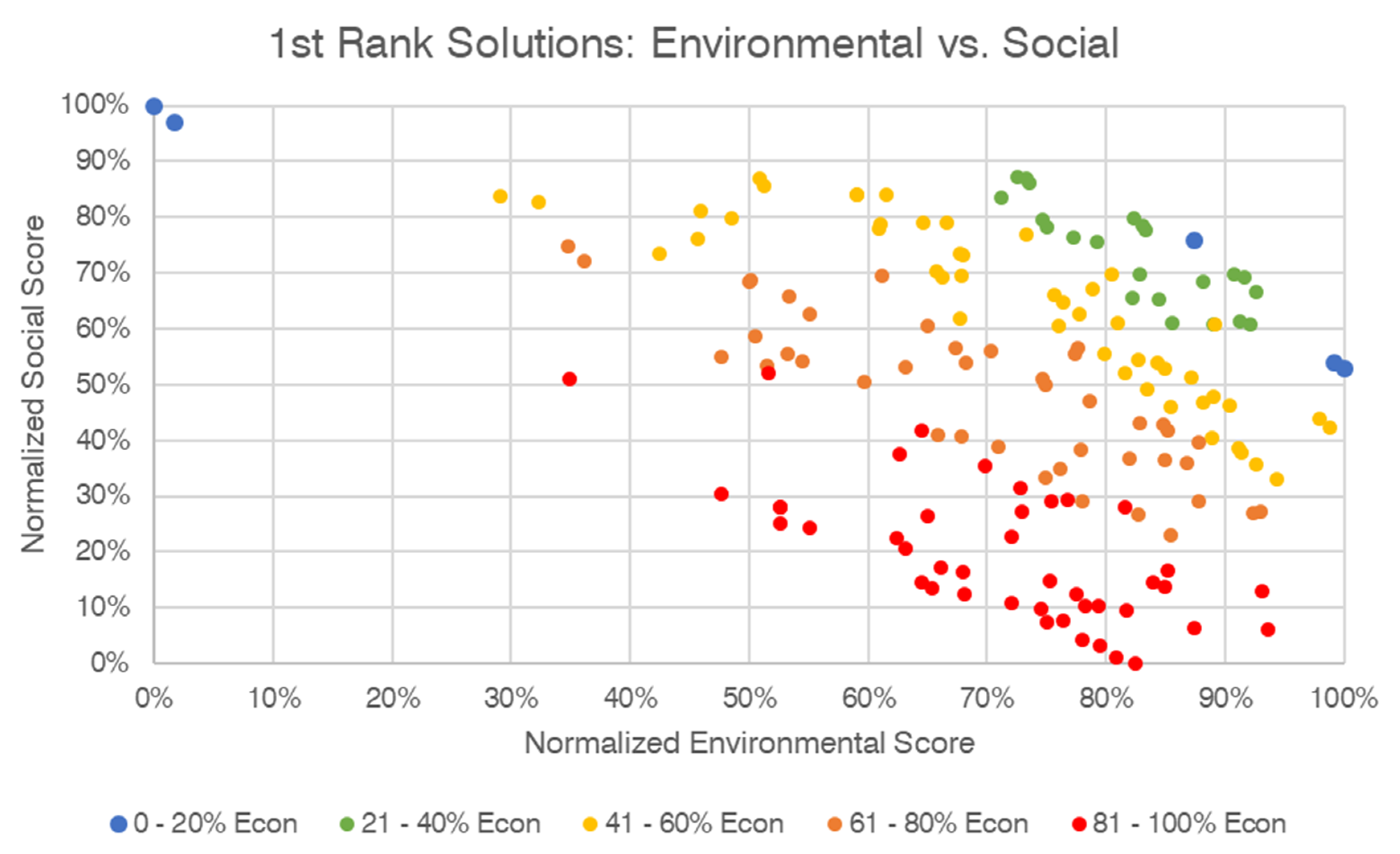
It is fairly difficult to draw any inferences about the solution set from the three-dimensional figures alone. A two-axis point cloud in which the “third dimension” is provided by color may be more telling. Figure 7, Figure 8 and Figure 9 provide such an analysis. Figure 7 compares economic to environmental performance. Figure 8 compares economic and social performance. Figure 9 compares environmental and social performance.

Evaluation of the solution set on only economic and environmental variables shows that the variables may be correlated, but weakly. While few solutions have poor scores in both economic and environmental performance, solutions with strong performance in one category may have only moderate performance or even weak performance in another. Given the right-weighted distributions seen in the histograms above, the trade-off between environmental and economic performance does not appear as straightforward as the other comparisons below. Some solutions were able to perform well in both economic and environmental score.

A much stronger correlation is shown between the economic and social scores. Solutions with strong economic performance tend to have poor social performance. Likewise, solutions with strong social performance tend to have poor economic performance. The absence of any data points in the upper right of the graph suggests that no solution was able to harmonize economic and social performance. This suggests that the trade-offs between economic and social performance are more direct and primary, and that the trade-offs between economic and environmental performance are more secondary in nature.

The relationship between social and environmental performance appears to be neither as strongly correlated as that between economic and social performance nor as loosely correlated as that between economic and environmental performance. While the bareness of the lower left quadrant in the graph does suggest that few solutions had poor performance in both categories, some solutions appear to have performed fairly well in both. This would suggest that environmental and social performance are not mutually exclusive, although some trade-off between environmental and social performance is observed.

Returning to the Planners’ Triangle, our analysis for this problem supports the notion that economic and social objectives (the “Property Conflict” in Campbell’s parlance) involve substantial trade-offs and that strong performance on one of these objectives tends to limit performance on the other. The conflicting goals of environmental and social objectives (the “Development Conflict”) are not as strong in the model. Finally, economic and environmental objectives (the “Resource Conflict”) do not appear to be at odds, with environmentally performative solutions running the gamut between poor and strong economic performance. This suggests that, of Campbell’s conflicts, the Property Conflict is the most pronounced and the Resource Conflict is the least pronounced for the problem explored.

The method utilized shows promise for understanding the trade-offs between each of the three nodes of sustainability and suggest that quantitative investigations of these trade-offs is possible. To the extent that design problems can be broken into variables and their performance evaluated with cost functions, it seems likely that optimization would offer a strong method of evaluating potential solutions.

4. Discussion

The proposed method demonstrates promise in helping designers to balance the competing objectives of social, environmental, and economic performance. As performance across these variables becomes more critical to design, tools capable of creating and measuring such a balance become important.

Considered cumulatively, the Planner’s Triangle provides a useful formwork for optimization across three sustainability-oriented objectives. However, the method described here need not be limited by this scaffolding. Trade-offs between safety, economy, sustainability, and other metrics of performance could be designed for different problems.

Consideration of the neighborhood scale is also important, given the proliferation of the “mega project” as an architectural typology. In reality, multiple “nested” optimization methods may be required for architectural design, with a high-order optimization method such as that proposed herein offering only a first step to smaller scale optimization in programming, massing, and detailing.

On the whole, the model provides a useful framework for understanding the trade-offs that are implicit in architectural design at the neighborhood scale, particularly as it relates to the competing objectives within the notion of “sustainability”. It also raises questions about the use of traditional, eminence-based design methods in architecture. Finally, it suggests a method by which architects and designers may add quantifiable rigor to their design process.

The results may be unique to the design problem, but the method can be useful to designers seeking to make informed, quantitatively valid decisions during the early phases of project programming and development. The range of acceptable solutions can provide constraints useful to the design process, helping in narrow the field of the designer’s choices from an infinite solution space to a smaller set of possibilities.

Drawbacks and Limitations

Expanding this method to a more diverse set of problems, rather than the single problem explored in this paper, is an important area for future research. While the findings of this paper suggest that the tool explored is useful to designers, it is not difficult to imagine problems that would be more difficult to distill into variables and cost functions. Given the complex nature of design problems, more complex and sophisticated models with a greater number of variables and more elaborate cost evaluations may be required to understand problems in more granular detail.

The method is also reliant on the quality of the evaluations performed. More research is needed to ensure that the cost functions have strong external validity, especially in the case of the social sustainability score, which represents something of a bespoke solution. Modifying the cost functions, even subtly, can have a high degree of impact on the non-dominated solutions discovered.

While single-objective cases intuitively seek to select a single solution, multi-objective models can, by definition, only provide a set of non-dominated solutions. As architects and designers are typically permitted to build only one solution, a method would need to be devised to pick between the non-dominated solutions proposed. This suggests that such an optimization model would have to be part of a larger, integrated design process and may be incapable of arriving at any sole “optimal” condition without the continued input of designers.

Opportunities for improvement exist, both within the framework proposed here and as an expansion of the framework to other problems. More research is needed on the idea of premium for height, which has only been explored in certain contexts and situations. A more complete understanding of how height changes performance across all three objectives considered herein would add validity to the model. The social and economic sustainability of buildings of variable height appears to be an area particularly bereft of empirical research. More research is also required in understanding the longitudinal variables implicit to urban problems. The model, as shown above, assumes all buildings are built and sold instantly. In reality, the completion of an urban project of this scale may take a generation, with parameters for “success” changing along the way. Similarly, the time necessary to design, construct, and stabilize solutions requires a more nuanced treatment.

Social sustainability indicators are also not quantitatively understood as they apply to buildings and collections of buildings. While the literature suggests social sustainability indicators are robust, a concerted effort to create some externally valid and reliable measure of social sustainability for use within and between projects would appear to be a fruitful area for future research. In order to have wide applicability to architects, more research is necessary to attempt to quantify how such multi-variate optimization performs at smaller (e.g., single building or detail) and larger (e.g., cities and regions) scales.