Article

Traffic State Estimation and Classification on Citywide Scale Using Speed Transition Matrices

Faculty of Transport and Traffic Sciences, University of Zagreb, HR-10000 Zagreb, Croatia
*
Author to whom correspondence should be addressed.
Sustainability 2020, 12(18), 7278; https://doi.org/10.3390/su12187278
Submission received: 29 July 2020 / Revised: 28 August 2020 / Accepted: 1 September 2020 / Published: 4 September 2020

Abstract

:
The rising need for mobility, especially in large urban centers, consequently results in congestion, which leads to increased travel times and pollution. Advanced traffic management systems are being developed to take the advantage of increased mobility positive effects and minimize the negative ones. The first step dealing with congestion in urban areas is the detection of congested areas and the estimation of the congestion level. This paper presents a a method for a traffic state estimation on a citywide scale using the novel traffic data representation, named Speed Transition Matrix (STM). The proposed method uses traffic data to extract the STMs and to estimate the traffic state based on the Center Of Mass (COM) computation for every STM. The COM-based approach enables the simplification of the clustering process and provides increased interpretability of the resulting clusters. Using the proposed method, traffic data is analyzed, and the traffic state is estimated for the most relevant road segments in the City of Zagreb, which is the capital and the largest city in Croatia. The traffic state classification results are validated using the cross-validation method and the domain knowledge data with the resulting accuracy of 97% and 91%, respectively. The results indicate the possible application of the proposed method for the traffic state estimation on macro- and micro-locations in the city area. In the end, the application of STMs for traffic state estimation, traffic management, and anomaly detection is discussed.

1. Introduction

Demographic, economic, and technological changes and developments are enablers that support the increase in the human need for mobility, especially in large urban centers. The increase in the need for mobility leads to advanced solutions in the traffic management domain and requires the implementation of Intelligent Transport Systems (ITS) solutions and applications [1]. Aside from the positive effects, it also has negative effects, such as increased congestion or pollution in urban areas.
The sustainable transport development is often confronted by a traffic congestion. The European Commission reports that congestion that is caused by increased mobility accounts for 40% of all CO 2 emissions of road transport and up to 70% of other pollutants from transport, and the total cost of congestion in the EU is nearly 100 billion, which stands for 1% of the annual EU’s GDP [2]. Traffic congestion can be classified as recurrent, mostly due to a large number of commuters during peak hours, and non-recurrent caused by an unexpected event, such as traffic accidents, extensive weather conditions, or special events. The authors in [3] report that recurrent congestion traffic covers almost 85% of all congestion occurring on the urban road networks. On the other hand, different numbers are reported for the highway facilities [4], where the authors state that 50% of all traffic congestion is caused by non-recurring congestion and 40% is caused by recurring congestion. The crucial part of ITS supported systems for the decision-making processes are the detection and quantification of traffic state to initiate and implement improvement strategies. Moreover, traffic state estimation is a prerequisite to many other ITS applications, like travel time prediction [5], route computation [6], traffic flow prediction [7], etc.
This paper presents a method for the traffic state estimation on urban road segments that are based on the clustering of the Center Of Mass’ (COMs) of the speed data represented in the Speed Transition Matrices (STMs). The proposed methodology includes three main steps: (i) data preprocessing, (ii) STM computation based on the speed data, and (iii) clustering-based traffic state estimation process. The main part of the preprocessing step is data filtering based on the seasonality that results in summer months and weekend data being excluded from the real-life large Global Navigation Satellite System (GNSS) dataset. The STMs were computed based on the speed data, and they represented the speed probability distribution of vehicles traveling between two road segments (transition). Next, the agglomerative clustering approach is conducted in order to cluster the traffic data in form of the STMs. Clustering results in three classes of the traffic state. The results are validated using the cross-validation approach and the specific domain knowledge data, which were extracted from the Highway Capacity Manual (HCM). The validation resulted in the average accuracy of the classification for the cross-validation of 97%, and the domain knowledge data in 91%.
Contributions of this paper are as follows:
-
Novel traffic data representation is proposed in form of the STM which application is shown for the traffic state estimation, routing applications, and anomaly detection.
-
The methodology for the traffic state estimation on a city-wide scale is proposed based on the STMs and computed COMs.
-
The proposed methodology is applied and validated on the real dataset for the City of Zagreb, Croatia.
The rest of the paper is organized as follows. In Section 2 literature review is presented on recent developments related to GNSS data representation, data modeling techniques, and traffic state estimation approaches. Section 3 presents the methodology that was used to estimate the traffic state using the STMs and computed COMs with clustering, and validation methods. Section 4 describes the used real-life GNSS dataset and the results of traffic state estimation, clustering, and validation. In Section 5, the discussion is given regarding the presented method for the traffic state estimation. The advantages and disadvantages of using the proposed methods are given, and the possible application of the STMs for other traffic-related problems are presented. Section 6 presents the conclusion and future work suggestions.

2. Literature Review

2.1. GNSS Data for Traffic Representation

The crucial part of the ITS are data-driven services [8,9], which are supported by the advancements in technologies that enabled the lower cost of data collection systems. There are roughly two groups of data collection systems: (i) dedicated infrastructures which mostly consists of point detectors such as loop detectors, radar or lidar counters, and traffic cameras, and (ii) Floating Car Data (FCD) with devices mounted inside vehicle or carried by the driver, like GNSS devices or cellular data. The FCD from GNSS devices is often used to collect traffic data, because it provides a low cost, high accuracy, less delay, and wide coverage. One of the main FCD advantage is the ability of route construction and analysis.
The authors in [10] used GNSS data to conduct a field experiment in order to validate collected traffic data. The result suggests more reliability when using the GNSS data than loop detector data. In [11], the authors conducted an experiment with mobile phones onboard GNSS devices for traffic density and volume estimation. The results show that the proposed models successfully incorporate GNSS data to estimate the traffic parameters. In [12], the authors used GNSS probe data for the traffic state estimation based on the speed by incorporating the curve fitting method. In [13], the authors used streaming GNSS data to classify the travel modes based on the characteristic distribution of velocity and acceleration for different travel modes.
The GNSS datasets enable the use of the dynamic routing applications. Dynamic routing can be defined as a process of changing the original (pre-computed) route based on the current traffic state on the road traffic network [14]. The traffic network’s dynamic nature is manifested in both temporal and spatial changes that can be captured by GNSS data. The authors in [15,16] conclude that drivers with available real-time traffic information can significantly decrease travel time if compared to the drivers using offline navigation tools.
In this paper, FCD data that were based on the GNSS tracks were used. The data were preprocessed to compute the STMs that present the speed probability distributions when vehicles are moving between consecutive road traffic segments. Computed STMs were used to represent the traffic state on the observed road network segments. The STMs can be used in both offline and online route planning scenarios.

2.2. Data Modeling Techniques

When estimating traffic states from sparse GNSS datasets, most of the authors use aggregation-based methods in order to determine the observed traffic parameter value. Traffic data, like speed, volume, or density, are mostly aggregated in profiles that represent the change of observed parameter over the defined time period, i.e one day. Data is usually aggregated in a narrow time interval (common values are 5-, 15-, 30-, 60-min.) as an average or median of all values recorded in the observed time interval. Because of the data aggregation, profiles could include large deviations in some time intervals that raises the question of the reliability of obtained results. One more challenge in data aggregation is related to the missing data, as it can extremely influence the average or median values.
Vector representation of traffic data in the form of a time series is one of the most common data modeling techniques [17]. The change of traffic parameter under observation with dimensions 1 × n is examined through a daily profile in defined n time intervals. The shortcomings of such approaches are reflected in the inability to represent spatial components of the observed parameter. In contrast, some authors, [18,19], used matrix models in order to represent the traffic data. Matrix models can model more complex data, with the ability to represent more dimensional data. Then, both spatial and temporal information can be analyzed simultaneously. In most cases [18], matrix dimensions are represented with m × n where m represents the number of spatial segmentations (often road segment) and n number of time intervals. This kind of modeling can be used to extract spatial and temporal dependencies between the observed traffic parameters. For example, in the case of the commonly used data representation form of Origin-Destination (OD) matrices, one more dimension must be added in order to analyze the temporal component. OD matrices represent the number of vehicles traveling between defined points in the traffic network. While the provided information is useful for mobility pattern research, the patterns could indicate false information due to the predefined delivery routes if the data consist of delivery vehicles.
The novel data representation in the form of STM is proposed in order to overcome the mentioned limitations regarding the sparse GNSS data analysis. STM does not suffer from aggregation or missing data limitations, as data are not aggregated in such a way, and all of the recorded speed data are shown in one matrix. The origin and destination vehicle movement are limited to consecutive links, enabling the usage of delivery vehicles in the traffic analysis process.

2.3. Traffic State Estimation Approaches

Many traffic state estimation approaches are developed to overcome the challenge of quantifying the congestion on the road networks [20]. Measures are related to the available traffic parameters, such as speed, travel time, congestion indices, delay, volume, and level of service. In this paper, the speed is chosen as a traffic parameter for traffic state estimation. The authors in [21] report that speed is a good measure for traffic state estimation, because the congestion is a function of speed reduction, which is related to increase in time travel, vehicle operating cost, fuel consumption, and emissions. When using the GNSS data, the speed is relatively easy to compute and does not require complex processing if compared to extracting the traffic volume from the same dataset [22].
One of the main research goals with a topic that is related to traffic state estimation is to discern different states and provide a certain threshold for the classification of the traffic states. The well-known traffic study [23] presents the three-phase traffic theory. It includes classification to three states, namely “wide moving jam”, “synchronized”, and “free flow”. The additional research was presented in [24], where the authors presented a method for tracking synchronized flows and propagating moving jams. The authors in [25] classified the congestion based on the traffic images that represent speed on the observed road segment, resulting in five classes, namely “isolated”, “low frequency”, “high frequency”, “homogeneous”, and “mixed”. In [26], the authors used a clustering technique to estimate the traffic state based on the trajectory data. The authors in [27] used artificial neural networks and decision tree algorithm to classify road traffic congestion levels based on the extracted speed traffic patterns. The research resulted in three classes, namely “jam”, “heavy traffic”, and “light traffic”. In [28], the authors used neural network to classify traffic patterns with the aim of incident detection. The authors report three classes of traffic state described with speed, volume, and occupancy values. The authors in [29] estimate the congestion of the trajectory segments with three different intensities. Subsequently, congestion events are identified in the traffic network on each turning direction through multiple clustering approaches based on the speed, distance, and time of day. The authors in [30] aim to visualize the traffic conditions on the urban road network. Traffic conditions are classified based on the average speed and grouped into five different classes.
In this paper, three classes of traffic state were used, namely “Free flow”, “Stable flow”, and “Congestion”. This approach is used to characterize the congested traffic state and describe all of the states that can occur on the traffic network. The COM estimation process is used to simplify the clustering process of traffic data that are represented by STMs. The three dimensional STM representation is transformed into the two-dimensional representation using the x and y coordinates of COM. With this transformation, the classical distance metric, such as euclidean distance, is more interpretable than the classification of raw matrices, where distance is measured between every cell in two matrices. The proposed approach presents a simple but effective way of clustering the traffic data represented by the STMs. The advantage of the proposed method can be seen in the reduced computation complexity of the cluster analysis process and the increased interpretability of obtained clusters.

3. Methodology

Given the large FCD dataset, this paper aims to describe a traffic state estimation and classification method. Figure 1 presents the proposed methodology. In this Section, the main steps are briefly described: (i) STMs computation, (ii) traffic state estimation process, and (iii) clustering and validation methods.

3.1. Speed Transition Matrix

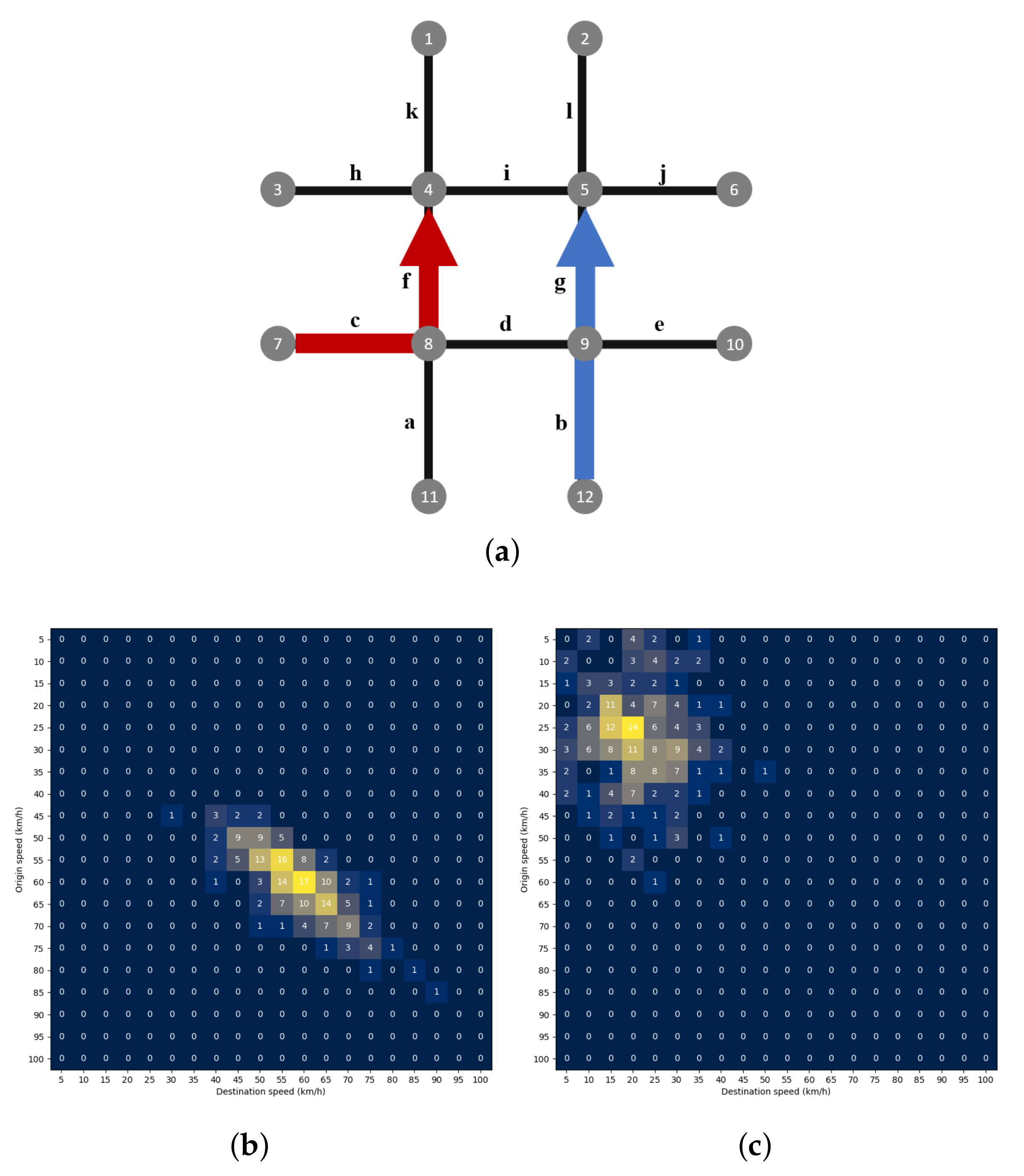
Most of the authors represent traffic data as a time series vector v R 1 × n [17] or a two-dimensional matrix M R m × n [22]. Dimensions m and n refer to the numbers of the road network segments (the spatial component) and the number of time intervals (the temporal component) of the observed road network. The STM concept is proposed on the Markov chain theory, where the transition matrix shows the probability of transition from one state to another. The STM is used to represent the probability of speed wchangehen traveling between two consecutive road network segments. In this paper, the road network is represented as a directed graph G = ( V , E ) , where V is a set of vertices representing intersections, and E is a set of edges representing road segments that connect two adjacent intersections. The transition is defined as a spatial change in vehicle trajectory when traveling from edge e i to edge e j in time interval t. As a traffic parameter under observation, the average speed is used. The average speed computed on e i labeled as the origin speed s o , and the average speed on the e j segment is labeled as destination speed s d . Two examples of the transition are visually represented in Figure 2a with red and blue colors. The transitions describe the vehicles traveling between edges c and f, and edges b and g. Subsequently, the STM matrix X is constructed as follows. First, all speed transitions from s o to s d between e i and e j are discretized and then counted within the particular time interval t. Each obtained value represent the count of transitions between s o and s d . The speed counts are further transformed into the speed transition probability distribution to obtain the probability for every transition. Values are put into the matrix X , which dimensions depend on the chosen resolution (sensitivity) of the speed change and the maximal observed speed. In this paper, 5 km/h is chosen as the speed discretization value and 100 km/h for the maximal possible speed, which resulted in matrix dimensions of 20 × 20 . The specific maximal speed value is chosen, because experiments are conducted on the road segments with a speed limit between 50 and 80 km/h. Equation (1) presents the STM, where every value p i j represents the probability that the vehicle had origin speed s o and destination speed s d in the observed transition at time interval t.
Figure 2b,c show two examples of the STM. Example (b) represents normal traffic flow as the high-speed values are present on both origin and destination segments, and (c) represents congested traffic flow, as speed is speed much lower when compared to the free flow speed. It can be noted that the position of the captured pattern is important information for the traffic state estimation.
X = p 11 p 12 p 1 n p 21 p m 1 p m n

3.2. Center of Mass Estimation

This method presents a simple but effective feature extraction process. The feature, in this case, is the position of the traffic pattern extracted from the STM. The COM’s position is the single most important information that is useful for the traffic state estimation problem when using the STMs, as the position can indicate different traffic conditions. If placed in the upper left corner, the position indicates that the average speed is very low if compared to the speed limit and traffic state can be declared as heavily congested. For the lower left corner, the position indicates very high speed on origin road segments while, at the same time, the speed is extremely low on the destination road segment. The same behavior can be noticed if COM is located in the upper right corner, where speed values are low on the origin, and extremely high on the destination road segment. If the COM coordinates are positioned in the center of the matrix or in the lower right corner, it indicates that the speed values on both origin and destination road segments are relatively close or higher than the speed limit. This behavior can be interpreted as normal traffic behavior, as the speed value points to traffic flow without congestion. If COM’s position is located in-between mentioned traffic states, the traffic state could be declared unstable.
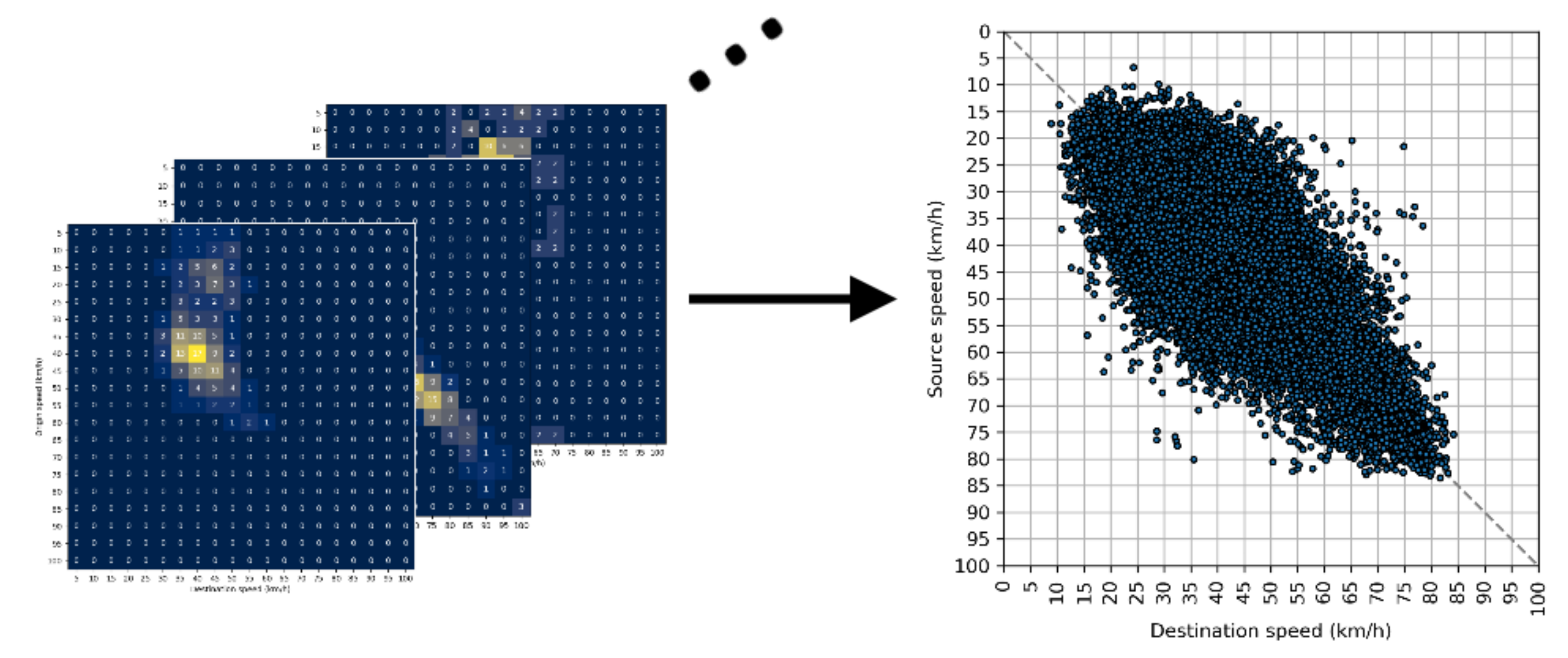
STMs are transformed to extract the COM in order to simplify the classification process. As the result, the 20 × 20 STM is represented by COM coordinates, c x , and c y . Subsequently, all of the points with coordinates c x and c y can be plotted in a two-dimensional space and clustered by the position in the coordinate system. Figure 3 represents the transformation from STMs and simplification to COMs plotted all in one coordinate system.
For the COM estimation, a method that is based on the computation of the expected coordinate values is used [31]. First, marginal distributions for the x and y coordinates are computed while using (2) and (3):
p x ( x j ) = i = 1 m p i j j = 1 , 2 , , n
p y ( y i ) = j = 1 n p i j i = 1 , 2 , , m
where p x is a marginal distribution of the x coordinates of the STM, and p y is a marginal distribution of the y coordinates of the STM. Afterwards, x and y coordinates of the COM are computed as the expected values:
c x = j = 1 n p x ( x j ) · j
c y = i = 1 m p y ( y i ) · i
where c x is a x coordinate of the COM, and c y is a y coordinate of the COM.

3.3. Clustering

In this paper, clustering aims to find groups of traffic patterns that are represented as STMs used to represent the current traffic state on the observed road segment. Three classes of traffic state were used, namely “Free flow”, “Stable flow”, and “Congestion”. This approach is used to characterize not only the congested traffic state but to describe all states that can occur on the traffic network. The “Free flow” class describes the traffic conditions when a vehicle travels on an empty road or with speed close to the speed limit. The "Stable flow” class describes traffic conditions that most drivers feel as “normal”, when drivers experience speed reductions, but the traffic is flowing smoothly most of the time. The “Congestion” class indicates traffic conditions with a strong decrease in travel speed and increased travel times on the traffic road network.

3.3.1. Agglomerative Clustering

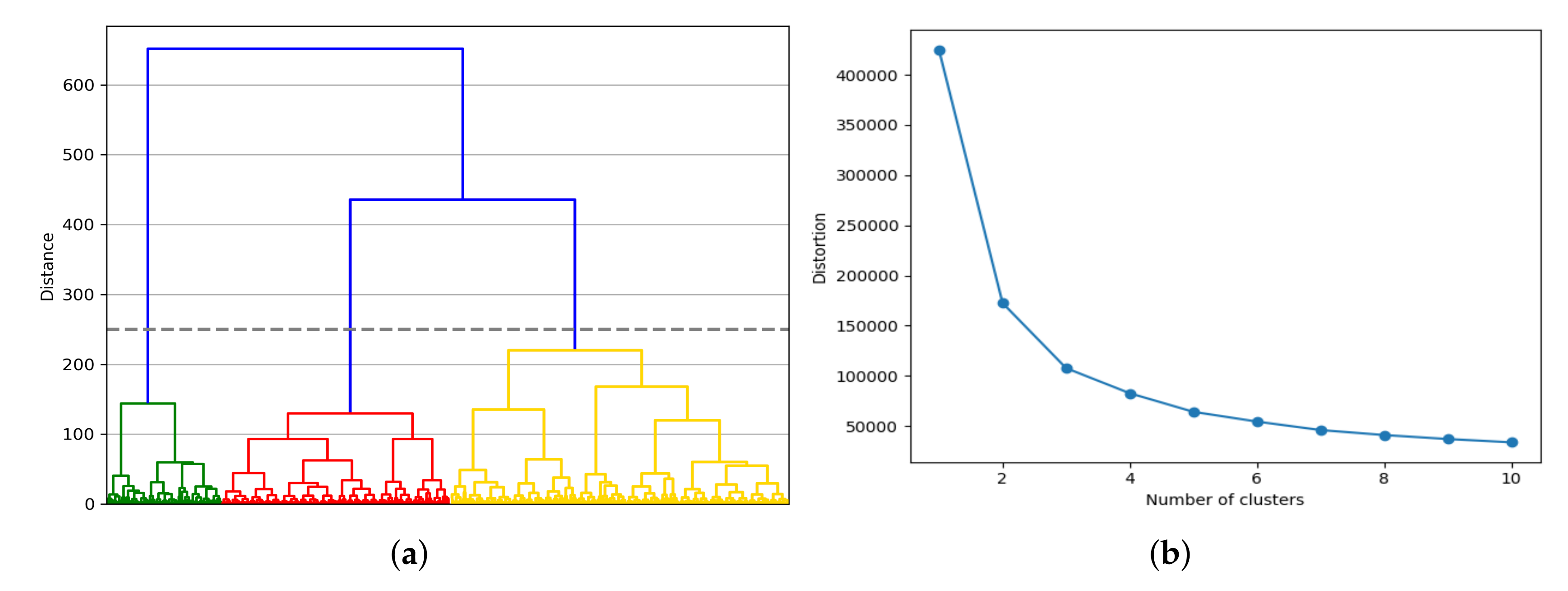
The hierarchical clustering is chosen for the clustering method. This approach constructs a hierarchical representation of a dataset, which presents an overview of the distribution of existing COMs extracted from STMs. This approach’s advantage is in providing the ability of reproducibility of resulting clusters and it provides more explanatory results [25]. There are two types of hierarchical clustering: (i) agglomerative and (ii) divisive. The approaches differ by way of constructing binary tree representation. The agglomerative approach uses a top-down, and the divisive approach uses the bottom-up strategy. In this paper, the agglomerative approach is used. It initiates each pattern as a single cluster and measures the distance between patterns and intermediate clusters. Subsequently, in every iteration, it combines the two closest patterns into a new cluster. The process is repeated until only one cluster remains. Figure 4a shows the results of an agglomerative clustering presented by dendrogram plot.

3.3.2. Clustering Validation

The elbow curve is presented for the observed data in order to confirm the number of clusters. In the cluster analysis process, the elbow curve is a heuristic used to determine the number of clusters in the dataset. Figure 4b presents the elbow curve with distortion plotted against the different number of clusters. The “elbow” can be detected in the part of the curve where the number of clusters is 3. At this point, the further increase of the number of clusters would not significantly contribute to the clustering quality. This value is used for the number of clusters for further experiments.
As the first validation technique of the classification process, cross-validation is adopted from [29,32]. For the cross-validation process, the 1000 data instances (COMs) from every class are randomly selected and labeled based on the visual inspection. The selected dataset is then separated into the training and test sets with a ratio of 80% for training and 20% for testing. The labeled dataset is then used as a ground truth value and compared to the agglomerative clustering results.
The second validation process is related to comparing the resulting classes with the domain knowledge data. The well-known HCM values of the Level of Service (LoS) are used to represent the specific domain knowledge data for the traffic state estimation process. HCM defines six levels of service for road segments that are based on driving speed values, from A to F, with LoS A representing the best driving conditions and LoS F the worst. Label A represents the best traffic conditions, with vehicle speeds larger than 80% of the free-flow speed, while label F represents the most extreme congestion, where vehicle speeds are less than 30% of the free-flow speed [33]. LoS quantifies the increase in travel time due to the conditions on the road segments and it is also a measure of driver discomfort, and fuel consumption. In this paper, LoS values are used to validate the traffic state estimation process. Firstly, the LoS values are merged in three classes in following way: (i) free-flow traffic conditions represented by the LoS labeled as A and B, (ii) traffic conditions represented by the LoS labeled with C and D are labeled as stable, and (iii) congested traffic conditions that are represented with LoS are labeled with E and F. Then, the same test dataset for the cross-validation is labeled with three classes. The labeled dataset is then used as a ground truth value and compared to the agglomerative clustering results.

4. Results

4.1. Data

The large real-life FCD acquired from the vehicles equipped with the tracking devices is used. Each record contains a time-stamp, geographical longitude and latitude, speed, and heading. Due to the storage limitation, most of the data are sampled in the following way: 100 m for vehicles in driving mode and every 5 min. for turned off vehicles. Raw data are map matched to the road segments in a digital map based on the measured latitude, longitude, and heading. Data that could not be matched to appropriate road-segment due to the errors caused by tunnels, high building concentration, or other causes were filtered out. GNSS data for Croatia’s road network were recorded for five years between August 2009 and October 2014 by approximately 4200 tracked vehicles. The tracked vehicle fleet is versatile and mostly consists of delivery vehicles (vans, caddies, small trucks) and taxi cars. The historically tracked data, which consist of 6 , 55 billion records, was provided by Mireo Inc. as a part of the SORDITO project [34]. In this paper, we analyze the data and estimate traffic state using the proposed method for some of the most relevant road segments and intersections in the City of Zagreb, the capital, and the largest city in Croatia.
The seasonality of the traffic flow is considered in order to lower the deviation. Summer months, July and August, are excluded from the experiment. They significantly influence the results on the road network of Zagreb, due to the different, and lower traffic flows that are caused by vacations [35]. Data are further divided into two groups: working days and weekend days. Working day data, Monday to Friday, show different traffic conditions when compared to the weekend data (Saturday and Sunday), mostly due to the daily commuters and, therefore, the weekend data are also excluded.

4.2. Traffic State Estimation

Results of a traffic state estimation are shown for the eight time intervals throughout a day. Time intervals are defined by [34,36] for the congestion estimation problem based on the same real-life FCD dataset that refers to speed data for the City of Zagreb. Intervals are defined, as follows: (i) 05:30–06:45 as morning interval with very small traffic volume, (ii) 06:45–07:25 as interval before the morning rush hour, (iii) 07:25–08:20 as morning rush hour, (iv) 08:20–15:30 as interval between morning and evening rush hour, (v) 15:30–17:05 as evening rush hour, (vi) 17:05–19:00 as interval after evening rush hour, (vii) 19:00–22:00 as interval that represent evening traffic conditions, and (viii) 22:00–05:30 as the night interval.
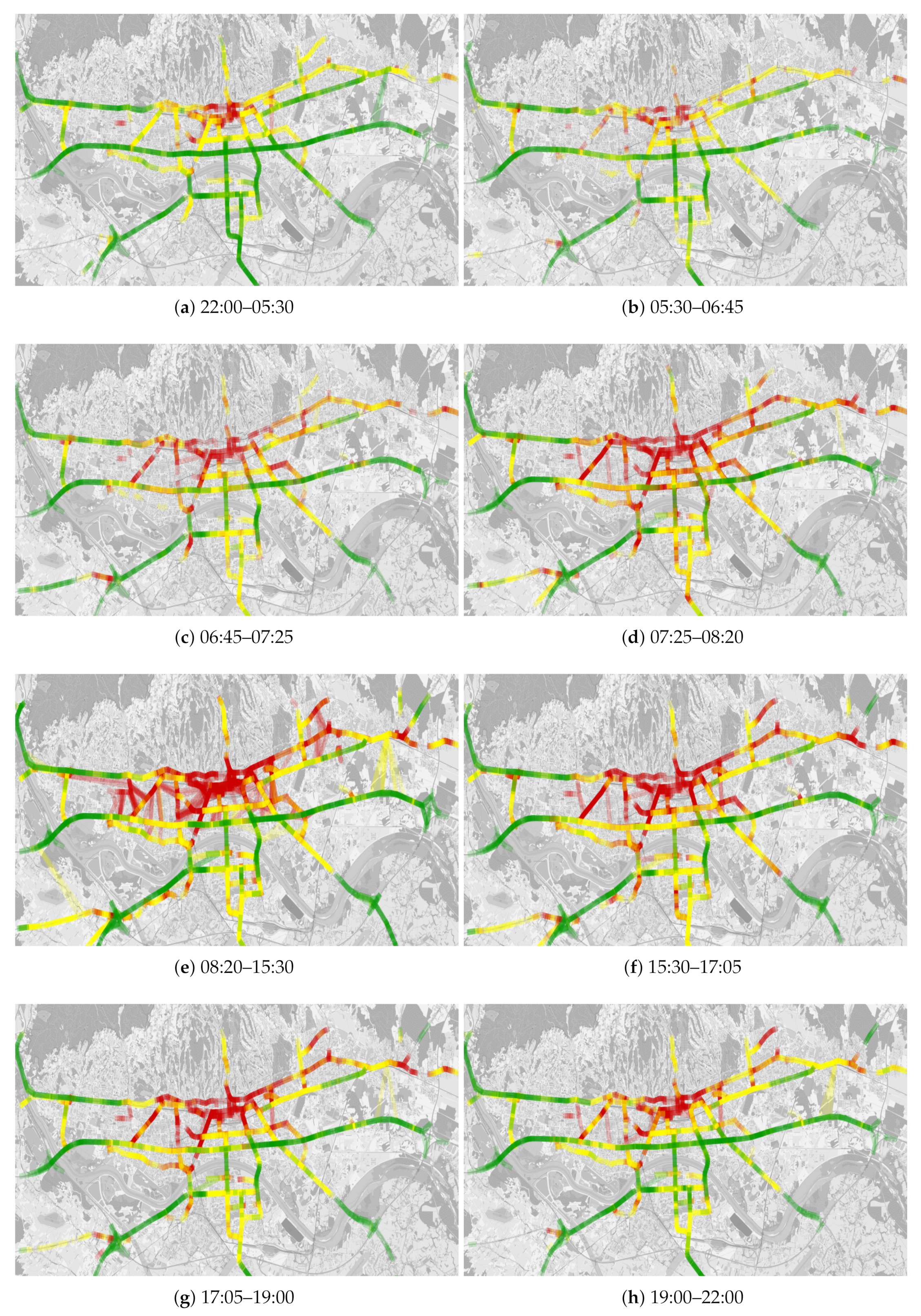
Table 1 represents the results for the traffic state estimation grouped into three classes. The results are shown while using the ratios between the number of classified transitions and the total number of transitions in the observed time interval. The rows show the distribution of classified transitions in the observed time interval. Rush hours are highlighted and, as expected, have the largest values of the transitions labeled as congested. The time interval between rush hours shows the largest value of the ratio for the congested transitions. This indicates that congestion that started in the morning rush hour is prolonged to the next time interval. This also could indicate that congestion starts at the interval between rush hours and is prolonged to the evening rush hour. This kind of behavior could indicate inefficient traffic regulations on observed transitions. The ratio of the congested roads in the time interval of 17:05–19:00, shows a large portion of the transitions classified as congested, although it is not the rush hour interval. This behavior can be addressed to the city attractions placed in the city center and people visiting such locations in their free time. This fact can be confirmed by the classes’ spatial distribution that is presented in Figure 5g.
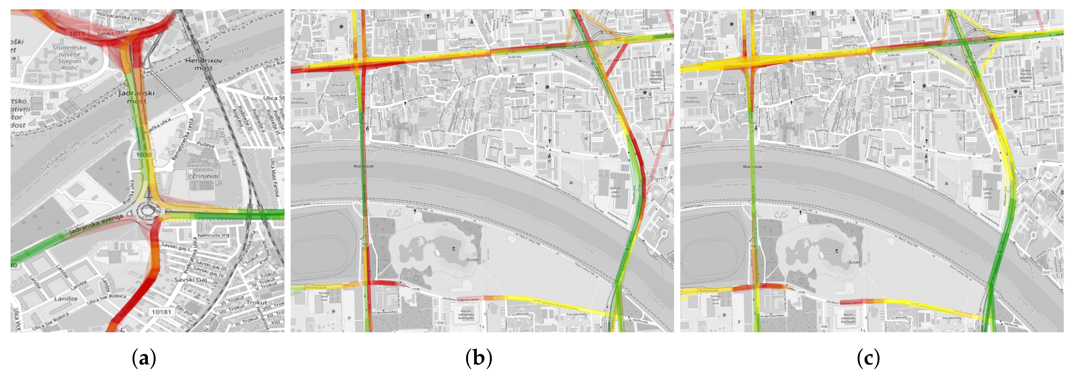
Figure 5 shows the spatial distribution of the classified traffic patterns for every observed time interval. The colors used for the visualizations are: (i) red—“Congestion”, (ii) yellow—“Stable flow”, and (iii) green—“Free flow”. It can be noticed that the congestion level is the highest in the city center and the west part of the city. Some congestion patterns can be extracted by analyzing all time intervals. For example, the southern part of the city represents the business area. The congestion appears only in the morning and evening rush hours due to the daily commuters. Visualization of the congestion patterns can be used for more in-depth and more granular analysis of the traffic state. For the case study, Zagreb’s three most important bridges across Sava river are chosen, which divide the southern and north part of the city. The bridge Jadranski most is detected as the most congested bridge. Figure 6a shows the enlarged image of the traffic congestion estimation results for the Jadranski most in the rush hours. The results show the most congested approaches to the bridge and the roundabout at the southern approach. The figure shows that STMs can estimate traffic state at micro-locations and consider the direction of the traffic flow. It can be observed that direction from south to north is more congested than the opposite one. The same behavior can be noticed in the afternoon rush hour.
On the other hand, different behavior can be observed on the other two bridges, namely Most slobode (left) and Most mladosti (right), as shown in Figure 6b,c. The traffic state estimation results show different behavior in the morning and afternoon peak hours. In the morning peak hours, the traffic congestion is increased in a direction towards the city (south to north), which indicates the increase in traffic demand due to the commuters, while the other direction (north to south) represents the normal or free-flow conditions. In the afternoon peak hours, both bridges’ flow indicates the normal or free-flow conditions, and congestion occurs at the intersections due to inadequate traffic lights signalization.

4.3. Validation Results

The results for both validation processes are reported while using the confusion matrices and the classification report that shows the total accuracy of the model, precision, recall, and F1 scores for every class. The confusion matrix reports the performance of the classification in a visual manner. Each row of the matrix represents the ground truth values, while the columns present the predicted class labels. The values in the matrix represent the accuracy of the prediction computed as a number of data instances that are correctly classified divided by all of the data provided for the considered class.
In classification problems with more than two classes, the precision is computed as the sum of the true positive values, divided by the sum of true positive and false positive values computed across all classes. The F1 scores are computed as the harmonic mean of precision and recall. The accuracy is the measure for the accuracy of the model computed across all classes by averaging the total true positive, false negative, and false positive values.
Table 2 presents the classification report for the cross-validation method. The validation achieved the average prediction accuracy of 97%. The recall of the class labeled as “Free flow” with a value 84% shows that, even the precision shows the perfect score, there are some values that are not classified correctly. If Table 3 (confusion matrix) is observed, it can be seen that 15.9% of the values of the class “Free flow” are labeled as “Stable flow”. The results of the cross-validation method indicate that the classes labeled with “Stable flow” and “Congestion” are well separated and they can be classified with high accuracy, while classes that are labeled as “Free flow” and “Stable flow” to some extent are harder to separate.
Table 4 presents the classification report for the validation that is based on the domain knowledge extracted from the HCM. The validation achieved the average prediction accuracy of 91%. The lower prediction accuracy can be accounted to the strict boundaries of defined LoS values. The lowest precision value can be noticed in the class labeled as unstable operations. If the corresponding confusion matrix is observed in Table 5, it can be seen that 19.1% of unstable traffic instances are predicted as congested traffic and 4.6% are predicted as normal traffic.

5. Discussion

In this paper, novel traffic data representation in the form of the STM is proposed. This section describes the potential application of the STM in traffic-related research and applications, and highlights some drawbacks that need to be addressed in further research. This section also emphasizes expected impact for academia, such as using STMs for visualization, quantifying, and classifying traffic state, capturing the changes in the speeds on a road network, identifying the anomalous behavior, and using COM’s movement for presenting the probability of traffic state change or the capturing complex traffic patterns that can be used to identify potentially dangerous traffic situations.
Alongside the presented application of the method, it has some drawbacks that need to be addressed. Traffic state value is only based on the speed values. This could be a problem on short road segments bounded by unsynchronised traffic lights because vehicles would have very low speeds due to the traffic light’s signal plan. Regarding this property, the traffic state could be wrongly estimated as very high. Secondly, sparse GNSS data is used, which entails wide time intervals for the experiment. Commonly used, shorter time intervals like 5-, 15-, 30-, or 60-min could give better insight on the traffic state and, thus, on the traffic state on the observed road segments. In this paper, the dataset used for the experiment is data that only include working days to only capture the most extreme congestion conditions in the urban road network. A possible improvement would be to include the weekend data to analyze the differences between traffic in working and weekend traffic flow fluctuations.

5.1. Traffic State Estimation

In this paper, the use of the STM is proposed to estimate and classify the traffic state on the urban road network. It is shown that the STM can be useful for the visualization, quantifying, and classifying traffic state. The STM is a possible traffic data modeling approach for traffic state prediction. The proposed data model can be used as a set of images for training some machine learning model in order to predict the future state of traffic. The full potential of the STMs can be utilized in (near) real-time analysis when the position of the COM for every STM is changing over the observed time period. The position itself and the movement of the COM (positions in the past observed intervals) could provide usable and actionable information for traffic management systems. The COM’s movement indicates the change in traffic state and can present the probability of traffic state change, which is an important factor in the traffic state prediction problem.

5.2. Routing Applications

The routing applications benefit the most from the traffic state estimation and prediction. Every route planner must include current, and possibly future, traffic state information to enable fast and secure delivery. Traffic state estimation based on the STM can provide useful information regarding the congestion, and therefore routing through the less congested roads. The framework for solving the well-known routing problem Time-Dependent Vehicle Routing Problem, is presented in [36]. The authors used speed profiles to extract the congestion zones and quantified the congestion by computing the slowdown coefficients using the travel times. The STM can be used in both steps. The congestion zones can be identified based on the position of the COM, while the same point represents the slowdown probability on the observed road segments.

5.3. Anomaly Detection

Anomaly detection is a crucial part of ITS, especially in the incident management domain. The detection of the recurrent anomalies like heavy congestion could improve reaction time and give some actionable information for the traffic management authorities. On the other side, fast detection of non-recurrent anomalies, like traffic incidents, could even save a human life. STM presents an opportunity to capture the changes in the speeds on the observed road network, and identify the potential anomalous behavior. In contrast to the speed profiles, the STM provides a two-dimensional distribution of speed on consecutive road segments in an observed time interval. It enables the capture of a more complex traffic patterns that can be used to identify potentially dangerous traffic situations. As one of the applications for anomaly detection, traffic bottleneck detection and propagation can be represented while using STMs. The STM presents the tool to capture, visualize, and analyze the bottlenecks’ impacts on the road network. The bottlenecks result in traffic congestion on one part of the network caused by the traffic accident, badly timed traffic lights, or slow vehicles that disrupt the traffic flow. The STM can capture such scenarios. The COM’s position in the upper right corner, or in the lower-left corner, could indicate a serious accident, as it shows very high-speed values on one road segment if compared to its consecutive one with very low-speed values.

6. Conclusions and Further Research

This paper presents a novel traffic data representation of the GNSS dataset by using the STMs. The methodology is presented for the traffic state estimation and classification on a citywide scale. The COM for every matrix was extracted to classify the STMs. This approach resulted in simplification of the classification process and higher interpretability of the resulting classes. The results show that STMs can be used to estimate the traffic state on a citywide scale and on micro-locations. The results are validated using the cross-validation method, and specific domain knowledge, which resulted in an accuracy of 97% and 91%, respectively.
As presented in the discussion section, the STM is a traffic data representation model that shows multiple possible implementation possibilities in different traffic and transport-related research and applications. Some of the applications are: (i) real-time traffic state estimation, (ii) routing applications, and (iii) anomaly detection in traffic data by identifying unusual traffic patternsthat are captured by the STM.
There are multiple possible further research directions for the academic community. The first one could include training a deep learning model that is based on the Convolutional Neural Network (CNN) as a traffic state classifier. The STM is a data model that formed as a traffic image that can be used as input data for training the CNN. The second one would include a tensor-based analysis. Traffic tensor could be created as multiple STMs placed in the tensor-based on the time interval, in which the STM is collected. Subsequently, a tensor-based analysis could give more spatiotemporal insight into traffic conditions.

Author Contributions

Conceptualization, L.T. and T.C.; Methodology, L.T.; Software, L.T.; Validation, L.T.; Formal analysis, L.T.; Resources, T.C.; Writing–original draft preparation, L.T.; Writing–review and editing, L.T., T.C., T.F., B.A.; Visualization, L.T.; Supervision, T.C., T.F., B.A.; Funding acquisition, T.C. All authors have read and agreed to the published version of the manuscript.

Funding

This research has been supported by the European Regional Development Fund under the grant KK.01.1.1.01.0009 (DATACROSS). This research is partially supported by Croatian Science Foundation under project IP-2018-01-8323. Data used for this research is collected during project SORDITO, European Regional Development Fund under contract RC.2.2.08-0022.

Acknowledgments

Authors are very grateful to industrial partner MIREO Inc. and the Faculty of Transport and Traffic Sciences, University of Zagreb for their contribution.

Conflicts of Interest

The authors declare no conflict of interest.

References

  1. Gregurić, M.; Mandžuka, S.; Vidović, K. Advanced Applications for Urban Motorway Traffic Control. In Lecture Notes in Networks and Systems; Springer: Berlin/Heidelberg, Germany, 2020; Volume 76, pp. 395–400. [Google Scholar] [CrossRef]
  2. European Commission. Sustainable Urban Mobility: European Policy, Practice and Solutions. Available online: https://ec.europa.eu/transport/sites/transport/files/2017-sustainable-urban-mobility-european-policy-practice-and-solutions.pdf (accessed on 14 July 2020).
  3. Chow, A.H.; Santacreu, A.; Tsapakis, I.; Tanasaranond, G.; Cheng, T. Empirical assessment of urban traffic congestion. J. Adv. Transp. 2014, 48, 1000–1016. [Google Scholar] [CrossRef] [Green Version]
  4. Cambridge Systematics. Traffic Congestion and Reliability: Trends and Advanced Strategies for Congestion Mitigationt (Tech Report). Available online: https://rosap.ntl.bts.gov/view/dot/20656 (accessed on 15 July 2020).
  5. Servos, N.; Liu, X.; Teucke, M.; Freitag, M. Travel Time Prediction in a Multimodal Freight Transport Relation Using Machine Learning Algorithms. Logistics 2019, 4, 1. [Google Scholar] [CrossRef] [Green Version]
  6. Pun-Cheng, L.S.C. An Interactive Web-Based Public Transport Enquiry System With Real-Time Optimal Route Computation. IEEE Trans. Intell. Transp. Syst. 2012, 13, 983–988. [Google Scholar] [CrossRef]
  7. Ouyang, Q.; Lv, Y.; Ma, J.; Li, J. An LSTM-Based Method Considering History and Real-Time Data for Passenger Flow Prediction. Appl. Sci. 2020, 10, 3788. [Google Scholar] [CrossRef]
  8. Mandžuka, S.; Ivanjko, E.; Vujić, M.; Škorput, P.; Gregurić, M. The Use of Cooperative ITS in Urban Traffic Management. In Intelligent Transport Systems: Technologies and Applications; Wiley: Chichester, UK, 2016; pp. 361–381. [Google Scholar]
  9. Škrinjar, J.; Abramović, B.; Bukvić, L.; Marušić, Z. Managing Fuel Consumption and Emissions in the Renewed Fleet of a Transport Company. Sustainability 2020, 12, 5047. [Google Scholar] [CrossRef]
  10. Herrera, J.C.; Work, D.B.; Herring, R.; Ban, X.J.; Jacobson, Q.; Bayen, A.M. Evaluation of traffic data obtained via GPS-enabled mobile phones: The Mobile Century field experiment. Transp. Res. Part Emerg. Technol. 2010, 18, 568–583. [Google Scholar] [CrossRef] [Green Version]
  11. Herrera, J.C.; Bayen, A.M. Incorporation of Lagrangian measurements in freeway traffic state estimation. Transp. Res. Part B Methodol. 2010, 44, 460–481. [Google Scholar] [CrossRef]
  12. Kong, Q.; Zhao, Q.; Wei, C.; Liu, Y. Efficient Traffic State Estimation for Large-Scale Urban Road Networks. IEEE Trans. Intell. Transp. Syst. 2013, 14, 398–407. [Google Scholar] [CrossRef]
  13. Erdelić, M.; Carić, T.; Ivanjko, E.; Jelušić, N. Classification of travel modes using streaming GNSS data. In Transportation Research Procedia; Elsevier B.V.: Amsterdam, The Netherlands, 2019; Volume 40, pp. 209–216. [Google Scholar] [CrossRef]
  14. Rakha, H.; Tawfik, A. Traffic Networks: Dynamic Traffic Routing, Assignment, and Assessment. In Encyclopedia of Complexity and Systems Science; Meyers, R.A., Ed.; Springer: New York, NY, USA, 2009; pp. 9429–9470. [Google Scholar] [CrossRef]
  15. Wahle, J.; Annen, O.; Schuster, C.; Neubert, L.; Schreckenberg, M. A dynamic route guidance system based on real traffic data. Eur. J. Oper. Res. 2001, 131, 302–308. [Google Scholar] [CrossRef]
  16. Juhász, J. Influence of Different Route-choice Decision Modes. Transp. Res. Procedia 2017, 27, 246–252. [Google Scholar] [CrossRef]
  17. Erdelić, T.; Ravlić, M.; Carić, T. Travel time prediction using speed profiles for road network of Croatia. In Proceedings of the 2016 International Symposium ELMAR, Zadar, Croatia, 12–14 September 2016; pp. 97–100. [Google Scholar] [CrossRef]
  18. Ma, X.; Dai, Z.; He, Z.; Ma, J.; Wang, Y.; Wang, Y. Learning traffic as images: A deep convolutional neural network for large-scale transportation network speed prediction. Sensors 2017, 17, 818. [Google Scholar] [CrossRef] [PubMed] [Green Version]
  19. Nguyen, H.; Liu, W.; Chen, F. Discovering Congestion Propagation Patterns in Spatio-Temporal Traffic Data. IEEE Trans. Big Data 2017, 3, 169–180. [Google Scholar] [CrossRef]
  20. Afrin, T.; Yodo, N. A Survey of Road Traffic Congestion Measures towards a Sustainable and Resilient Transportation System. Sustainability 2020, 12, 4660. [Google Scholar] [CrossRef]
  21. Rao, M.; Rao, K.R. Measuring Urban Traffic Congestion—A Review. Int. J. Traffic Transp. Eng. 2012, 2, 286–305. [Google Scholar] [CrossRef] [Green Version]
  22. Liu, X.; Liu, X.; Wang, Y.; Pu, J.; Zhang, X. Detecting Anomaly in Traffic Flow from Road Similarity Analysis. In Web-Age Information Management; Cui, B., Zhang, N., Xu, J., Lian, X., Liu, D., Eds.; Springer International Publishing: Cham, Switzerland, 2016; pp. 92–104. [Google Scholar] [CrossRef] [Green Version]
  23. Kerner, B. Empirical macroscopic features of spatial-temporal traffic patterns at highway bottlenecks. Phys. Rev. E Stat. Nonlinear Soft Matter Phys. 2002, 65, 046138. [Google Scholar] [CrossRef]
  24. Kerner, B.S.; Rehborn, H.; Aleksic, M.; Haug, A. Recognition and tracking of spatial–temporal congested traffic patterns on freeways. Transp. Res. Part C Emerg. Technol. 2004, 12, 369–400. [Google Scholar] [CrossRef]
  25. Nguyen, T.T.; Krishnakumari, P.; Calvert, S.C.; Vu, H.L.; van Lint, H. Feature extraction and clustering analysis of highway congestion. Transp. Res. Part C Emerg. Technol. 2019, 100, 238–258. [Google Scholar] [CrossRef]
  26. Kim, J.; Mahmassani, H.S. Spatial and temporal characterization of travel patterns in a traffic network using vehicle trajectories. Transp. Res. Part C Emerg. Technol. 2015, 59, 375–390. [Google Scholar] [CrossRef]
  27. Thianniwet, T.; Phosaard, S.; Pattara-Atikom, W. Classification of Road Traffic Congestion Levels from GPS Data using a Decision Tree Algorithm and Sliding Windows. In Proceedings of the World Congress on Engineering (WCE), London, UK, 1–3 July 2009; pp. 1–5. [Google Scholar]
  28. Jin, X.; Srinivasan, D.; Cheu, R.L. Classification of freeway traffic patterns for incident detection using constructive probabilistic neural networks. IEEE Trans. Neural Netw. 2001, 12, 1173–1187. [Google Scholar] [CrossRef]
  29. Kan, Z.; Tang, L.; Kwan, M.P.; Ren, C.; Liu, D.; Li, Q. Traffic congestion analysis at the turn level using Taxis’ GPS trajectory data. Comput. Environ. Urban Syst. 2019, 74, 229–243. [Google Scholar] [CrossRef]
  30. Keler, A.; Ding, L.; Krisp, J. Visualization of traffic congestion based on Floating Taxi Data. Kartographische Nachrichten 2016, 66, 7–13. [Google Scholar] [CrossRef]
  31. Jordaan, I.J. Decisions under Uncertainty: Probabilistic Analysis for Engineering Decisions; Cambridge University Press: Cambridge, UK, 2005; pp. 127–144. [Google Scholar] [CrossRef]
  32. Nguyen, H.N.; Krishnakumari, P.; Vu, H.L.; van Lint, H. Traffic Congestion pattern classification using multi-class SVM. In Proceedings of the 2016 IEEE 19th International Conference on Intelligent Transportation Systems (ITSC), Rio de Janeiro, Brazil, 1–4 November 2016; pp. 1059–1064. [Google Scholar] [CrossRef]
  33. HCM2010. Highway Capacity Manual; Transportation Research Board, National Research Council: Washington, DC, USA, 2010. [Google Scholar]
  34. Carić, T.; Erdelić, T.; Fosin, J.; Matulin, M.; Erdelić, M.; Rožić, L.; Milošević, A. Technical Report of Project SORDITO; Technical Report; Faculty of Transport and Traffic Sciences: Zagreb, Croatia, 2016. [Google Scholar]
  35. Żochowska, R.; Karoń, G. ITS Services Packages as a Tool for Managing Traffic Congestion in Cities. In Intelligent Transportation Systems—Problems and Perspectives; Sładkowski, A., Pamuła, W., Eds.; Springer International Publishing: Cham, Switzerland, 2016; pp. 81–103. [Google Scholar] [CrossRef]
  36. Carić, T.; Fosin, J. Using Congestion Zones for Solving the Time Dependent Vehicle Routing Problem. Promet-Traffic Transp. 2020, 32, 25–38. [Google Scholar] [CrossRef]
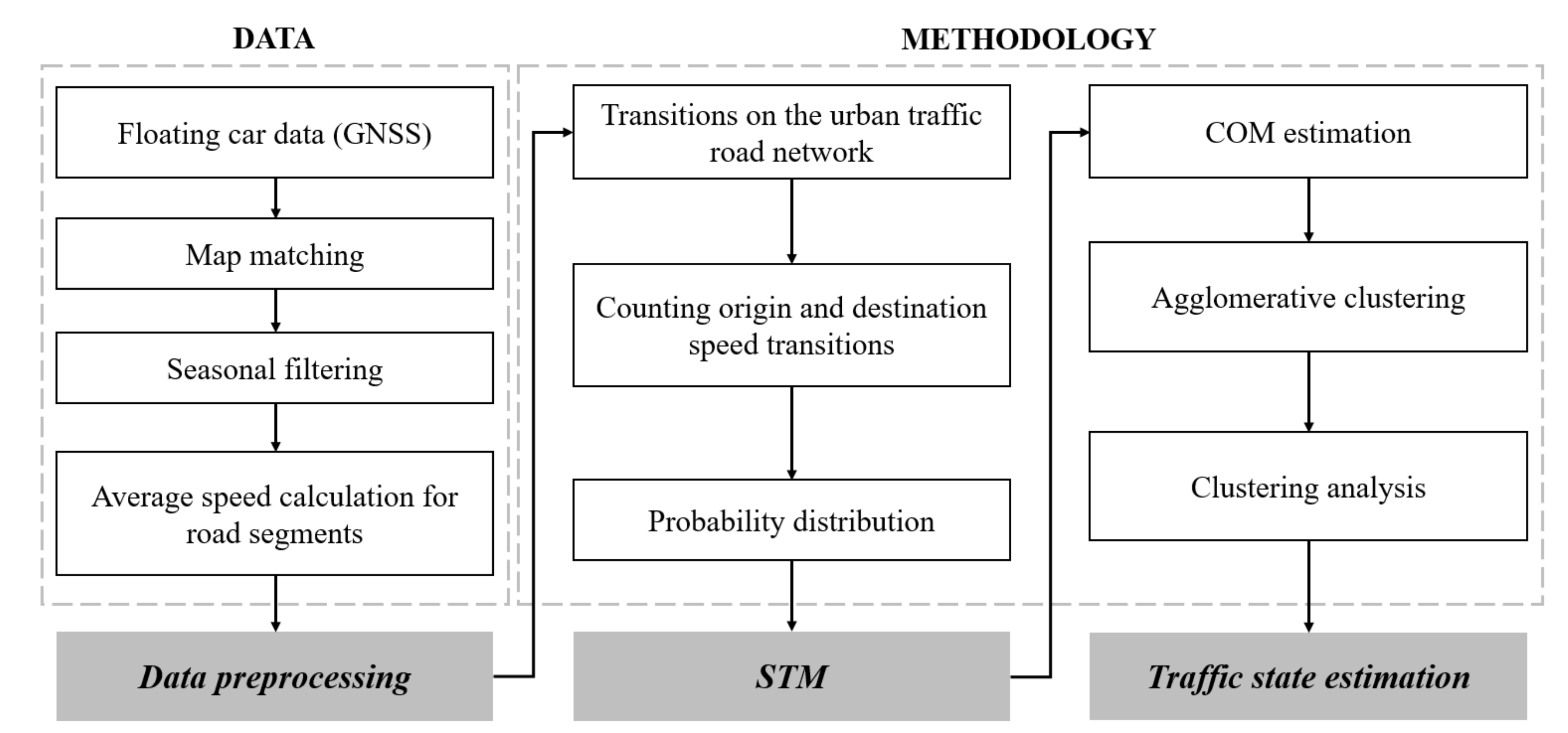
Figure 1. The methodology for the traffic state estimation and classification based on the Center Of Mass (COM) estimation of the speed data represented using Speed Transition Matrices (STMs).
Sustainability 12 07278 g001
Figure 2. (a) Example of transitions on a simple road network, (b) STM representing the normal traffic flow, and (c) STM representing the congestion.
Sustainability 12 07278 g002
Figure 3. Representing the three dimensional STM data with the two dimensional COM coordinates.
Sustainability 12 07278 g003
Figure 4. (a) Result of the agglomerative clustering approach, and (b) the elbow method results.
Sustainability 12 07278 g004
Figure 5. Results of traffic state estimation visualized on the map of the City of Zagreb.
Sustainability 12 07278 g005
Figure 6. (a) Traffic state on the Jadranski most in both peak hours, (b) Traffic state on the bridges Most slobode and Most mladosti in the morning peak hours, and (c) Traffic state on bridges Most slobode and Most mladosti in the afternoon peak hours.
Sustainability 12 07278 g006
Table 1. Results of traffic state estimation represented using three classes.
Free FlowStable FlowCongestion
22:00–05:3028.31%54.15%17.54%
05:30–06:4527.38%53.55%19.08%
06:45–07:2519.08%42.83%38.10%
07:25–08:2013.97%32.53%53.50%
08:20–15:3012.09%33.86%54.05%
15:30–17:0513.05%35.46%51.04%
17:05–19:0015.53%40.59%43.88%
19:00–22:0019.77%46.33%33.90%
Table 2. Results of the cross validation.
PrecisionRecallF1 Score
Free flow1.000.840.91
Stable flow0.931.000.97
Congestion1.001.001.00
Accuracy 0.97
Table 3. Confusion matrix of the cross validation.
PredictedFree FlowStable FlowCongestion
Known
Free flow0.8410.1590
Stable flow01.0000
Congestion00.0030.997
Table 4. Results of validation using domain knowledge data.
PrecisionRecallF1 Score
Free flow0.990.950.97
Stable flow0.831.000.90
Congestion1.000.810.89
Accuracy 0.91
Table 5. Confusion matrix of validation using domain knowledge data.
PredictedFree FlowStable FlowCongestion
Known
Free flow0.9540.0460
Stable flow0.0040.9960
Congestion00.1910.809